Deep Filtering Thanks: This research was supported in part by the Army Research Office under grant W911NF-19-1-0176.
Abstract
This paper develops a deep learning method for linear and nonlinear filtering. The idea is to start with a nominal dynamic model and generate Monte Carlo sample paths. Then these samples are used to train a deep neutral network. A least square error is used as a loss function for network training. Then the resulting weights are applied to Monte Carlo samples from an actual dynamic model. The deep filter obtained in such a way compares favorably to the traditional Kalman filter in linear cases and the extended Kalman filter in nonlinear cases. Moreover, a switching model with jumps is studied to show the adaptiveness and power of our deep filtering method. A main advantage of deep filtering is its robustness when the nominal model and actual model differ. Another advantage of deep filtering is that real data can be used directly to train the deep neutral network. Therefore, one does not need to calibrate the model.
Keywords and Phrases: Deep neutral network, filtering, regime switching model.
1 Introduction
This paper develops deep learning methods for both linear and nonlinear filtering problems. Recent advent of applications of artificial intelligence in diversified domains has promoted an intensified interest in using machine learning theory to treat stochastic dynamic systems and stochastic controls. It opens up many possibilities in state estimation with reduced computational complexity, alleviating the curse of dimensionality. There are numerous successful applications of deep learning in multi-agent systems, traffic control, robotics, personalized recommendations, and games of GO and Atari. Despite many progresses, there seems to be no work devoted to using the deep learning approach in state estimation and filtering. This paper aims to develop deep neutral network based filtering schemes.
Deep Neutral Networks (DNN) and Backpropagation. Neural networks (NN) are often used to approximate functions, which are often complex and highly nonlinear, arising from a wide variety of applications. The main approaches are of compositional nature and rely on composition of hidden layers of base functions. A deep neural network is in fact, an NN with several hidden layers. The deepness of the network is measured by the number of layers used. In this paper, we only consider a fully connected NN and there are no connections between nodes in the same layer. A typical DNN diagram of such a class is depicted in Figure 1. For related literature on DNN, we refer the reader to the online book by Nielsen [10].

The backpropagation is a commonly used main driver in DNN training. By and large, backpropagation is an algorithm for supervised learning of artificial neural networks using gradient descent procedures. Given an artificial NN and a loss or error function, the scheme calculates the gradient of the loss function with respect to the weights of the neural network. The calculation of the gradient proceeds backwards through the network starting with the gradient of the final layer of weights. To facilitate the computation, partial computations of the gradient from one layer are reused for the previous layer’s gradient calculation. Such backwards flow of information is designed for efficient computation of the gradient at each layer. In particular, backpropagation requires three items:
- (a)
A data set consisting of fixed pairs of input and output variables;
- (b)
A feedforward NN with parameters given by the weights ;
- (c)
A loss (error) function defining the error between the desired output and the calculated output.
In this paper, the NN training will use the stochastic gradient decent method to find the weight vector to minimize a loss function . The details are to be given later.
Linear and Nonlinear Filtering. As is well known, filtering is concerned with dynamic systems in which the internal state variables are not completely observable. There are numerous real-world applications involving state estimation and filtering, including maneuvered target tracking, speech recognition, telecommunications, financial engineering, among many others. Traditional approaches derive estimators based on observations with least square errors. Working at a setup in discrete time for the underlying systems and under a Gaussian distribution framework, the corresponding filtering problem is to find the conditional mean of the state given the observation up to time . The best known filter is the Kalman filter for linear models. As for some nonlinear models, extended Kalman filters can be applied. We refer the reader to Anderson and Moore [1] for more details.
Early development in nonlinear filtering can be found in Duncan [3], which focuses on conditional densities for diffusion processes, Mortensen [9], which concentrates on the most probable trajectory approach; Kushner [11], which derives nonlinear filtering equations, and Zakai [14], which uses unnormalized equations.
There are many progresses made in the past decades since then. For example, hybrid filtering can be found in Hijab [7] with an unknown constant, Zhang [15] with small observation noise, Miller and Runggaldier [8] with Markovian jump times, Blom and Bar-Shalom [2] for discrete-time hybrid model and the Interactive Multiple Model algorithm, Dufour et al [4, 5] and Dufour and Elliott [6] for models with regime switching. Some later developments along this line can be found in Zhang [15, 16, 17]. Despite these important progresses, the computation of filtering remains a daunting task. For nonlinear filtering, there have been yet feasible and efficient schemes to mitigate high computational complexity (with infinite dimensionality). Much effort has been devoted to finding computable approximation schemes.
Deep Filtering. In this paper, we propose a new framework, which focuses on deep neutral network based filtering. Under a given model, the idea is to generate Monte Carlo samples and then use these samples to train a deep neutral network. The observation process generates inputs to the DNN; the state from the Monte Carlo samples is used as the target. A least square error of the target and calculated output is used as a loss function for network training for weight vectors. Then these weight vectors are applied to another set of Monte Carlo samples of the actual dynamic model. The corresponding calculated DNN output is termed a deep filter (DF).
In this paper, we demonstrate the adaptiveness, robustness, and effectiveness of our DF through numerical examples. The deep filter compares favorably to the traditional Kalman filter in linear cases and the extended Kalman filter in nonlinear cases. Moreover, a switching model with jumps is studied and used to show the feasibility and flexibility of our deep filtering. A major advantage of deep filter is its robustness when the nominal model and actual model differ. Another advantage of the deep filtering is that real data can be used directly to train the deep neutral network. Therefore, model calibration is no longer needed in applications.
The rest of the paper is arranged as follows. Section 2 begins with our deep filtering algorithm, followed by its corresponding versions for linear models, nonlinear models, and switching models. Numerical experiments are presented. Performance of the deep filter is examined through various models and compared with benchmark linear and nonlinear filters. Concluding remarks are provided in Section 3.
2 Deep Filter
Let denote the state process with system equation
for some suitable functions and system noise with . A function of can be observed with possible noise corruption. In particular, the observation process is given by
with noise , , and . Next, we propose our deep filter as follows.
Let denote the number of training sample paths and let denote the training window for each sample path. For any fixed with a fixed , we take as the input vector to the neural network and as the target. In what follows, we shall suppress the dependence. Fix , let denote the neural network output at iteration , which depends on the parameter as well as a noise . The noise collects all the random influence in the filtering process. A simplest form of (i.e., is independent of and the noise is additive). The formulation here, however, includes more general cases as possibilities. Our goal is to find an NN weight so as to minimize the loss function
| (2.1) |
Recall that we do this for fixed . We follow the backpropagation method to search the optimal weights. The stochastic gradient decent will be used throughout, which takes the form
| (2.2) |
with learning rate . Note that is a matrix of the dimension . Define for . Under our neural network, it is easy to see the continuously dependent of the output on the weight vector . Assume the following average condition: For each and each positive integer ,
where denotes the conditional expectation on the information up to . Note that we only need a weak law of large number type condition holds as above. Then it can be shown that converges weakly to such that satisfies the differential equation
| (2.3) |
Assume also that there is a satisfying
| (2.4) |
(i.e., the matrix is an full rank matrix). Then
leads to
where denotes the transpose of . Using (2.4) and multiplying the above equation by
leads to that the stationary point is given by . That is the parameter we are searching for is a root of the equation . Under additional conditions, we can further show that converges weakly to as , where as . Since our main effort is to present the deep filtering results, we will not touch upon the convergence of the stochastic gradient algorithm in this paper.
Then these weights are used to out-of-sample data with the actual observation as inputs in the subsequent testing stage which leads to neural network output . In this paper, is called the deep filter.
Note that the training stage is the most time-consuming part. Normally, it takes a few thousands samples to train the network. The good part is that such computationally heavy stage is done off-line. The feedforward part is simple and fast.
Throughout the rest of this paper, we use numerical examples to evaluate the performance of the deep filter under various models. We compare its performance with the Kalman filter in linear models and the extended Kalman filter in nonlinear cases. We also study more general switching models with jumps and demonstrate the adaptiveness and effectiveness of the deep filter.
2.1 Linear Systems
This section is devoted to linear systems. Let be an -dimensional state vector and an -dimensional observation vector satisfying the equations:
| (2.5) |
for some matrices , , and of appropriate dimensions. Here and are independent random vectors that have Gaussian distributions with mean zero and , , for , where if and otherwise.
Let be the filtration generated by observations and be the conditional mean. The corresponding Kalman filter (see Anderson and Moore [1]) is given by
| (2.6) |
The conditional expectation of given can be evaluated in terms of and as follows:
Dependence on the NN Hyperparameters
We consider the following one-dimensional system:
| (2.7) |
with and being independent Gaussian random variables.
Using window size (number of units of input layer) and to train the DNN as shown in Figure 1. The network has 5 hidden layers and each layer has 5 units (neurons). It has a single output layer. Also, for all hidden layers, we use the sigmoid activation function and the simple activation for the output layer. We use the stochastic gradient decent algorithm with learning rate .
We select time horizon and step size . Therefore, the total number of steps is . We also take , , and . We keep these specifications of the parameters in the rest of this paper unless otherwise stated.
The relative error of vectors and is defined as
where
Under these measurements, we obtain the KF relative error to be and the DF relative error to be . Two sample paths of , , , and the corresponding errors are plotted in Figure 2.
Next, we observe that the change in the DNN number of layers does not affect much the approximation errors. For example, when the number of hidden layers changed from 5 to 20, the corresponding DF relative error changed from to .


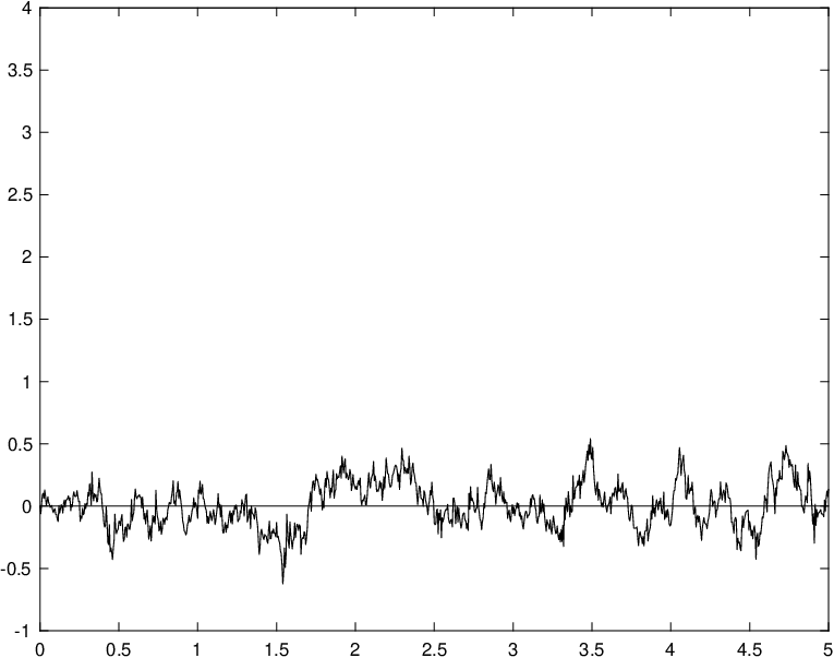
Now, we fix the number of hidden layers and vary the number of units of each layer. The dependence of the DF errors on the number of units for each hidden layer is given in Table 1. In this table, when the observation noise is small, a larger number of units leads to better approximation. On the other hand, when the observation noise is large, this is reversed, i.e., a larger number of units turns out to raise the level of the DF. Kalman filter errors are also included in this table for comparison.
| 3 | 5 | 10 | 20 | KF error | |
|---|---|---|---|---|---|
| 0.1 | 2.60 | 2.44 | 2.27 | 2.10 | 1.70 |
| 0.5 | 5.69 | 5.71 | 4.88 | 4.80 | 4.08 |
| 1.0 | 6.63 | 6.68 | 6.69 | 7.01 | 5.81 |
| 2.0 | 9.33 | 9.46 | 9.59 | 10.59 | 8.23 |
In Table 2, the corresponding CPU times (in seconds) are provided. Overall, as the number of units increases, the required computational time increases. In addition, there appears to be a small decrease in CPU time as observation noise increases.
| 3 | 5 | 10 | 20 | |
|---|---|---|---|---|
| 0.1 | 31 | 45 | 85 | 209 |
| 0.5 | 30 | 45 | 83 | 197 |
| 1.0 | 28 | 40 | 79 | 188 |
| 2.0 | 27 | 39 | 74 | 182 |
Robustness of Deep Filtering
In this section, we examine the robustness of deep filtering. We consider separately the nominal model and the actual model. A nominal model (NM) is an estimated model. It deviates from real data for different applications. In this paper, it is used to train our DNNs, i.e., a selected mathematical model is used to generate Monte Carlo sample paths to train the DNN. The coefficients of the mathematical model are also used in Kalman filtering equations for comparison.
In real world applications, the conversion from real data to mathematical models then Monte Carlo processes can be skipped. Namely, a nominal model consists of actual data to be used to train the DNN directly.
An actual model (AM), on the other hand, is on the simulated (Monte Carlo based) environment. It is used in this paper for testing purposes. In real world applications, the observation process is the actual process obtained from real physical process. To test the model robustness, we consider the case when the NM’s observation noise differs from the AM’s observation noise. In particular, we consider the following two models:
First, with fixed , we vary . The corresponding DF errors and the KF errors are given in Table 3. The KF depends heavily on nominal observation noise. On the other hand, the DF is more robust when . Also, the DF needs the nominal observation noise to be in normal range (not too small) in order to properly train the DNN. Namely, some noise is necessary when training a DNN. Or a noise process in fact helps in the training stage of a DNN.
| 0.1 | 0.5 | 1.0 | 1.5 | 2.0 | 2.5 | |
|---|---|---|---|---|---|---|
| DF | 8.89 | 5.71 | 5.64 | 5.62 | 5.62 | 5.62 |
| KF | 6.54 | 4.08 | 4.59 | 5.33 | 6.04 | 6.70 |
Next, with fixed , we vary . As the actual observation noise increases, both DF and KF deteriorate and the corresponding errors increase as shown in Table 4. The DF appears to be more robust than the KF because it is less sensitive to such changes than the KF.
| 0.1 | 0.5 | 1.0 | 1.5 | 2.0 | 2.5 | |
|---|---|---|---|---|---|---|
| DF | 5.25 | 5.71 | 6.99 | 8.71 | 10.63 | 12.65 |
| KF | 2.90 | 4.08 | 6.49 | 9.15 | 11.88 | 14.59 |
2.2 Nonlinear Models
In this section, we consider nonlinear (NL) models and comparison of the DF with the corresponding extended Kalman filter. We consider the two (NM and AM) models:
We take , step size , and . We also take and . With these specifications, we vary . In Table 5, it can be seen that deep filter is more robust and less dependent on nominal observation noise changes when compared against the corresponding extended Kalman filter. We also note that when training the DF, the observation noise in training data should not be too small. This is typical in DNN training. Too little noise will not provide necessary variations when training the DNN.
| 0.1 | 0.5 | 1.0 | 1.5 | 2.0 | 2.5 | |
|---|---|---|---|---|---|---|
| DF | 12.24 | 7.75 | 7.62 | 7.58 | 7.56 | 7.56 |
| EKF | 9.22 | 5.58 | 6.63 | 8.29 | 10.13 | 12.14 |
Next, we fix and vary , Increasing in actual observation noise will make filtering more difficult and increase the corresponding filtering errors. This is confirmed in Table 6. Also, the DF is less affected than the EKF as increases.
| 0.1 | 0.5 | 1.0 | 1.5 | 2.0 | 2.5 | |
|---|---|---|---|---|---|---|
| DF | 7.01 | 7.75 | 9.68 | 12.22 | 15.01 | 17.89 |
| EKF | 4.19 | 5.58 | 8.62 | 12.26 | 16.17 | 20.07 |
Mixed Nonlinear and Linear Models
In this section, we consider the case when the linearity of the NM and the AM differs. First, we use a linear model to train the DNN while the actual model is in fact nonlinear. In particular, we consider the following two models:
In this case, we fix and vary , The DF is barely affected with the training model (NM) when as shown in Table 7. The dependence of the KF errors on is more pronounced though.
Then we fix and vary . It can be seen from Table 8 that both the KF and DF errors increase in , but the DF is more robust because its errors are less sensitive.
| 0.1 | 0.5 | 1.0 | 1.5 | 2.0 | 2.5 | |
|---|---|---|---|---|---|---|
| DF | 12.91 | 7.75 | 7.61 | 7.57 | 7.56 | 7.56 |
| KF | 9.30 | 5.70 | 6.22 | 7.05 | 7.82 | 8.58 |
| 0.1 | 0.5 | 1.0 | 1.5 | 2.0 | 2.5 | |
|---|---|---|---|---|---|---|
| DF | 7.00 | 7.75 | 9.72 | 12.27 | 15.05 | 17.88 |
| KF | 3.98 | 5.70 | 9.16 | 12.96 | 16.77 | 20.48 |
Finally, we consider the case when the training model is nonlinear while the actual model is linear. We consider the following two models:
Such changes help to improve the filtering outcomes in both DF and EKF when we vary and . It appears that this helps the DF more in reduction of estimation errors as shown in Tables 9 and 10 when compared with Tables 7 and 8, respectively.
| 0.1 | 0.5 | 1.0 | 1.5 | 2.0 | 2.5 | |
|---|---|---|---|---|---|---|
| DF | 8.53 | 5.75 | 5.66 | 5.64 | 5.63 | 5.62 |
| KF | 6.54 | 4.24 | 5.34 | 7.09 | 9.27 | 11.94 |
| 0.1 | 0.5 | 1.0 | 1.5 | 2.0 | 2.5 | |
|---|---|---|---|---|---|---|
| DF | 5.28 | 5.75 | 7.02 | 8.72 | 10.64 | 12.66 |
| KF | 3.12 | 4.24 | 6.55 | 9.13 | 11.80 | 14.50 |
2.3 A Randomly Switching Model
Finally, we consider a switching model with jumps and apply the DF to these models. Note that neither the KF nor the EKF can be used in this case due to the presence of the switching process.
As a demonstration, we consider the following model:
We take to be a continuous-time Markov chain with generator ; see, for example, Yin and Zhang [13] for details. Using step size to discretize to get . We also take and . Two sample paths of , , and the corresponding errors are plotted in Figure 3.


The DF appears to be effective and it catches up quickly the jumps of . Then, in Tables 11 and 12, we provide the errors when one of and is fixed to 0.3 and the other varies. These errors are larger than that of linear and nonlinear models in the previous section mainly because of the presence of jumps. In addition, as moves away from 0.2-0.3, the errors increase. Similarly as in the previous linear and nonlinear models, the errors increase in when is fixed. Overall, the DF shows strong adaptiveness and effectiveness in filtering under highly nonlinear with switching (jumps) dynamic models.
| 0.1 | 0.2 | 0.3 | 0.4 | 0.5 | 0.6 | |
|---|---|---|---|---|---|---|
| DF | 14.88 | 13.41 | 13.78 | 15.05 | 16.33 | 17.72 |
| 0.1 | 0.2 | 0.3 | 0.4 | 0.5 | 0.6 | |
|---|---|---|---|---|---|---|
| DF | 12.22 | 12.74 | 13.78 | 15.19 | 16.82 | 18.59 |
3 Concluding Remarks
In this paper, we developed a new approach using deep learning for stochastic filtering. We explore deep neural networks by providing preliminary experiments on various dynamic models. Naturally one would be interested in any theoretical analysis on related convergence, extensive numerical tests on high-dimensional models with possible high nonlinearity, any genuine real world applications. All in all, this paper raises some opportunities and challenges. Nevertheless, there are more questions than answers.
References
- [1] B.D.O Anderson and J.B. Moore, Optimal Filtering, Prentice-Hall, Englewood Cliffs, NJ, 1979.
- [2] H. A. P. Blom and Y. Bar-Shalom, “The interacting multiple model algorithm for systems with Markovian switching coefficients,” IEEE Trans. Automat. Contr., vol. 33, pp. 780-783, 1988.
- [3] T.E. Duncan, Probability densities for diffusion processes with applications to nonlinear filtering theory and detection theory, PhD Diss., Stanford Univ. (1967).
- [4] F. Dufour, P. Bertrand, and R. J. Elliott, “Filtering for linear systems with jump parameters and high signal-to-noise ratio,” Proc. 13th IFAC World Congress, San Francisco, CA, pp. 445-450, 1996.
- [5] F. Dufour, P. Bertrand, and R. J. Elliott, “Optimal filtering and control of linear systems with Markov perturbations,” Proc. 35th IEEE CDC, Kobe, Japan, pp. 4065-4070, 1996.
- [6] F. Dufour and R. J. Elliott, “Adaptive control of linear systems with Markov perturbations,” IEEE Trans. Automat. Contr., vol. 43, pp. 351-372, 1997.
- [7] O. Hijab, “The adaptive LQG problem -Part I,” IEEE, Trans. Automat. Contr., vol. 28, pp. 171-178, 1983.
- [8] B. M. Miller and W. J. Runggaldier, “Kalman filtering for linear systems with coefficients driven by a hidden Markov jump process,” Systems Control Lett., vol. 31, pp. 93-102, 1997.
- [9] R. E. Mortensen, “Maximum-likelihood recursive nonlinear filtering,” J. Optim. Theory Appl., vol. 2, pp. 386-394, 1968.
- [10] M. Nielsen. Neural networks and deep learning, (online).
- [11] J.J. Kushner, On the differential equations satisfied by conditional probability densities of Markov processes, with applications, J. SIAM Control Ser. A,, vol. 2, pp. 106-119, (1964).
- [12] H.J. Kushner and G. Yin, Stochastic Approximation Algorithms and Applications, Springer, New York, (1997).
- [13] G. Yin and Q. Zhang, Continuous-Time Markov Chains and Applications: A Two-Time Scale Approach, Second Edition, Springer, New York, 2013.
- [14] M. Zakai, On the optimal filtering of diffusion processes, Zeitschrift fur Wahrscheinlichkeitstheorie und Verwandte Gebiete, Vol 11, pp. 230-243, (1969).
- [15] Q. Zhang, “Nonlinear filtering and control of a switching diffusion with small observation noise,” SIAM J. Contr. Optim., vol. 36, pp. 1738-1768, 1998.
- [16] Q. Zhang, Optimal filtering of discrete-time hybrid systems, Journal of Optimization Theory and Applications, Vol. 100, No. 1, pp. 123-144, (1999).
- [17] Q. Zhang, Hybrid filtering for linear systems with non-Gaussian disturbances, IEEE Transactions on Automatic Control, Vol. 45, No. 1, pp. 50-61, (2000).