Generalized -Means in GLMs with Applications to the Outbreak of COVID-19 in the United States
Abstract
Generalized -means can be incorporated with any similarity or dissimilarity measure for clustering. By choosing the dissimilarity measure as the well known likelihood ratio or -statistic, this work proposes a method based on generalized -means to group statistical models. Given the number of clusters , the method is established under hypothesis tests between statistical models. If is unknown, then the method can be combined with GIC to automatically select the best for clustering. The article investigates both AIC and BIC as the special cases. Theoretical and simulation results show that the number of clusters can be identified by BIC but not AIC. The resulting method for GLMs is used to group the state-level time series patterns for the outbreak of COVID-19 in the United States. A further study shows that the statistical models between the clusters are significantly different from each other. This study confirms the result given by the proposed method based on generalized -means.
Key Words: Clustering; COVID-19; Dissimilarity measure; Generalized -means; Generalized information criterion; Generalized linear models (GLMs).
1 Introduction
Generalized -means, including both -means and -medians as special cases, can be incorporated with any similarity or dissimilarity measure to group objects (or observations). The similarity or dissimilarity measure can be very general. In this work, we specify the dissimilarity measure as the well known likelihood ratio or -statistic, such that our method can be used to group statistical models. In particular, if each object contains a vector for the response and a design matrix for the explanatory variables, then statistical models can be used to describe the relationship between the response and explanatory variables within the object. A clustering problem arises if we want to group the statistical models between objects. This problem can be solved by generalized -means. The current research proposes the method and use it to group the state-level time series patterns for the outbreak of COVID-19 in the United States.
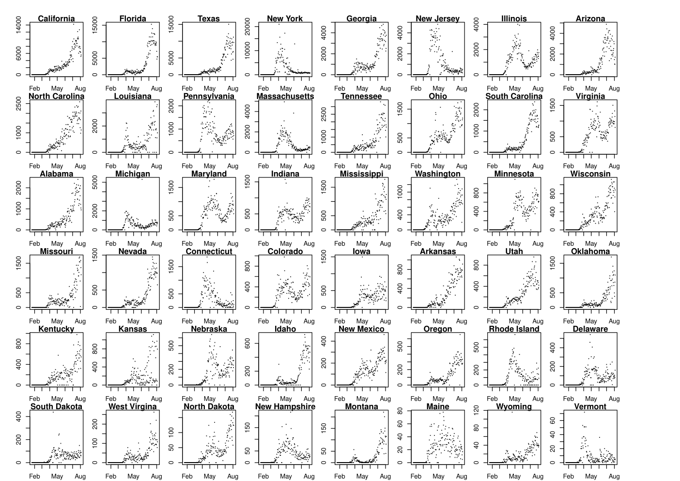
The outbreak of COVID-19 has become a worldwide pandemic since March 2020. According to the website of the World Health Organization (WHO), until July 31, the outbreak has affected over countries with almost eighteen million confirmed cases and seven hundred thousand deaths in the entire world. Among those, the United States has almost five million confirmed cases and one hundred sixty thousand deaths. To understand the outbreak in the United States, we compare the time series patterns for daily new cases in the fifty states and Washington DC. We find that some of the patterns are similar to each other and some of them are far away from each other, implying that we need to have a clustering method to group these patterns. As statistical models are involved, we cannot use traditional -means. We recommend using generalized -means.
Clustering is one of the most popular unsupervised statistical learning methods for unknown structures. Clustering methods are often carried out by a similarity or dissimilarity measure between objects such that they can be grouped into a few clusters. The purpose of clustering is to make objects within clusters mostly homogeneous and objects between clusters mostly heterogeneous. In the literature, one of the most well known clustering methods is the -means. It assigns each object to the cluster with the nearest mean. Based on a given , the -means provides clusters according to centers. The centers are solved by minimizing the sum-of-squares (SSQ) criterion, which is derived based on the Euclidean distance between objects in the data. The SSQ criterion in the -means can be replaced by any similarity or dissimilarity measure. A method called the generalized -means is proposed [1, 27]. Because the choice of the similarity or dissimilarity measure is flexible, generalized -means can be extended to any divergence measure for clustering.
Many clustering methods have been proposed in the literature. Examples include hierarchical clustering [34], fuzzy clustering [29], density-based clustering [18], model-based clustering, and partitioning clustering. Model-based clustering is usually carried out by EM algorithms or Bayesian methods under the framework of mixture models [11, 20]. Partitioning clustering can be interpreted by the centroidal Voronoi tessellation method in mathematics [6]. It can be further specified to -means [10, 14, 21, 22], -medians [2], and -modes [12], where -means is the most popular. To implement those, one needs to express observations of the data in a metric space, such that a distance measure can be defined. Several approaches have been developed to specify the distance measure. A review of these can be found in [17], P 670.

Challenges appear when we want to group the time series patterns for the outbreak of COVID-19 in United States. Suppose that the time series patterns from individual states have been analyzed by statistical models. Then, we need to study the relationship between these models. It is inappropriate to directly compare their coefficients because of disparity. To overcome the difficulty, we recommending using likelihood ratio statistics or an -statistics derived based on hypothesis tests for the relationship between these models, leading to the generalized -means in GLMs. Our method wants to make models within clusters mostly homogeneous and models between clusters mostly heterogeneous. Because of the differences of population sizes, transportation manners, and social activities, the number of daily new cases among the fifty states and Washington DC cannot be identical or even similar, implying that it is inappropriate to compare all of the coefficients. We compare some of the coefficients. This is called the unsaturated clustering problem. In particular, we partition the coefficient vector into two sub-vectors. The first sub-vector does not contain any time information. Therefore, we only need to study the second sub-vector. We implement the generalized -means to the second sub-vector only. This problem can be partially reflected by Figure 1. Suppose that six regression lines are compared. Note that the intercepts do not contain any time information. We allow them to vary within clusters. We restrict the generalized -means on the slopes only, leading to two clusters.
We investigate our method with either a known or an unknown . In the case when is unknown, we propose GIC to select the best . We specify it to BIC and AIC. We find that BIC is more reliable than AIC in selecting the number of clusters. Therefore, we recommend using the BIC selector. We compare our method with a previous method based on the EM algorithm [26]. Our simulation results show that the number of clusters can be identified by our proposed method but not by the previous method. The previous EM algorithm cannot identify the number of clusters if the true number of clusters is greater than two. We implement our method to the state-level time series data for the outbreak of COVID-19 in the United States. We find six clusters.
The article is organized as follows. In Section 2, we propose our method. In Section 3, we study theoretical properties of our method. In Section 4, we evaluate our method with the comparison to a previous method by simulation studies. In Section 5, we implement our method to the state-level COVID-19 data in the United States. In Section 6, we provide a discussion.
2 Method
We propose our method under a given in Section 2.1. It can be combined with GIC [33] to select the best when is unknown. This is introduced in Section 2.2. In Section 2.3, we specify our method to regression models for normal data and loglinear models for Poisson data. The two models will be used in our simulation studies in Section 4. The loglinear model for Poisson data can be extended to a model with overdispersion for quasi-Poisson data. It will be used in clustering for the state-level COVID-19 data in the United States.
2.1 Generalized -Means in GLMs
Clustering is the problem of partitioning a set of objects, denoted by , into several non-empty subsets or clusters, such that the objects within clusters are mostly homogeneous and the objects between clusters are mostly heterogeneous. In the case when the objects can be expressed by points in an Euclidean space, the -means partitions into distinct clusters denoted by with given by
| (1) |
where is the center point of . The right-hand side of (1) is called the SSQ criterion in the -means. The generalized means is proposed if the SSQ criterion is extended to an arbitrary dissimilarity measure. In particular, let be a selected dissimilarity measure with representing an object and representing a cluster. The generalized -means solves by
| (2) |
When are points in an Euclidean space, the generalized -means can be the -means if one chooses . It can also be the -medians if one chooses .
Because is flexible in (2), the generalized -means can be combined with any statistical models. Suppose that is composed by a vector of response and a design matrix of explanatory variables. Then, we can use a statistical model to describe the relationship between the response and the explanatory variables. The response and explanatory variables can be general, implying that the generalized -means can be implemented to various kinds of data, such as text, DNA strains, or images. Here, we restrict our attention to GLMs for continuous or count responses. Our task is to group the GLMs for the objects into a number of clusters.
Suppose that contains a response vector and a design matrix , such that the sample size of the data is . Assume that are independently obtained from an exponential family distribution with the probability mass function (PMF) or the probability density function (PDF) as
| (3) |
where is a canonical parameter representing the location and is a dispersion parameter representing the scale. The linear component is related to explanatory variables by . The link function connects and through
| (4) |
for all and , where is the inverse function obtained by (4). The variance of the response is , where is the variance function of the model. If the canonical link is used, then (4) becomes , implying that is the identity function.
The MLEs of , denoted by , can only be solved numerically if the distribution is not normal. A popular and well known algorithm is the iteratively reweighted least squares (IRWLS) [13]. The IRWLS is equivalent to the Fisher scoring algorithm. It is identical to the Newton-Raphson algorithm under the canonical link. After is derived, a straightforward method is to estimate by moment estimation [24] as
| (5) |
where and is the residual degrees of freedom in the derivation of . If is not present in (3), then (5) is not needed. This occurs in Bernoulli, binomial, and Poisson models. The IRWLS is the standard algorithm for fitting GLMs. It is adopted by many software packages, such as R, SAS, and Python.
Our interest is to determine whether can be grouped into a few clusters, such that there is if objects and are in the same cluster or otherwise. The regression version of this problem has been previously investigated in gene expressions by an EM algorithm [26]. It wants to know whether the entire coefficient vectors can be partitioned into a few clusters. In our method, we allow a few components of to be different within clusters, such that we only need to partition the objects based on the rest components.
Suppose that (4) is expressed as
| (6) |
where and . We want to know whether can be grouped into a few clusters. It means that we want if objects and are in the same cluster or otherwise. Based on a given , the clustering model in our method is
| (7) |
for . We call (7) the unsaturated clustering problem. If is absent, it becomes the saturated clustering problem, the problem studied by [26]. As the choice of and is flexible in (7), our method can be used to group GLMs based on any sub-vectors of . We use either a likelihood ratio statistic or an -statistic to construct in (2).
Our method starts with a set of cluster candidates , which can be any partition of . For any given and , if , we directly use and in the derivation of ; otherwise, we remove from in the derivation. Then, the resulting does not contain . We obtain the likelihood ratio statistic or the -statistic for
| (8) |
The likelihood ratio statistic is used if is absent in (3). This appears in Poisson and binomial models. The -statistic is used if is present. This appears in normal models. For each and , we calculate the -value of the likelihood ratio statistic or the -statistic. We assign to the cluster candidate with the largest -value. Then, we obtain the updated set of cluster candidates, which is used in the next iteration. To ensure non-empty, we do not move the object with the largest -value in to any other cluster candidates. We have the following algorithm.
Algorithm 1 has two major stages. The second stage is given by Step 2 to Step 5, which is common in many -means algorithms. Therefore, we only discuss the first stage, which is given by Step 1. The goal of the first stage is to find the best initial . We do not use the usual approach adopted by many -means algorithms, as they select the initial set of cluster candidates randomly. Instead, we want to make the initial as heterogeneous as possible. At the beginning, we randomly choose the first from . We denote it as . It is the seed for . We calculate the -value of the likelihood ratio statistic or the -statistic for
| (9) |
for every . The object with the lowest -value is chosen the seed for . It is denoted by . Then, we incorporate the minimax principle to select the rest seeds. Suppose that and are selected. For each , we calculate the -values of the likelihood ratio statistic or the -statistic based on two testing problems as
| (10) |
where the two testing problems are derived by taking and , respectively. We obtain two -values. We assign the maximum of the two -values as the -value of . The object with the lowest -value is chosen as the seed for . It is denoted by . Using this idea, we can obtain all the seeds . Then, we reconsider the testing problem given by (10). For a given with , we calculate the -values of the likelihood ratio statistic or the -statistic for all . We assign to if the -value is maximized at . After doing this for all the rest objects, we obtain the initial . Combining it with the second stage, we obtain non-empty clusters with the corresponding value and -value of the likelihood ratio statistic or the -statistic.
2.2 Generalized Information Criterion
The generalized -means introduced in Section 2.1 cannot be used if is unknown. As the likelihood function is provided in Algorithm 1, we can used it to define a penalized likelihood function. It is used to determine the number of clusters if is unknown. The penalized likelihood approach has been widely applied in variable selection problems. Here, we adopt the well known GIC approach [33] to construct our objective function. The best is obtained by optimizing the objective function.
Let be the loglikelihood of (7), where represents all of the parameters involved in the model. If the dispersion parameter is not present, then is composed by and for all and only. It is enough for us to use to define the objective function in GIC. If the dispersion parameter is present, then we need to address the impact of estimation of , because variance can be seriously underestimated in the penalized likelihood approach under the high-dimensional setting [7]. We decide to introduce our approach based on (3) without . We then propose a modification when it is present.
Assume that does not appear in (3). The GIC for (7) is defined as , where is the MLE of and is the model degrees of freedom under , and is a positive number that controls the properties of GIC. Let be the dimension of and be the dimension of . Then, . Note that does not vary with . We define the objective function in our GIC as
| (11) |
The best is solved by
| (12) |
where is the best grouping based on the current . The GIC given by (11) includes AIC if we choose or BIC if we choose . If they are adopted, then the solutions given by (12) are denoted by and , respectively.
We need to estimate the dispersion parameter if it is present. Because the estimator based on the current can be seriously biased, we recommending using as the number of clusters in the computation of the estimate of . In particular, we calculate the best based on the current in the generalized means. We use it to compute and for all and . Then, we calculate the best by setting the number of clusters equal to . We use (5) to estimate . This is analogous to the full model versus the reduced model approach in linear regression, where the variance parameter is always estimated under the full model. We treat the model with clusters in (7) as the full model, and the model with clusters as the reduced model. We estimate based on the full model but not the reduced model. After is derive, we put it into (11) in the computation of GIC. We then use (12) to calculate the best with the dispersion parameter. This is important in our method for regression models.
2.3 Specification
We specify our method to regression models for normal data and loglinear models for Poisson data. Ordinary regression models are commonly used if the interest is to discover the relationship between a single continuous response variable and a number of explanatory variables. Multivariate regression models are commonly used if at least two continuous response variables are involved. Loglinear models for Poisson data and logistic linear models for binomial data are commonly used if the response is count. They have been extended to quasi-Poisson or quasi-binomial models to incorporate overdispersion.
In ordinary regression models, (6) becomes
| (13) |
where , , and . With a given , the model in our generalized -means becomes
| (14) |
for . We treat (14) as a special case of (13). The second stage in Algorithm 1 is common. We only focus on the first stage.
We select seed for randomly. Suppose that have been selected as the seeds for , for any , respectively. To determine the seed for , we calculate the dissimilarity measure between and for pairs with and based on
| (15) |
where or , is the dummy variable defined as if or if , and is the error vector. We calculate the -statistic for
| (16) |
Let be the -value of the -statistic. We define the -value of the dissimilarity between and as
| (17) |
We choose as the seed of if it has the lowest value among all objects in . Therefore, is given by the minimax principal as
| (18) |
After we obtain , the set of all of the seeds for , we calculate the -value of the -statistic for (16) for every and . We assign to if is maximized at . In the end, we obtain the initial . By iterating the second stage in Algorithm 1, we obtain based on a given .
Because of the presence of , we follow the GIC in variable selection for regression models [33], and propose our GIC in the generalized -means for regression models as
| (19) |
where is the sum of squares of errors given by (14). To implement (19), we need to estimate . If the current is used, then the estimate of is divided by residual degrees of freedom. The first term on the right-hand side of (19) is always equal to , implying that we cannot use this approach to select the best . To overcome the difficulty, we recommend using in (14) in estimating . We denote it by . Therefore, our GIC is
| (20) |
where is the SSE with clusters in (14). This is appropriate. If the number of true clusters is less than or equal to , then slightly increasing the number of clusters by would not significantly change the estimate of , implying that the second term dominates the right-hand side of (20). Otherwise, the estimate of would be significantly reduced, implying that the first term dominates the right-hand side of (20). Therefore, the objective function in our GIC provides a nice trade-off between the SSE and the penalty function.
For Poisson data, there is , implying that . Under the framework of loglinear models, (6) becomes
| (21) |
With a given , it reduces to
| (22) |
for . Analogous to the regression models, after selecting randomly, we investigate
| (23) |
with or . We measure the dissimilarity between and by the likelihood ratio statistic for (16). We derive the initial by the same idea that we have displayed in regression models. With the second stage in Algorithm 1, we obtain based on a given . To determine the best , we choose as the residual deviance of (22). As the dispersion parameter is not present, the implementation of GIC is straightforward.
For quasi-Poisson data, there is , implying that . We can still use (21), (22), and (23) to find the best . To determine the best , we estimate by (5), which is the Pearson goodness-of-fit given by (22) divided by its residual degrees of freedom. For the same reason, we choose the number of clusters equal to in (22) in estimating . We denote it by , leading to
| (24) |
where is the residual deviance (i.e., deviance goodness-of-fit) with clusters in (22).
3 Asymptotic Properties
We evaluate the asymptotic properties of our method under . It is achieved by letting . To simplify our notations, we assume that are all equal to and are all equal to such that we have and in our data. The case with distinct and can be proven under their minimums tend to infinity with bounded ratios between the minimums and the maximums.
The asymptotic properties are evaluated under with . For any , let be the likelihood ratio statistic for
| (25) |
As , is asymptotically distributed if and are in the same cluster, or goes to with rate otherwise. Because (25) is applied to all pairs in , the multiple testing problem must be addressed. This can be solved by the method of higher criticisms [5].
Lemma 1
Assume that for are iid copies from (7) for any given . If and are in the same cluster, then . If and are in different clusters, then exists a positive constant , such that the limiting distribution of is non-degenerate as .
Proof. The conclusion can be proven by the standard approach to the asymptotic properties of maximum likelihood and M-estimation. Please refer to Chapter 22 in [9] and Chapter 5 in [30].
Theorem 1
If the assumption of Lemma 1 holds, and for some when , then .
Proof. Note that the likelihood ratio test based on is applied to distinct . We need to evaluate the impact of the multiple testing problem. We examine the distribution of the based on Lemma 1. According to [5], it is asymptotically bounded by a constant times if and are in same clusters or increases to with rate if and are in different clusters. Thus, with probability , the increasing rate of with and in different clusters is faster than that of with and in same clusters, implying the conclusion.
Theorem 2
Proof. If , then we can find at least one pair of and , such that they are not in the same cluster but they are grouped to the same cluster. By Lemma (1), the first term on the right-hand side of (11) goes to with rate . It is faster than the rate of GIC under , implying that as . Therefore, we only need to study the case when . Note that the loglikelihood function of (7) based on a given is equal to the sum of the loglikelihood functions obtained from each . By Theorem 1, we can restrict our attention to the case when all objects in are in the same cluster. By [5], with probability , the loglikelihood function (7) in is not higher than that under the true cluster plus . By the property of the -approximation of the likelihood ratio statistic under the true , we have that with probability the first term on the right-hand side of (11) is not higher than . Combining it with the second term, we conclude that . We obtain the first conclusion. Then, we draw the second conclusion by Theorem 1.
Theorem 1 implies that both and can increase exponential fast than if is known, but the rate is significantly reduced if is unknown. If , then we cannot choose in our method, implying that is not consistent, but we can still show that is consistent.
Corollary 1
Suppose that all of assumptions of Theorem 2 are satisfied. If or is constant, and when , then .
Proof. Note that the increasing rate of cannot be lower than the increasing rate of . We draw the conclusion by Theorem 2.
4 Simulation
We carried out simulations to evaluate our methods. For an estimated cluster assignment and the true clustering assignment , we define the clustering error () of as
| (26) |
where if and belong to the same clusters in , or otherwise, and similarly for in . For estimated clustering assignments obtained from simulation replications, respectively, we calculate the percentage of clustering object errors () by
| (27) |
This is a commonly used criterion in the clustering literature [31]. We also study the percentage of number of clusters identified correctly () as
| (28) |
where are the numbers of clusters obtained from simulation replications, respectively, and is the true number of clusters. We compare clustering methods based on and .
4.1 Regression Models
We established regression models with clusters. Each cluster had objects. Each object contained observations. We generated explanatory variables from and from independently. For each selected , , and , we generated the normal response from
| (29) |
for and , where with was the random error. We evaluated our methods based on AIC and BIC with the comparison to the previous EM algorithm method proposed by [26]. To implement the EM algorithm, we only considered the saturated clustering problem, where we set not varied within clusters. We made if and were in the same cluster in (29). If , we chose , , and if was in the first cluster or , , and if was in the second cluster. If , we added one more cluster with , , and if was in the third cluster. Then, we could generate data from (29) with either or clusters.
| EM | AIC | BIC | EM | AIC | BIC | |||
|---|---|---|---|---|---|---|---|---|
Table 1 displays the simulation results for the percentage of clustering number errors with respect to the previous EM algorithm, and our AIC and BIC selectors. In all of the simulations that we ran, we found that the number of clusters reported by the EM algorithm was either or , implying that it could not find the correct number of clusters if . The true could be detected by our BIC not our AIC.
| EM | BIC | EM | BIC | EM | BIC | EM | BIC | ||
|---|---|---|---|---|---|---|---|---|---|
Table 2 displays the simulation results for the percentage of clustering object errors based on the previous EM algorithm and our BIC selector. We did not include AIC in the table because it could not detect the correct . Our result shows that BIC in the generalized -means was always better that in the previous EM algorithm. Our BIC was able to find the true number of clusters with lower clustering object errors. The previous EM algorithm cannot be used to study the unsaturated clustering problem. This is an advantage of our generalized -means.
4.2 Loglinear Models
Similar to the regression models, we also chose clusters in loglinear models for Poisson data. Each cluster had objects. Each object contained observations. We generated explanatory variables and from independently. For each selected , , and , we independently generated the response from with
| (30) |
for and . We generated independently from . We set in the first cluster and in the second cluster. This was used if . If , we chose in the third cluster. We evaluated our method based on AIC and BIC for the unsaturated clustering problem, where we varied within clusters.
| AIC | BIC | AIC | BIC | AIC | BIC | AIC | BIC | ||
|---|---|---|---|---|---|---|---|---|---|
Table 3 displays the simulation results for the percentage of clustering number errors. We also found that the true could be identified by our BIC but not by our AIC. Table 4 displays the results for the percentage of clustering object errors based on BIC. It shows that the percentage of clustering object errors was still low, indicating that BIC can be used to find the correct number of cluster with the low error rate. Therefore, we recommend using BIC in our generalized -means if the number of clusters is unknown.
| for | for | ||||
|---|---|---|---|---|---|
5 Application
We implemented our method to the state-level COVID-19 data in the United States. It is known that the outbreak of COVID-19 in the world has occurred in March 2020 and more than countries have affected. The situation in the United States is the most serious in the world. Until July 31, the United States has over million confirmed cases and one hundred sixty thousand deaths, which are the highest in the world. After briefly looking at the data (Figure 2), we found significant changes in the time series patterns before May 31 and after June 1. We suspected two possible reasons from social medias. The first was the George Floyd issue, occurred on May 25 in Minneapolis. The second was the economy reopening issue. Most states reopened their economy or released their restrictions for the spread of the infection at the end of May. Therefore, we needed to pay attention to their impacts in the implementation of our method.
It is known that the first patient of COVID-19 appeared in Wuhan, China, on December 1 2019. In late December, a cluster of pneumonia cases of unknown cause was reported by local health authorities in Wuhan with clinical presentations greatly resembling viral pneumonia [3, 28]. Deep sequencing analysis from lower respiratory tract samples indicated a novel coronavirus [8, 15]. The virus of COVID-19 primarily spreads between people via respiratory droplets from breathing, coughing, and sneezing [32]. This kind of spreading can cause cluster infections in society. To avoid cluster infections, many countries have imposed travel restrictions. These restrictions have affected over of the total population of the world with three billion people living in countries with restrictions on people arriving from other countries borders completely closed to noncitizens and nonresidents [25].
Exponential increasing trends are expected at the beginning of outbreaks of any infectious disease. This phenomenon has been observed in the 2009 Influenza A (H1N1) pandemic [4] and the 2014 Ebola outbreak in West Africa [16]. Without any prevention efforts, the exponential trend will be continuing for months until a large portion of people are infected, but this can be changed due to prevention by governments [23].
To obtain a more appropriate model for the time series patterns in the United States, we investigate a few candidate models. We choose the response as the number of daily new cases and explanatory variables as functions of time. We find that two models were useful. The first is the exponential model as
| (31) |
where is the starting date, is the current date, , and is the number of daily new case observed on the current date. The second is the Gamma model given as
| (32) |
It assumes that the expected value of number of daily new cases is proportional the density of a Gamma-distribution. If the second term is absent, then the Gamma model becomes the exponential model, implying that (31) is a special case of (32).
| Exponential | Gamma | |||||||
|---|---|---|---|---|---|---|---|---|
| Country | Peak | |||||||
| China | 02/07 | |||||||
| USA | 04/26 | |||||||
| Canada | 04/26 | |||||||
| Russia | 05/13 | |||||||
| Spain | 04/08 | |||||||
| UK | 04/22 | |||||||
| Italy | 04/03 | |||||||
| France | 04/07 | |||||||
| Germany | 04/05 | |||||||
| Switzerland | 03/30 | |||||||
| Sweden | 04/30 | |||||||
Suppose that . If , then the third term dominates the variation of the right-hand side of (32). The expected value of the response goes to infinity as time goes to infinity, leading to an exponential increasing trend. If , then the peak of the model is . An increasing trend is expected if and a decreasing trend is expected otherwise. Therefore, we can use the sign of to determine whether the outbreak is under control or out of control.
We chose as January 11 in both (31) and (32). We assumed that followed the quasi-Poisson model, such that we could fit the two models by the traditional loglinear model with the dispersion parameter to be estimated by (5). We assessed the two models by their values, where the value of a GLM was defined as one minus residual deviance divided by the null deviance. We verified (31) and (32) by implementing them to eleven countries in the world (Table 5), where the peak was estimated by with and as the MLEs of and in the model. We found that the results given by the Gamma model were significantly better than those given by the exponential model.

We established our generalized -means clustering under (32) to group the states and Washington DC. The model was
| (33) |
where , was the number of daily new cases from the th state on the th date, and and were the coefficients given by the th cluster.
We looked at the state-level data and found that many of daily new cases were zeros in January and February. This was because the United States only had total number of confirmed cases until February 24. We decided to exclude data before February 24 in the analysis. We applied (33) to the data between February 24 and May 31 and the data between February 24 and July 31, respectively. We compared their difference to evaluate the impact of the two issues that we mentioned at the beginning of this section. We obtained six clusters based on the BIC approach (Figure 3).
To verify our clustering result, we examined three models. The first was the main effect model. It had only one cluster in (33). The second was the resulting (33) with clusters. The third was the interaction effect model. It assumed that each state formed a cluster in (33). We calculated the differences of residual deviance between the first and second models, and between the first and the third models, respectively. We obtained the partial value by the ratio of the two differences. The partial value interpreted the ratio of residual deviance reduced by the model with clusters. When , we obtained that the partial was for data between February 24 and May 31, and for data between February 24 and July 31, implying that the model with six clusters was good enough for the differences among the states and Washington DC.
| 02/24–05/31 | 02/24–07/31 | |||||||
|---|---|---|---|---|---|---|---|---|
| Cluster | State | Peak | State | Peak | ||||
| California | 5/10(2.27) | California | ||||||
| New York | 4/3(0.28) | New York | 4/12 | |||||
| Illinois | 4/28(0.81) | Illinois | 5/11 | |||||
| Louisiana | 4/8(0.39) | Louisiana | ||||||
| Minnesota | 5/17(7.3) | Minnesota | 6/5 | |||||
| Florida | 4/26(0.42) | Florida | ||||||
We evaluated properties of identified clusters by the MLEs of and with in (33) with (Table 6). We found the situation in the entire United States was under control before May 31 as the signs of were all negative. The situations in the states contained by the first, the fourth, and the six clusters became worse, but the situations in the states contained by the second, the third, and the fifth clusters were still under control. The change was probably caused by that a lot of people did not keep social distance or did not stay at home in June and July in the United States.
6 Discussion
We have proposed a new clustering method under the framework of the generalized -means to group statistical models. The method can automatically select the number of clusters if it is combined with the GIC approach. We study BIC and AIC, which are two popular special cases in GIC. Our theoretical and simulation results show that the correct number of clusters can be identified by BIC but not by AIC. Therefore, we recommend using BIC to find the number of clusters if is unknown. We implement our method to partition loglinear models for the state-level COVID-19 data in the United States and finally we have identified six clusters. An important advantage is that our method can be used to study the unsaturated clustering problem, which is different from the saturated clustering problem studied by traditional -means or -medians. As the choice of the dissimilarity measure is flexible, our method can be extended to many scenarios beyond GLMs. This is left to future research.
References
- [1] Bock, H. (2008) Origins and extensions of the k-means algorithm in cluster analysis Electron. Electronic Journal for History of Probability and Statistics, 4, Article 14.
- [2] Charikar, M., and Guha, S. (2002). A constant-factor approximation algorithm for the -median problem. Journal of Computer and System Science, 65, 129-149.
- [3] Chen, N., Zhou, M., Dong, X., Qu, J., Gong, F., Han, Y., Qiu, Y., Wang, J., Liu, Y., Wei, Y., Xia, J., Yu, T., Zhang, X., and Zhang, L. (2020). Epidemiological and clinical characteristics of 99 cases of 2019 novel coronavirus pneumonia in Wuhan, China: a descriptive study. The Lancet, 395, 507-513.
- [4] de Picoli, S., Teixeira, J.J., Ribeiro, H.V., Malacarne, L.C., dos Santos, R.P., dos Santos Mendes, R. (2011). Spreading patterns of the influenza A (H1N1) pandemic. PLOS ONE, 6, e17823.
- [5] Donoho, D., and Jin, J. (2004). Higher criticism for detecting sparse heterogeneous mixtures. Annals of Statistics, 32, 962-994.
- [6] Du, Q., and Wong, T.W. (2002). Numerical studies for MacQueen’s -means algorithms for computing the centroidal Voronoi tessellations. Computer and Mathematics with Applications, 44, 511-523.
- [7] Fan, J., Guo, S., and Hao, N. (2012). Variance estimation using refitted cross-validation in ultrahigh dimensional regression. Journal of Royal Statistical Society Series B, 74, 37-55.
- [8] Feng, Z. (2020). Urgent research agenda for the novel coronavirus epidemic: transmission and non-pharmaceutical mitigation strategies. Chinese Journal of Epidemiology, 41, 135-138.
- [9] Ferguson, T.S. (1996). A Course in Large Sample Theory. CRC Press, New York.
- [10] Forgy, E. W. (1965). Cluster analysis of multivariate data: efficiency vs interpretability of classifications. Biometrics, 21, 768–769.
- [11] Fraley, C. and Raftery, A.E. (2002). Model-based clustering, discriminant analysis, and density estimation. Journal of the American Statistical Association, 97, 611-631.
- [12] Goyal, M., and Aggarwal, S. (2017). A review on -mode clustering algorithm. International Journal of Advanced Research in Computer Science, 8, 725-729.
- [13] Green, P.J. (1984). Iteratively reweighted least squares for maximum likelihood estimation, and some robust and resistant alternative. Journal of Royal Statistical Society Series B, 46, 149-192.
- [14] Hartigan, J. A. and Wong, M. A. (1979). A -means clustering algorithm. Applied Statistics, 28, 100–108.
- [15] Huang, C., Wang, Y., Li, X., Ren, L., Zhao, J., Hu., Y., Zhang, L., Fan, G., Xu, J., Gu., X., Cheng, Z., Yu, T., Xia, J., Wei, Y., Wu., W., Xie, X., Yin, W., Li, H., Liu, M., Xiao, Y., Gao, H., Guo, L., Xie, J., Wang, G., Jiang, R., Gao, Z., Jin, Q., Wang, J., Cao, B. (2020). Clinical features of patients infected with 2019 novel coronavirus in Wuhan, China. The Lancet, 395, 497-506.
- [16] Hunt, A.G. (2014). Exponential growth in Ebola outbreak since May 14, 2014. Complexity, 2̱0, 8-11.
- [17] Johnson, R.A. and Wichern, D.W. (2002). Applied Multivariate Statistical Analysis. Prentice Hall, New Jersey.
- [18] Kriegel, H.P., Kröger, P., Sander, J., and Zimek, A. (2001). Density-based clustering. WIRES Data Mining Knowledge Discovery, 1, 231-240.
- [19] Kwedlo, W. (2011). A clustering method combing differential evolution with the -means algorithm. Pattern Recognition Letters, 32, 1613-1621.
- [20] Lau, J.W. and Green, P.J. (2007). Bayesian model-based clustering procedures. Journal of Computational and Graphical Statistics, 16, 526-558.
- [21] Lloyd, S.P. (1982). Least squares quantization in PCM. IEEE Transactions on Information Theory, 28, 128–137.
- [22] MacQueen, J. B. (1967). Some Methods for classification and Analysis of Multivariate Observations. Proceedings of 5th Berkeley Symposium on Mathematical Statistics and Probability. University of California Press. pp. 281–297.
- [23] Maier, B.F. and Brockmann, D. (2020). Effective containment explains subexponential growth in recent confirmed COVID-19 cases in China. Science, DOI: 10.1126/science.abb4557.
- [24] McCullagh, P. (1983). Quasi-likelihood functions. Annals of Statistics, 11, 59-67.
- [25] Pew Research Center (2020). More than nine-in-ten people worldwide live in countries with travel restrictions amid COVID-19. https://www/pewreseach.org/fact-tank/2020/04/01
- [26] Qin, L.X. and Self, S.G. (2006). The Clustering of regression models method with applications in gene expression data. Biometrics, 62, 526-533.
- [27] Soheily-Khah, S., Douzal-Chouakria, A., and Gaussie, E. (2016). Generalized -means-based clustering for temporal data under weighted and kernel time warp. Pattern Recognition Letters, 75, 63-69.
- [28] Sun, K., Chen, J., and Viboud, C. (2020). Early epidemiological analysis of the coronavirus disease 2019 outbreak based on crowdsourced data: a population-level observational study. The Lancet Digital Health.
- [29] Trauwaert, E., Kaufman, L., and Rousseeuw, P. (1991) Fuzzy clustering algorithms based on the maximum likelihood principle. Fuzzy Sets and Systems, 42, 213-227.
- [30] van der Vaart, A.W. (1998). Asymptotic Statistics, Cambridge University Press, Cambridge, UK.
- [31] Wang, J. (2010). Consistent selection of the number of clusters via cross validation. Biometrika, 97, 893-904.
- [32] World Health Organization (WHO) (2020). Getting your workplace ready for COVID-19. February 27 2020.
- [33] Zhang, Y., Li, R., and Tsai,, C. (2010). Regularization parameter selections via generalized information criterion. Journal of the American Statistical Association, 105, 312-323.
- [34] Zhao, Y. and Karypis, G. (2005). Hierarchical clustering algorithms for document datasets. Data Mining and Knowledge Discovery, 10, 141-168.