Numerical Methods for a Diffusive Class Nonlocal Operators Thanks: This work is supported in part by the National Science Foundation under grant DMS-1911742 (GJ).

Loic Cappanera Email: lmcappan@central.uh.edu, gabriela@math.uh.edu, cward7@central.uh.edu Thanks: Department of Mathematics, University of Houston, Houston, TX (). Gabriela Jaramillo¹¹footnotemark: 1 Cory Ward¹¹footnotemark: 1

Abstract

In this paper we develop a numerical scheme based on quadratures to approximate solutions of integro-differential equations involving convolution kernels, $\nu$ , of diffusive type. In particular, we assume $\nu$ is symmetric and exponentially decaying at infinity. We consider problems posed in bounded domains and in $\mathbb{R}$ . In the case of bounded domains with nonlocal Dirichlet boundary conditions, we show the convergence of the scheme for kernels that have positive tails, but that can take on negative values. When the equations are posed on all of $\mathbb{R}$ , we show that our scheme converges for nonnegative kernels. Since nonlocal Neumann boundary conditions lead to an equivalent formulation as in the unbounded case, we show that these last results also apply to the Neumann problem.

keywords

nonlocal diffusion operator, integro-differential equations, finite difference method, numerical approximation, convergence analysis.

AMS

41A55 (approximate quadratures), 45A05 (linear integral equations), 45J05 (integro-differential equation), 45P05 (integral operators), 65R20 (numerical methods for integral equations).

1 Introduction

In this paper we are interested in developing numerical algorithms for approximating nonlocal evolution processes of the form

u_{t}(x,t)=\int_{\mathbb{R}}(u(y,t)-u(x,t))\nu(x,y)\;dy+f(x),\quad x\in\Omega\subset\mathbb{R},

(1)

where $\nu(x,y)=\nu(|x-y|)$ is a symmetric, extended (no compact support), and exponentially decaying function of diffusive type, which is not necessarily positive.

Integro-differential equations like the one above appear, for example, as model equations for diffusion processes that occur over fast time scales. They can be derived by first considering a reaction diffusion system, and then using a Green’s function to approximate the fast variable in terms of the slow variables. The result is a nonlocal equation (or system) involving a convolution kernel. This kernel describes a dispersion processes that lies somewhere between regular diffusion, as expressed by the Laplace operator, and anomalous diffusion, modeled for instance using the Fractional Laplacian. More precisely, when viewed as probability density functions for a random walk, the kernels considered here have finite second moment. Generally, this implies that the process has a characteristic length scale, and one might be tempted to switch the convolution kernel for the Laplace operator with an appropriate diffusion constant. However, as has been shown (see for example [39, 40, 29, 7, 24]) this simplification misses the true character of the fast diffusion process and precludes one from finding interesting behavior, like for example chimera states [39].

Other examples of systems that can be described using equation (1) come from population dynamics [38, 34, 13], and oscillating chemical reactions [45, 39, 28]. Variations of the above integro-differential equation also appear in other physical systems where nonlocal effects are important. For instance, the references [3, 37, 17, 9, 8] explore a nonlocal continuum model for phase transitions, and in [11] a model for the evolution of a particle system is presented. Peridynamic models also give rise to integro-differential equations like the ones studied here, although in this case the convolution kernel is often assumed to have compact support. These models have been the subject of large study and are one of the driving forces behind the development of numerical schemes for nonlocal models, [41, 44, 43, 6, 48, 42, 36, 10, 14, 49, 47]. Finally, extensions of the above equation in which the integral operator is nonlinear, are also typical of neural field models. In this case, the linearization about the homogenous steady state has the form of equation (1), see for example [4, 25, 12] and [15]. Of course, the literature presented here is not exhaustive and is just meant to give a general idea of the breath of applications that use nonlocal models.

Although in most applications the set $\Omega$ represents a physical domain that is bounded, when the phenomenon of interest occurs at small spatial scales compared to the size of this domain, it is reasonable to pose the equation on all of $\mathbb{R}$ . This is the case for example when showing existence of traveling waves in predator prey models [16], or existence of target patterns solutions in oscillating chemical reactions [32]. On the other hand, when both scales are comparable and $\Omega$ is considered to be a bounded subset of $\mathbb{R}$ , boundary conditions need to be formulated carefully. Given that the model is now described by an integro-differential equation, it is not enough to prescribe the value of the solution or its derivatives at the boundary. Instead, boundary conditions take the form of volume constraints, see [19, 20]. Indeed, in various applications volume constraints can provide an equivalent notion to Dirichlet and Neumann boundary conditions that, moreover, is consistent with the assumptions made in deriving evolution equations of the form (1). See also the discussion in Appendix A.

In both cases, bounded and unbounded $\Omega$ , one is interested in validating and guiding the mathematical analysis using numerical simulations. Currently, one approach to approximate equation (1) is to use an exponential time difference scheme, [33]. This consists in picking a large domain, applying the Fourier transform to the spatial variable, and then using an RK4 method to advance the time steps while computing any nonlinearities in real space. One of the disadvantages of this approach is that the implied periodic boundary conditions are not always desired. Moreover, computations can become costly if one also needs a small spatial discretization to resolve small scale phenomena. Alternatively, if the kernel $\nu(x,y)$ has as its Fourier symbol a fractional polynomial, then it is possible to precondition the equation with an appropriate differential operator and obtain as a result a PDE, see for example [35]. One can then proceed to solve the problem using finite differences, and impose local Dirichlet or Neumann boundary conditions. The main draw back from this approach is that the type of convolution kernels one can consider is restricted.

The goal of this paper is to propose a numerical method based on quadratures for computing steady states,

\int_{\mathbb{R}}(u(x,t)-u(y,t))\nu(|x-y|)\;dy=f(x),\quad x\in\Omega\subset\mathbb{R}.

(2)

which, in contrast to the methods mentioned above, accounts for nonlocal boundary conditions. In particular, we provide schemes for approximating solutions to (2) when

i)

$\Omega\subset\mathbb{R}$ is bounded and we know the value of the solution in $\Omega^{c}$ .
ii)

$\Omega=\mathbb{R}$ and we assume the algebraic decay of the solution.
iii)

$\Omega\subset\mathbb{R}$ is bounded and we know the algebraic decay of the solution and the nonlocal flux from $\Omega^{c}$ into $\Omega$ .

Our scheme is adapted from [30], where the authors look at item i) in the particular case when $\nu(|x-y|)$ is the integral kernel associated with the Fractional Laplacian, $(-\Delta)^{\alpha/2}$ , $0<\alpha<2.$ Our main contribution is to extend this scheme and provide a proof of convergence for all three problems (i)-(ii)-(iii) for a larger range of kernels, meaning kernels that satisfy Hypotheses 3.2 and 3.3 and that are therefore exponentially decaying and do not have compact support. Moreover, in the case of problems with nonlocal Dirichlet boundary conditions, kernels are allowed to take negative values.

Notice that the properties exhibited by our kernels are in direct contrast to those considered in most of the literature pertaining to the numerical approximation of nonlocal equations. Indeed, most numerical schemes deal with either the integral form of the factional Laplacian, [30, 2, 1, 21, 22] or with nonlocal operators involving kernels that are positive and compactly supported [23, 47, 20, 46, 18]. In addition, since the problems considered here are posed on the whole real line, there are additional difficulties not encountered when looking at bounded domains with, for example, Dirichlet boundary conditions, or at problems that involve positive kernels with compact support. Mainly the issue to be addressed is how to approximate the solution outside the computational domain. On the other hand, from a theoretical point of view it is not immediately clear that solutions exists and are unique when problem (2) is posed on all of $\mathbb{R}$ . The second main contribution of this paper is to adapt previous results from [32] to show that the assumption of algebraic decay for solutions to equation (2) leads to a well posed problem, provided that the right hand side, $f$ , also has sufficient decay and satisfies some compatibility conditions (zero mean and zero first moment).

Our results are organized as follows. In Section 2, we present the different nonlocal diffusion problems and boundary conditions that are considered in this paper. Details on the derivation of the equation (1), as a model for population dynamic, and how nonlocal Dirichlet and Neumann boundary condition can be naturally defined are provided in Appendix A. In Section 3, we prove that the nonlocal problem (2) is well posed if the equation is defined on a particular class of weighted Sobolev spaces. In particular, we derive conditions on the right hand side, $f$ , that guarantee existence of a unique solution. These results hold for a large class of kernels, and for problems defined either on the whole real line or on bounded domains with nonlocal Neumann boundary condition. In this section we also state conditions that guarantee the problem is well posed when considering nonlocal Dirichlet boundary conditions. In Section 4 we adapt the methods from [30] to the problems i), ii) and iii). The convergence of the numerical schemes is established in Section 5. Unlike most schemes proposed in literature, the convergence of the Dirichlet problem is established for kernels that can take negative values assuming the kernel has a positive tail. Finally, in Sections 6.1, 6.2, and 6.3 we provide examples for cases i), ii), and iii), respectively.

2 Nonlocal diffusion model and boundary conditions

As mentioned in the introduction, the derivation of equations (1) and (2) has been done in various contexts, see again for example [5, 19, 20, 27]. In the case of diffusion problems, the key idea is to extend the concept of flux across a boundary to a version of flux that includes short as well as long range movement of particles. This extension is explained in detail in references [19, 20]. For completeness, in Appendix A we summarize some of the results of the above references, and use an example from populations dynamics to derive equation (1).

In this paper, we concentrate on the 1-dimensional steady state problem with nonlocal diffusion operator $\mathcal{L}$ of the form:

\mathcal{L}\ast u=\int_{\mathbb{R}}(u(x,t)-u(y,t))\nu(x,y))\;dy,

where the kernel $\nu$ is assumed to be symmetric, meaning that $\nu(x,y)=\nu(|x-y|)$ , and exponentially decaying. We study three types of problems that are either defined on a bounded domain $\Omega$ with nonlocal Dirichlet or Neumann boundary conditions, or defined on the whole real line $\mathbb{R}$ . These problems can be described as follows:

•

Dirichlet boundary conditions

$\begin{array}[]{c c c}\mathcal{L}\ast u=f&\mbox{for }&x\in\Omega,\\ u=g&\mbox{for}&x\in\Omega^{c},\end{array}$ (DP)
•

Neumann boundary conditions

$\begin{array}[]{c c c}\mathcal{L}\ast u=f&\mbox{for }&x\in\Omega,\\ \mathcal{L}\ast u=f_{c}&\mbox{for }&x\in\Omega^{c},\end{array}$ (NP)
•

problem defined on whole real line

$\begin{array}[]{c c c}\mathcal{L}\ast u=f&\mbox{for }&x\in\mathbb{R}.\end{array}$ (RP)

The main goal of this paper is to show that the above problems are well posed, and to introduce numerical methods that approximate the solutions to these problems. We note that non stationary problems can also be solved with the method presented in section 4.2 by incorporating a time stepping scheme such as an RK-4 method.

Remark 2.1.

Notice that in the case when the flux is prescribed, the equations for the steady state takes the form

\mathcal{L}\ast u=\bar{f}(x)\quad x\in\mathbb{R},

where

\bar{f}(x)=\left\{\begin{array}[]{c c c}f(x)&\mbox{for}&x\in\Omega,\\ f_{c}(x)&\mbox{for}&x\in\Omega^{c}.\end{array}\right.

3 Weighted Spaces and Well-Posedness

In this section we recall the results from [31] where it is shown that under certain assumptions on the kernel $\nu(x,y)$ , operators defined by equation (2) are Fredholm operators. These results rely on a special class of weighted Sobolev spaces, which we recall first before stating the assumptions on $\nu(x,y)$ and $f(x)$ . Our goal for this section is to show that the equation,

\mathcal{L}\ast u=f(x)\quad x\in\mathbb{R},

(3)

is well posed.

3.1 Notation and Weighted Sobolev Spaces

For $s\in\mathbb{N}\cup\{0\}$ , $p\in(1,\infty)$ , and $\gamma\in\mathbb{R}$ , we let $M^{s,p}_{\gamma}(\mathbb{R})$ denote the space of locally summable, $s$ times weakly differentiable functions $u:\mathbb{R}\rightarrow\mathbb{R}$ endowed with the norm

\|u\|_{M^{s,p}_{\gamma}(\mathbb{R})}=\sum_{j=0}^{s}\|\partial_{x}^{j}u\|_{L^{p}_{j+\gamma}(\mathbb{R})}\quad\text{where}\quad\|u\|_{L^{p}_{\gamma}(\mathbb{R})}=\|(1+|x|^{2})^{\gamma/2}u\|_{L^{p}(\mathbb{R})}.

It is clear that for values of $\gamma>0$ these spaces impose a certain level of algebraic decay, whereas for values of $\gamma<0$ functions are allowed to grow algebraically. This definition also allows for the following embeddings: $M^{s,p}_{\gamma}(\mathbb{R})\subset M^{s,p}_{\sigma}(\mathbb{R})$ provided $\gamma>\sigma$ , and $M^{s,p}_{\gamma}(\mathbb{R})\subset M^{k,p}_{\gamma}(\mathbb{R})$ if $s>k$ .

Notice that we can extend the above definition to non integer values of $s$ by interpolation and to negative values of $s$ by duality. For values of $p\in(1,\infty)$ these spaces are also reflexive, so that $(M^{s,p}_{\gamma}(\mathbb{R}))^{*}=M^{-s,q}_{-\gamma}(\mathbb{R})$ , where $p$ and $q$ are conjugate exponents. The pairing between $f\in L^{p}_{\gamma}(\mathbb{R})$ and an element in the dual space $g\in L^{q}_{-\gamma}(\mathbb{R})$ is given by the usual integral

\langle f,g\rangle=\int_{\mathbb{R}}fg\;dx.

In addition, if $p=2$ then the spaces $M^{s,2}_{\gamma}(\mathbb{R})$ are Hilbert spaces with inner product

(f,g)=\sum_{j=0}^{s}\int_{\mathbb{R}}\partial_{x}^{j}f\partial_{x}^{j}g(1+|x|^{2})^{(j+\gamma)}\;dx.

The following lemma describes the algebraic decay of functions belonging to $M^{1,p}_{\gamma}$ for positive values of the parameter $\gamma$ .

Lemma 3.1.

Given $\gamma>0$ , a function $f\in M^{1,p}_{\gamma}(\mathbb{R})$ satisfies $|f(x)|\leq\|f^{\prime}\|_{L^{p}_{\gamma+1}}|x|^{1/q-(\gamma+1)}$ as $|x|\rightarrow\infty$ .

Proof.

Since $\gamma>0$ we may write $|f(x)|\leq\int_{\infty}^{x}|f^{\prime}(y)(1+y^{2})^{(\gamma+1)/2}|(1+y^{2})^{-(\gamma+1)/2}\;dy$ . The result then follows from Hölder’s inequality.

Notation: In this paper we will also use the symbol $W^{s,p}_{\gamma}(\mathbb{R})$ to denote the space of locally summable, $s$ times weakly differentiable functions that are bounded under the norm

\|u\|_{W^{s,p}_{\gamma}(\mathbb{R})}=\sum_{j=0}^{s}\|(1+|x|^{2})^{\gamma/2}\partial_{x}^{j}u\|_{L^{p}(\mathbb{R})}.

In the case when $p=2$ we will also write $H^{s}_{\gamma}(\mathbb{R})=W^{s,2}_{\gamma}(\mathbb{R})$ . Furthermore, we will use $\langle,\rangle$ to denote the pairing between an element in $M^{k,p}_{\gamma}(\mathbb{R})$ and its dual $M^{-k,q}_{-\gamma}(\mathbb{R})$ , and $(,)$ to denote the inner product on the Hilbert spaces $M^{k,2}_{\gamma}(\mathbb{R})$ .

3.2 Nonlocal Diffusive Operators on the Real Line

In this section we let $L(k)$ denote the Fourier symbol of the operator $\mathcal{L}$ . Our main assumptions are

Hypothesis 3.2.

The domain of the multiplication operator, $L(k)$ , can be extended to a strip in the complex plane, $\Omega=\mathbb{R}\times(-\mathrm{i}k_{0},\mathrm{i}k_{0})$ for some sufficiently small and positive $k_{0}\in\mathbb{R}$ , and on this domain the operator is uniformly bounded and analytic. Moreover, there is a constant $k_{m}\in\mathbb{R}$ such that the operator $L(k)$ is invertible with uniform bounds for $|\mathop{\mathrm{Re}}k|>k_{m}$ .

Note that because $L(k)$ is analytic its zeros are isolated. We can therefore assume that:

Hypothesis 3.3.

The multiplication operator $L(k)$ has a zero, $k^{*}$ , of multiplicity $m$ which we assume is at the origin. Therefore, the symbol $L(k)$ admits the following Taylor expansion near the origin.

L(k)=\alpha(-\mathrm{i}k)^{m}+\mathrm{O}(k^{m+1}),\quad\mbox{for}\quad k\sim 0\quad\alpha=\pm 1.

Remark 3.4.

In this paper we will consider the particular case when $m=2$ , so that this last assumption specifies that the operator behaves very much like the Laplacian for small wavenumbers, giving its diffusive character.

Remark 3.5.

Given that $\nu(x,y)=\delta(x-y)-\mathcal{L}$ , the analyticity of the symbol $L(k)$ implies that $\nu(x,y)$ is exponentially localized. Similarly, because $L(k)$ has a zero of multiplicity $m$ at the origin, then the first $m-1$ moments of the kernel $\delta(x-y)-\nu(x,y)$ must be zero, while the $m$ -th moment must be bounded.

As was shown in [31], under the above hypotheses the convolution operator $\mathcal{L}$ is a Fredholm operator in an appropriate weighted space. This means in particular that the operator has a closed range and a finite dimensional kernel and cokernel. Here we define the cokernel of an operator as the kernel of its adjoint.

The results presented in [31] apply to more general operators defined over $L^{2}(\mathbb{R},Y)$ , where $Y$ is a separable Hilbert space, and that commute with the action of translations on $L^{2}(\mathbb{R},Y)$ . Here we consider the case when $Y=\mathbb{R}$ and summarize the results from [31] in this next theorem.

Theorem 1.

Let $p\in(1,\infty)$ with $q$ its conjugate exponent, and let $\gamma\in\mathbb{R}$ be such that $\gamma+m+1/p\notin\{1,\cdots,m\}$ . Suppose as well that the convolution operator $\mathcal{L}:M^{m,p}_{\gamma}(\mathbb{R})\rightarrow W^{l,p}_{\gamma+m}(\mathbb{R})$ satisfies Hypotheses 3.2 and 3.3. Then, with appropriate value of the integer $l$ , the operator is Fredholm and

•

for $\gamma<1-m-1/p$ it is surjective with kernel spanned by $\mathbb{P}_{m}$ ;
•

for $\gamma>-1+1/q$ it is injective with cokernel spanned by $\mathbb{P}_{m}$ ;
•

for $j-1-m+1/q<\gamma<j+1-m-1/p$ , where $j\in\mathbb{N}$ , $1\leq j<m$ , its kernel is spanned by $\mathbb{P}_{m-j}$ and its cokernel is spanned by $\mathbb{P}_{j}$ .

Here $\mathbb{P}_{m}$ is the $m$ -dimensional space of all polynomials with degree less than $m$ .

The above results follows from Lemma 3.6 and Proposition 3.7, which show that under the above hypotheses the convolution operators considered here can be written as the composition of an invertible operator and a Fredholm operator. These results can also be found in [31].

Lemma 3.6.

Let the multiplication operator $L(k)$ satisfy Hypothesis 3.2-3.3. Then $L(k)$ admits the following decomposition:

L(k)=M_{L}(k)L_{NF}(k)=L_{NF}(k)M_{R}(k),

where $L_{NF}(k)=(-\mathrm{i}k)^{m}/(1\pm\mathrm{i}k)^{l}$ , while $M_{L/R}(\xi)$ and their inverses are analytic and uniformly bounded on $\Omega$ .

Proposition 3.7.

Let $m$ and $l$ be non negative integers, and $p\in(1,\infty)$ with $q$ its conjugate exponent. Then, the operator

(1\pm\partial_{x})^{-l}\partial^{m}_{x}:M^{m,p}_{\gamma}(\mathbb{R})\longrightarrow W^{l,p}_{\gamma+m}(\mathbb{R})

is Fredholm for $\gamma+m+1/p\notin\{1,\cdots,m\}$ . In particular,

•

for $\gamma<1-m-1/p$ it is surjective with kernel spanned by $\mathbb{P}_{m}$ ;
•

for $\gamma>-1+1/q$ it is injective with cokernel spanned by $\mathbb{P}_{m}$ ;
•

for $j-1-m+1/q<\gamma<j+1-m-1/p$ , where $j\in\mathbb{N}$ , $1\leq j<m$ , its kernel is spanned by $\mathbb{P}_{m-j}$ and its cokernel is spanned by $\mathbb{P}_{j}$ .

For $\gamma+m+1/p\in{1,\cdots,m}$ the operator does not have a closed range. Here $\mathbb{P}_{m}$ is the $m$ -dimensional space of all polynomials with degree less than $m$ .

Heuristically, the main reason why operators of the form $(1\pm\partial_{x})^{-\ell}\partial_{x}^{m}$ are not Fredholm in regular Sobolev spaces is because they have a zero eigenvalue embedded in their essential spectrum. In particular, this means that one can use the corresponding eigenfunction to construct Weyl sequences and consequently show that the operator does not have closed range.

For example, consider the one dimensional Laplacian $\partial_{x}^{2}:H^{2}(\mathbb{R})\longrightarrow L^{2}(\mathbb{R})$ . Its nullspace is spanned by $\{1,x\}$ , and although these functions are not in $H^{2}(\mathbb{R})$ , one can use them to construct Weyl sequences. For example, let $u_{n}=\chi(|x|/n)$ , where $\chi(|x|)$ is a smooth radial function equal to one when $|x|<1$ , and equal to zero when $|x|>2$ . Notice that this sequence does not converge in $H^{2}(\mathbb{R})$ . However $\|\partial_{x}^{2}u_{n}\|_{L^{2}}\rightarrow 0$ as $n\rightarrow\infty$ , showing that the operator does not have a closed range.

The reason for considering $\partial_{x}^{2}:M^{s,2}_{\gamma}(\mathbb{R})\longrightarrow L^{2}_{\gamma+2}(\mathbb{R})$ is that by picking large positive values of $\gamma$ , and thus imposing algebraic decay, one no longer has the result $\|\partial_{x}^{2}u_{n}\|_{L^{2}_{\gamma+2}}\rightarrow 0$ . On the other hand, by picking negative values of $\gamma$ and allowing algebraic growth, the sequence $u_{n}=\chi(|x|/n)$ no longer converges to an element in the domain $M^{s,2}_{\gamma}(\mathbb{R})$ .

In this paper we will restrict ourselves to functions $f(x)$ in weighted Sobolev spaces, $L^{p}_{\gamma}(\mathbb{R})$ , that impose a high degree of algebraic decay. As a result our convolution operators will have a two dimensional cokernel spanned by at most $\{1,x\}$ (since we are assuming $m=2$ ).

The goal for us is to reformulate the problem so that we deal with an invertible operator. This means that we will look at the following system

\mathcal{L}\ast u+a_{1}\mathcal{L}\ast P_{1}(x)+a_{2}\mathcal{L}\ast P_{2}(x)=f(x)\quad x\in\mathbb{R},

(4)

where $f(x)\in L^{p}_{\gamma}(\mathbb{R})$ is given, $u(x)$ and $a_{i}\in\mathbb{R}$ , with $i\in\{1,2\}$ , represent the variables we want to solve for, and $\mathcal{L}\ast P_{i}(x)\in C^{\infty}(\mathbb{R}),$ are functions that span the cokernel of our operator. In particular we require

\langle\mathcal{L}\ast P_{1},1\rangle=\int_{\mathbb{R}}\mathcal{L}\ast P_{1}(x)\;dx=1\qquad\langle\mathcal{L}\ast P_{1},x\rangle=\int_{\mathbb{R}}\mathcal{L}\ast P_{1}(x)\cdot x\;dx=0

\langle\mathcal{L}\ast P_{2},1\rangle=\int_{\mathbb{R}}\mathcal{L}\ast P_{1}(x)\;dx=0\qquad\langle\mathcal{L}\ast P_{2},x\rangle=\int_{\mathbb{R}}\mathcal{L}\ast P_{2}(x)\cdot x\;dx=1

For example, one may pick $P_{1}(x)=(1/2)\log(\cosh(x))$ and $P_{2}(x)=\partial_{x}P_{1}(x)=(1/2)\tanh(x)$ .

The above discussion leads to the following proposition.

Proposition 3.8.

Given $\gamma>-1+1/p$ , the convolution operator $\mathcal{L}$ with Fourier symbol $L(k)=M_{L}(k)(ik)^{2}/(1+k^{2})$ and defined as

\begin{array}[]{c c c}\mathscr{L}:M^{2,p}_{\gamma}(\mathbb{R})\times\mathbb{R}\times\mathbb{R}&\longrightarrow&W^{2,p}_{\gamma+2}(\mathbb{R})\\ (u,a_{1},a_{2})&\mapsto&\mathcal{L}\ast(u+a_{1}P_{1}+a_{2}P_{2})\end{array}

is invertible, and therefore well defined.

We also have the following corollary, which gives conditions on the right hand side of equation (3) that guarantee existence of solutions. This result is a consequence of the previous proposition and Lemma 3.1.

Corollary 3.9.

Let $s\in\mathbb{Z}\cup[2,\infty)$ , and $p\in(1,\infty)$ with $q$ its conjugate exponent. Consider the convolution operator $\mathcal{L}$ , with Fourier symbol $L(k)=M_{L}(k)(ik)^{2}/(1+k^{2})$ , and defined as

\begin{array}[]{c c c}\mathscr{L}:M^{s,p}_{\gamma}(\mathbb{R})&\longrightarrow&W^{s,p}_{\gamma+2}(\mathbb{R})\\ u&\longmapsto&\mathcal{L}\ast u.\end{array}

Suppose $\gamma>-1+1/q$ , then the equation $\mathcal{L}\ast u=f$ has a unique solution, with $|u(x)|<C|x|^{1-1/p-(\gamma+1)}$ for large $|x|$ , provided the right hand side $f(x)\in W^{s,p}_{\gamma+2}(\mathbb{R})$ satisfies

\langle f,1\rangle=0\qquad\mbox{and}\qquad\langle f,x\rangle=0.

Remark 3.10.

Notice that by Lemma 3.1, if the function $f\in W^{2,p}_{\gamma+2}(\mathbb{R})$ , then for large $|x|$ we have that $|f(x)|<\|f^{\prime}\|_{L^{p}_{\gamma+2}}|x|^{1/q-(\gamma+3)}$ , where $p$ and $q$ are conjugate exponents.

Remark 3.11.

If in addition to Hypotheses 3.2 and 3.3, the kernel $\nu(x)\in L^{2}(\mathbb{R})$ , and the equation (3) is posed on a bounded domain, then

\mathcal{L}\ast u=u(x)-\int_{\mathbb{R}}\nu(|x-y|)u(y)\;dy=u(x)-\int_{\Omega}\nu(|x-y|)u(y)\;dy,

defines an operator $\mathcal{L}:L^{2}(\Omega)\rightarrow L^{2}(\Omega)$ which is a compact perturbation of the identity. This follows since the integral in the above expression corresponds to a Hilbert-Schmidt operator. As a result, problem (DP) has a unique solution.

Remark 3.12.

The above results can be extended to operators $\mathcal{L}$ defined on lattices. The discussion follows again from the results presented in [31], it is summarizes in appendix B for completeness.

4 A Numerical Method for nonlocal diffusive operators

In this section, we extend the discretization scheme presented in Huang and Oberman’s paper [30] so it is valid for problems with more general kernels defined on the whole real line. In particular, the method presented here applies to equations of the form

\mathcal{L}\ast u(x)=\int_{\mathbb{R}}(u(x)-u(x-y))\nu(y)\;dy=f(x)\quad x\in\mathbb{R}

(5)

where $\nu(y)$ is an exponentially localized kernel, so that the Fourier symbol $L(k)$ satisfies Hypotheses 3.2 and 3.3 with $m=2$ . In terms of the moments of $\nu(y)$ , these assumptions lead to

\displaystyle\int_{\mathbb{R}}\nu(y)\;dy=1

\displaystyle\quad,\quad\int_{\mathbb{R}}\nu(y)y\;dy=0.

(6)

Additionally, in order to bound the local truncation error in the numerical schemes, we also make the following assumptions

\displaystyle\int_{\mathbb{R}}\nu(y)y^{2}\;dy<\infty

\displaystyle\quad,\quad\int_{\mathbb{R}}\nu(y)y^{4}\;dy<\infty\quad,\quad u\in C^{4}(\mathbb{R}).

(7)

In Remark 2.1, we noted that equation (5) also encompasses problems posed on a bounded domain with nonlocal Neumann boundary conditions. Thus, the results presented in this section also apply to this type of situations. Similarly, the result presented here also apply to Dirichlet boundary problems where the equation (5) is considered on a bounded domain $\Omega\subset\mathbb{R}$ .

4.1 Discretization of the Operator

As a first step, we set up a numerical grid defined by $x_{i}=ih$ , $i\in\mathbb{Z}$ and $h>0$ . We then split Eq. (5) into a (possibly) singular part and a tail:

\mathcal{L}\ast u(x)=\int^{h}_{-h}[u(x)-u(x-y)]\nu(y)\;dy+\int_{|y|\geq h}[u(x)-u(x-y)]\nu(y)\;dy.

We denote the first and second integral by $\mathcal{L}_{S}\ast u(x)$ and $\mathcal{L}_{T}\ast u(x)$ , respectively.

4.1.1 Discretization of the Singular Integral

We first rewrite the singular integral, considering it as a Cauchy P.V.:

	$\displaystyle\mathcal{L}_{S}\ast u(x)$	$\displaystyle=\int^{h}_{-h}[u(x)-u(x-y)]\nu(y)\;dy$
		$\displaystyle:=\lim_{\epsilon\to 0}\int_{\epsilon}^{h}[u(x)-u(x-y)]\nu(y)\;dy+\int^{-\epsilon}_{-h}[u(x)-u(x-y)]\nu(y)\;dy$
		$\displaystyle=\int_{0}^{h}[2u(x)-u(x+y)-u(x-y)]\nu(y)\;dy.$

The last equality follows from changing variables, $z=-y$ , in the second integral and using the evenness of $\nu$ .

Assuming $u\in C^{4}$ , we can use Taylor’s Theorem and expand $u(x-y),u(x+y)$ to obtain that the above integral is

-u^{\prime\prime}(x)\int_{0}^{h}y^{2}\nu(y)\;dy-\frac{u^{(4)}(\xi_{1})}{12}\int_{0}^{h}y^{4}\nu(y)\;dy,

where $\xi_{1}\in(x-h,x+h)$ is chosen appropriately to ensure that the equality holds. We can also rewrite $u^{\prime\prime}(x)$ , using a Taylor expansion, to get its second order finite difference formula:

-\bigg[\frac{u(x+h)-2u(x)+u(x-h)}{h^{2}}+\frac{u^{(4)}(\xi_{2})}{12}h^{2}\bigg]\int_{0}^{h}y^{2}\nu(y)\;dy-\frac{u^{(4)}(\xi_{1})}{12}\int_{0}^{h}y^{4}\nu(y)\;dy.

Simplifying this result, we have

\mathcal{L}_{S}\ast u(x)=-\bigg[u(x+h)-2u(x)+u(x-h)\bigg]f_{1}(h)-\frac{u^{(4)}(\xi_{2})}{12}f_{2}(h)-\frac{u^{(4)}(\xi_{1})}{12}f_{3}(h)

where

f_{1}(h)=\frac{1}{h^{2}}\int^{h}_{0}y^{2}\nu(y)\;dy,\quad\quad f_{2}(h)=h^{2}\int^{h}_{0}y^{2}\nu(y)\;dy,\quad\quad f_{3}(h)=\int^{h}_{0}y^{4}\nu(y)\;dy.

For a specific grid point $x_{i}$ , we can rewrite the above formula as follows:

	$\displaystyle\mathcal{L}_{S}\ast u(x_{i})=$	$\displaystyle\bigg[u(x_{i})-u(x_{i-1})\bigg]f_{1}(h)+\bigg[u(x_{i})-u(x_{i+1})\bigg]f_{1}(h)-\frac{u^{(4)}(\xi_{2})}{12}f_{2}(h)$
		$\displaystyle-\frac{u^{(4)}(\xi_{1})}{12}f_{3}(h).$

4.1.2 Discretization of the Tail Integral

Let $T(x)$ be the hat function

T(x):=\begin{cases}1-\frac{|x|}{h}&\text{if }|x|\leq h,\\ 0&\text{otherwise}.\end{cases}

Then we can interpolate any function $f(x)$ on all of $\mathbb{R}$ as follows:

Pf(y):=\sum\limits^{\infty}_{j=-\infty}f(x_{j})T(y-x_{j}).

Note that this is just piecewise polynomial interpolation, where we’ve chosen the interpolating polynomials to be the linear (Lagrange) polynomials on their given domain $[x_{i},x_{i+1}]$ .

Letting $f(y)=u(x_{i})-u(x_{i}-y)$ and plugging its interpolation into the tail integral we get

	$\displaystyle\mathcal{L}_{T}\ast u(x_{i})=$	$\displaystyle\int_{\|y\|\geq h}f(y)\nu(y)\;dy$
	$\displaystyle\approx$	$\displaystyle\int_{\|y\|\geq h}Pf(y)\nu(y)\;dy$
	$\displaystyle=$	$\displaystyle\sum\limits^{\infty}_{j=-\infty}\bigg[(u(x_{i})-u(x_{i}-x_{j}))\int_{\|y\|\geq h}T(y-x_{j})\nu(y)\;dy\bigg].$

Because the hat function $T$ is zero almost everywhere, the latter integral is actually defined on finite interval and, as we will show later, it can be computed easily. Finally, because this is a polynomial interpolation, it can be shown that

\mathcal{L}_{T}\ast u(x_{i}):=\int_{|y|\geq h}Pf(y)\nu(y)\;dy+O\bigg(h^{2}\int^{\infty}_{h}|\nu(y)|\;dy\bigg).

4.1.3 Discretization of the Nonlocal Operator

Let

\begin{split}f_{1}(h)=\frac{1}{h^{2}}\int^{h}_{0}y^{2}\nu(y)\;dy,\quad\quad f_{3}(h)=\int^{h}_{0}y^{4}\nu(y)\;dy,\\[5.69046pt] f_{2}(h)=h^{2}\int^{h}_{0}y^{2}\nu(y)\;dy,\quad\quad f_{4}(h)=h^{2}\int^{\infty}_{h}|\nu(y)|\;dy,\end{split}

(8)

then using the above results, we can write

$\displaystyle\mathcal{L}\ast u(x_{i})=$	$\displaystyle\mathcal{L}_{S}\ast u(x_{i})+\mathcal{L}_{T}\ast u(x_{i})$
$\displaystyle=$	$\displaystyle\sum\limits^{\infty}_{j=-\infty}\bigg([u(x_{i})-u(x_{i}-x_{j})]w_{j}\bigg)+$	(9)
	$\displaystyle O\bigg(f_{2}(h)\bigg)+O\bigg(f_{3}(h)\bigg)+O\bigg(f_{4}(h)\bigg),$

where

w_{j}=\begin{cases}0&\text{if }j=0,\\[5.69046pt] f_{1}(h)+\int_{|y|\geq h}T(y-x_{j})\nu(y)\;dy&\text{if }j=\pm 1,\\[5.69046pt] \int_{|y|\geq h}T(y-x_{j})\nu(y)\;dy&\text{otherwise.}\end{cases}

(10)

Note that whenever $j=0$ , we have that $u(x_{i})-u(x_{i}-x_{j})=0$ and hence we can define $w_{0}$ arbitrarily.

Remark 4.1.

From equation (4.1.3) we can conclude that the order of the scheme presented in this section is given by

\min\left\{O\bigg(f_{2}(h)\bigg)+O\bigg(f_{3}(h)\bigg)+O\bigg(f_{4}(h)\bigg)\right\}.

4.2 Numerical Methods on a Finite Lattice

Having found a discretization of the nonlocal operator that is also valid on the whole real line, we now focus on to its practical application. Namely, while the scheme approximates the nonlocal equations for any $x\in\Omega$ , where $\Omega$ can be a bounded or unbounded subset of $\mathbb{R}$ , it still requires the calculation of an infinite number of weights, $w_{j}$ . In this section, we discuss how to modify the scheme such that only a finite number of weights need to be calculated as well as a few nontrivial integrals.

First, let $M$ be some even number such $L=\frac{M}{2}h$ and let $L_{W}=2L=Mh$ . Define $x_{j}=jh$ for $-M\leq j\leq M$ . Now, unlike in the previous section, we want to split the nonlocal operator as

	$\displaystyle\mathcal{L}\ast u(x_{i})=$	$\displaystyle\int^{h}_{-h}[u(x_{i})-u(x_{i}-y)]\nu(y)\;dy+\int_{h\leq\|y\|\leq L_{W}}[u(x_{i})-u(x_{i}-y)]\nu(y)\;dy$
		$\displaystyle+u(x_{i})\int_{\|y\|\geq L_{W}}\nu(y)\;dy-\int_{\|y\|\geq L_{W}}u(x_{i}-y)\nu(y)\;dy.$

Call these integrals (Ia), (Ib), (II), and (III) respectively. Note that integral (III) depends on the specific point $x_{i}$ chosen.

Due to the local nature of the hat functions, we can repeat all of the arguments of Section 4.1 to write

	$\displaystyle\text{(Ia)}+\text{(Ib)}=$	$\displaystyle\sum\limits^{M}_{j=-M}\bigg([u(x_{i})-u(x_{i}-x_{j})]w_{j}\bigg)$
		$\displaystyle+O\bigg(f_{2}(h)\bigg)+O\bigg(f_{3}(h)\bigg)+O\bigg(f_{4}(h)\bigg)$

where

w_{j}=\begin{cases}0&\text{if }j=0,\\[5.69046pt] f_{1}(h)+\int_{h\leq|y|\leq L_{W}}T(y-x_{j})\nu(y)\;dy&\text{if }j=\pm 1,\\[5.69046pt] \int_{h\leq|y|\leq L_{W}}T(y-x_{j})\nu(y)\;dy&\text{if }1<|j|\leq M,\end{cases}

with the functions $f_{k}(h)$ defined in (8). Note also that the weights $w_{j}$ are still even here as well.

Integral (II) doesn’t depend of $u(x)$ and can, in principle, be calculated analytically. Thus, for simplicity we define the constant $A$ as

A=\int_{|y|\geq L_{W}}\nu(y)\;dy.

(11)

Lastly, integral (III) can also be calculated analytically depending on the specific problem under consideration. This step is described in the following.

4.3 Dirichlet Problem

We begin here by considering the Dirichlet problem

\begin{cases}\mathcal{L}\ast u(x)=f(x),&x\in(-L,L),\\ u(x)=g(x),&x\in(-L,L)^{c}.\end{cases}

(12)

Note that $L_{W}$ is the smallest number such that $u(x_{i}-y)=g(x_{i}-y)$ for all $|y|\geq L_{W}$ and all $-\frac{M}{2}+1\leq i\leq\frac{M}{2}-1$ . Hence, defining $B_{i}=(III)$ to highlight it’s dependence on $i$ , we have

B_{i}=\int_{|y|\geq L_{W}}g(x_{i}-y)\nu(y)\;dy.

(13)

Since $\nu$ and $g$ are given functions, the integral $B_{i}$ can be calculated analytically. Dropping the big oh terms, our numerical scheme for the Dirichlet problem is given by

\sum\limits^{M}_{j=-M}\bigg([u_{i}-u_{i-j}]w_{j}\bigg)+Au_{i}-B_{i}=f(x_{i}),

(14)

for $-\frac{M}{2}+1\leq i\leq\frac{M}{2}-1$ . Note that $u_{\pm\frac{M}{2}}=g(x_{\pm\frac{M}{2}})$ and so the boundary points, $i=\pm\frac{M}{2}$ , do not need to be solved for.

4.4 Whole Real Line Problem

In this section we consider the problem posed on the whole real line

\mathcal{L}\ast u(x)=f(x),\quad x\in\mathbb{R}.

(15)

Since $\nu(x)$ and $f(x)$ are given explicitly it may be possible in some cases to discern the asymptotic decay rate of the solution $u(x)$ . For example, if $u(x)$ decays exponentially to zero then it should be possible to ignore the integral (III) by choosing $L$ sufficiently large. This approximation is essentially the Dirichlet problem previously considered where we take $g(x)=0$ (on a sufficiently large domain).

On the other-hand, if the solution $u(x)$ decays too slowly (e.g. algebraically) to zero then ignoring the integral (III) could lead to large errors (or require extremely large domain sizes). To get around this issue, using corollaries 3.9-B.3, we know the approximate asymptotic decay rate of $u(x)$ i.e. $u(x)\sim g(x)$ . Then to get a good approximation of the integral (III), we may assume

u(x)\approx\begin{cases}u(L)\frac{g(x)}{g(L)},\quad x\geq L,\\ u(-L)\frac{g(x)}{g(-L)},\quad x\leq-L.\end{cases}

(16)

Essentially this just assumes the decay rate is a good approximation of the solution outside the interval $[-L,L]$ .

The advantage of this formulation, compared to the Dirichlet problem, is that we only assume the decay of the solution to be known. It allows us to use smaller values of $L$ to get a given order of accuracy compared to the Dirichlet problem which assumes that the solution $u(x$ ) vanished for large values of $x$ . Thus, the Dirichlet method is either adequate for problem with exponentially decaying solution or requires large value of $L$ when the solution decays algebraically.

Thus the integral (III) can be approximated as

	(III)	$\displaystyle=\int_{\|y\|\geq L_{W}}u(x_{i}-y)\nu(y)\;dy$
		$\displaystyle\approx\frac{u(L)}{g(L)}\int_{\|y\|\geq L_{W}}g(x_{i}-y)\nu(y)\;dy$
		$\displaystyle\approx\frac{u(-L)}{g(-L)}\int_{-\infty}^{-L_{W}}g(x_{i}-y)\nu(y)\;dy+\frac{u(L)}{g(L)}\int_{L_{W}}^{\infty}g(x_{i}-y)\nu(y)\;dy$
		$\displaystyle=u(-L)B^{1}_{i}+u(L)B^{2}_{i}$
		$\displaystyle=u_{-\frac{M}{2}}\;B^{1}_{i}+u_{\frac{M}{2}}\;B^{2}_{i},$

where

B^{1}_{i}=\int_{-\infty}^{-L_{W}}\frac{g(x_{i}-y)}{g(-L)}\nu(y)\;dy,\quad B^{2}_{i}=\int_{L_{W}}^{\infty}\frac{g(x_{i}-y)}{g(L)}\nu(y)\;dy.

(17)

We now see that the integrals $B^{1}_{i}$ and $B^{2}_{i}$ can be calculated analytically. This is slightly different from the Dirichlet problem we considered before as $u(-L)$ and $u(L)$ are now unknowns and must be solved for in the numerical scheme itself. With that said, we can write the complete scheme as

\sum\limits^{M}_{j=-M}\bigg([u_{i}-u_{i-j}]w_{j}\bigg)+Au_{i}-u_{-\frac{M}{2}}\;B^{1}_{i}-u_{\frac{M}{2}}\;B^{2}_{i}=f(x_{i})

for all $-\frac{M}{2}\leq i\leq\frac{M}{2}$ and it’s understood that whenever $|i-j|>\frac{M}{2}$ we replace $u_{i-j}$ with the approximation (16). Notice that the range of allowed $i$ values has increased to account for the fact that $u_{-\frac{M}{2}}$ and $u_{\frac{M}{2}}$ are now unknowns.

4.5 Neumann Problem

Here we consider the Neumann problem

\begin{cases}\mathcal{L}\ast u(x)=f(x),\quad&x\in(-\tilde{L},\tilde{L}),\\ \mathcal{L}\ast u(x)=f_{c}(x),\quad&x\in(-\tilde{L},\tilde{L})^{c},\end{cases}

where the solution is assumed to decay algebraically, meaning that the equation (16) is satisfied for a given $g$ and $L>\tilde{L}>0$ . Recall that this is equivalent to solving the whole real line problem

\mathcal{L}\ast u(x)=\bar{f}(x),\quad x\in\mathbb{R}\\

where

\bar{f}(x)=\begin{cases}f(x),\quad&x\in(-\tilde{L},\tilde{L}),\\ f_{c}(x),\quad&x\in(-\tilde{L},\tilde{L})^{c}.\end{cases}

Hence, since we’ve already developed a numerical method which solves the problem on the whole real line, we can apply it verbatim to also solve Neumann problems.

5 Proofs of Convergence

In this section we established the convergence of the numerical schemes introduced in the previous section, meaning the schemes approximating the solution of problems of the type (DP), (RP) and (NP).

5.1 Dirichlet

Consider again the Dirichlet scheme

\sum\limits^{M}_{j=-M}\bigg([u_{i}-u_{i-j}]w_{j}\bigg)+Au_{i}-B_{i}=f(x_{i})

for $-\frac{M}{2}+1\leq i\leq\frac{M}{2}-1$ . In this section we will write this system in matrix form and then derive bounds on the eigenvalues of the corresponding matrix. Together with the local truncation error derived earlier, this will show the scheme converges.

In addition to assumptions (6) and (7), we will also assume in this section that $\nu(y)$ is an arbitrary $L^{1}(\mathbb{R})$ function, taking positive or negative values, such that for all sufficiently large values of $L$ we have that the tails are strictly positive:

\int_{|y|>2L}\nu(y)\;dy>0.

(18)

This hypothesis will be sufficient to show that the scheme is stable.

5.1.1 Stability

To write the scheme in matrix form, we focus first on the summation and, for ease of presentation, we let $u_{k}:=u(x_{k})$ . We then have

	$\displaystyle\sum\limits^{M}_{j=-M}\bigg([u_{i}-u_{i-j}]w_{j}\bigg)$	$\displaystyle=u_{i}\sum\limits^{M}_{j=-M}w_{j}-\sum\limits^{M}_{j=-M}u_{i-j}w_{j}$
		$\displaystyle=u_{i}\sum\limits^{M}_{j=-M}w_{j}-\sum\limits_{\|i-j\|\leq\frac{M}{2}-1}u_{i-j}w_{j}-\sum\limits_{\|i-j\|>\frac{M}{2}-1}u_{i-j}w_{j}.$

Note that in the last sum of the second line we have $u_{i-j}=g_{i-j}$ . Keeping in mind that $i$ is a fixed constant here, it reads

\displaystyle\sum\limits^{M}_{j=-M}\bigg([u_{i}-u_{i-j}]w_{j}\bigg)

\displaystyle=u_{i}\sum\limits^{M}_{j=-M}w_{j}-\sum\limits_{j=i-\frac{M}{2}+1}^{j=i+\frac{M}{2}-1}u_{i-j}w_{j}-\sum\limits^{i-\frac{M}{2}}_{j=-M}g_{i-j}w_{j}-\sum\limits_{j=i+\frac{M}{2}}^{M}g_{i-j}w_{j}.

Renaming the above quantities as follows

c^{1}=\sum\limits^{M}_{j=-M}w_{j}\quad,\quad c^{2}_{i}=\sum\limits^{i-\frac{M}{2}}_{j=-M}g_{i-j}w_{j}\quad,\quad c^{3}_{i}=\sum\limits_{j=i+\frac{M}{2}}^{M}g_{i-j}w_{j},

we get

	$\displaystyle\sum\limits^{M}_{j=-M}\bigg([u_{i}-u_{i-j}]w_{j}\bigg)$	$\displaystyle=u_{i}c^{1}-c^{2}_{i}-c^{3}_{i}-\sum\limits_{j=i-\frac{M}{2}+1}^{j=i+\frac{M}{2}-1}u_{i-j}w_{j}$
		$\displaystyle=u_{i}c^{1}-c^{2}_{i}-c^{3}_{i}-\sum\limits_{k=-\frac{M}{2}+1}^{\frac{M}{2}-1}u_{k}w_{i-k}.$

The last equality is obtained by the change of variables $k=i-j$ . Letting $\hat{u}$ denote the vector

\begin{bmatrix}u_{-\frac{M}{2}+1}\\ \vdots\\ u_{\frac{M}{2}-1}\end{bmatrix},

we can rewrite the above equation in matrix form as

c^{1}\hat{u}-c^{2}-c^{3}-\hat{w}\hat{u},

where $c^{2},c^{3}$ are vectorized versions of $c^{2}_{i},c^{3}_{i}$ and $\hat{w}$ is the matrix given by

\begin{bmatrix}w_{0}&w_{-1}&\dots&w_{-M+2}\\ w_{1}&w_{0}&\dots&w_{-M+3}\\ \vdots&\vdots&\ddots\ &\vdots\\ w_{M-2}&w_{M-3}&\dots&w_{0}\end{bmatrix}.

Note that since $w_{-j}=w_{j}$ the matrix is symmetric and in fact Toeplitz. We can then write the numerical scheme for the Dirichlet problem as

c^{1}\hat{u}-c^{2}-c^{3}-\hat{w}\hat{u}+A\hat{u}-B=\hat{f}

or, equivalently,

(c^{1}I-\hat{w}+AI)\hat{u}=\hat{f}+c^{2}+c^{3}+B.

Letting $N=c^{1}I-\hat{w}+AI$ , we note that $N$ is symmetric and Toeplitz as well.

Following the work of [26], we now derive bounds on the eigenvalues of $N$ . Define the symmetric, Toeplitz matrix $S$ as the matrix whose first row is given by $\begin{bmatrix}0&-w_{M-2}&-w_{M-3}&\dots&-w_{2}&-w_{1}\end{bmatrix}$ or, more explicitly,

S=\begin{bmatrix}0&-w_{M-2}&\dots&-w_{1}\\ -w_{M-2}&0&\dots&-w_{2}\\ \vdots&\vdots&\ddots\ &\vdots\\ -w_{1}&-w_{2}&\dots&0\end{bmatrix}.

Now define the block matrix $C$ as

C=\begin{bmatrix}N&S\\ S&N\end{bmatrix},

and note that not only is $C$ a symmetric, Toepltiz matrix but it is also circulant. Since it’s circulant, the eigenvalues are given explicitly by

	$\displaystyle\lambda_{j}$	$\displaystyle=\sum\limits_{k=1}^{2M-2}C_{1k}z_{j}^{k-1}$
		$\displaystyle=(c^{1}+A)-w_{1}z_{j}-w_{2}z_{j}^{2}-\dots-w_{M-2}z_{j}^{M-2}$
		$\displaystyle\quad-w_{M-2}z_{j}^{M}-w_{M-3}z_{j}^{M+1}-\dots-w_{1}z_{j}^{2M-3},$

where $z_{j}=\text{exp}(i\frac{2\pi j}{2M-2})$ and $0\leq j\leq 2M-3$ .

Let $\mu_{1}$ and $\mu_{M-1}$ denote the smallest and largest eigenvalues of N, respectively. Then using the main result of [26] we can bound the eigenvalues of $N$ by the eigenvalues of $C$ . Specifically, we have

	$\displaystyle(\min\limits_{j\;\text{even}}\lambda_{j})+(\min\limits_{j\;\text{odd}}\lambda_{j})$	$\displaystyle\leq 2\mu_{1},$
	$\displaystyle(\max\limits_{j\;\text{even}}\lambda_{j})+(\max\limits_{j\;\text{odd}}\lambda_{j})$	$\displaystyle\geq 2\mu_{M-1}.$

We then see that if we can derive a lower bound for all the $\lambda_{j}$ then this will also be a lower bound for $\mu_{1}$ . Noting that $z_{j}^{2M-2}=1$ , we can write

	$\displaystyle\lambda_{j}$	$\displaystyle=(c^{1}+A)-w_{1}z_{j}-w_{2}z_{j}^{2}-\dots-w_{M-2}z_{j}^{M-2}$
		$\displaystyle\quad+z_{j}^{2M-2}(-w_{M-2}z_{j}^{-M+2}-w_{M-3}z_{j}^{-M+3}-\dots-w_{1}z_{j}^{-1})$
		$\displaystyle=c^{1}+A-\sum\limits_{k=2-M}^{M-2}w_{k}z_{j}^{k}$
		$\displaystyle=\sum\limits_{k=-M}^{M}w_{k}+A-\sum\limits_{k=2-M}^{M-2}w_{k}z_{j}^{k}.$

If we now use the fact that $w_{j}=\nu(hj)h+O(h^{2})$ and $h=\frac{2L}{M}$ then we can rewrite the above as

	$\displaystyle\lambda_{j}$	$\displaystyle=\int^{2L}_{-2L}\nu(x)\;dx+A-\int^{2L}_{-2L}\nu(x)e^{i\frac{j\pi}{2L}x}\;dx+O(h)$
		$\displaystyle=1-\int^{2L}_{-2L}\nu(x)e^{i\frac{j\pi}{2L}x}\;dx+O(h)$
		$\displaystyle=1-\int^{2L}_{-2L}\nu(x)\cos({\frac{j\pi}{2L}x})\;dx+O(h)$
		$\displaystyle\to 1-\int^{2L}_{-2L}\nu(x)\cos({\frac{j\pi}{2L}x})\;dx\quad\text{as}\quad h\to 0.$

Define $\Lambda_{j}=1-\int^{2L}_{-2L}\nu(x)\cos({\frac{j\pi}{2L}x})\;dx$ and note that since the $\lambda_{j}$ get arbitrarily close to the $\Lambda_{j}$ , it’s sufficient to show that $\Lambda_{j}$ is bounded away from zero for all $j$ . In the special case that $j=0$ , we see that $\Lambda_{0}=A>0$ .

For $j\geq 1$ , denote the symbol of $\mathcal{L}$ as $\hat{\mathcal{L}}$ so that we can write

	$\displaystyle\Lambda_{j}$	$\displaystyle=\hat{\mathcal{L}}(\frac{j\pi}{2L})+\int_{\|x\|\geq 2L}\nu(x)\cos({\frac{j\pi}{2L}x})\;dx$
		$\displaystyle\geq\hat{\mathcal{L}}(\frac{j\pi}{2L})-\int_{\|x\|\geq 2L}\nu(x)\;dx$
		$\displaystyle\geq\hat{\mathcal{L}}(\frac{j\pi}{2L})-2e^{-\eta L}$
		$\displaystyle=M(\frac{j\pi}{2L})\frac{(\frac{j\pi}{2L})^{2}}{1+(\frac{j\pi}{2L})^{2}}-2e^{-\eta L}$
		$\displaystyle\geq c_{M}\frac{(j\pi)^{2}}{(2L)^{2}+(j\pi)^{2}}-2e^{-\eta L}$
		$\displaystyle>0,$

where in the second line we’ve used that the tails are positive, in the third line we’ve used that $\nu(x)$ is exponentially localized for large values of $L$ , in the fourth line we use the lemma 3.6, in the fifth line that $M$ is bounded below by the positive constant $c_{M}$ , and in the sixth line that it’s always possible to choose $L$ large enough such that $c_{M}\frac{(j\pi)^{2}}{(2L)^{2}+(j\pi)^{2}}-2e^{-\eta L}$ is positive for all $j\geq 1$ . To finish, note that $c_{M}\frac{(j\pi)^{2}}{(2L)^{2}+(j\pi)^{2}}-2e^{-\eta L}$ is an increasing function of $j$ so that $\Lambda_{j}$ is bounded below by $c_{M}\frac{(\pi)^{2}}{(2L)^{2}+(\pi)^{2}}-2e^{-\eta L}$ for all $j\geq 1$ . Defining $\Lambda_{\min}=\min\{A,\;c_{M}\frac{(\pi)^{2}}{(2L)^{2}+(\pi)^{2}}-2e^{-\eta L}\}$ , this immediately gives that $\mu_{1}\geq\Lambda_{\min}>0$ and implies the scheme is stable in the (grid) 2-norm.

5.1.2 Consistency

To get a precise bound on the local truncation error, note that since $\nu\in L^{1}(\mathbb{R})$ , we can apply Holder’s Inequality to the integrals in Eqs. (8). Doing so yields

|f_{2}(h)|\leq h^{4}\|\nu\|_{L^{1}(\mathbb{R})}\quad,\quad|f_{3}(h)|\leq h^{4}\|\nu\|_{L^{1}(\mathbb{R})}\quad,\quad|f_{4}(h)|\leq h^{2}\|\nu\|_{L^{1}(\mathbb{R})},

which shows that the local truncation error is at least $O(h^{2})$ .

5.1.3 Convergence

Changing notation slightly, let $U(x)$ be the solution of the problem (DP), given by Eq. (12), $\hat{u}$ be the solution of the corresponding discrete scheme above, and define $E^{h}_{i}=U(x_{i})-\hat{u}_{i}$ for all $-\frac{M}{2}+1\leq i\leq\frac{M}{2}-1$ . Denoting the local truncation error by LTE, we have

	$\displaystyle NE^{h}$	$\displaystyle=NU-N\hat{u}$
		$\displaystyle=NU+c^{2}+c^{3}+B-N\hat{u}-c^{2}-c^{3}-B$
		$\displaystyle=\hat{f}+LTE-\hat{f}$
		$\displaystyle=LTE.$

Inverting the matrix $N$ and applying the properties of grid norms gives

	$\displaystyle\\|E^{h}\\|_{2}$	$\displaystyle\leq\\|N^{-1}\\|_{2}\\|LTE\\|_{2}$
		$\displaystyle\leq\frac{1}{\Lambda_{\min}}\\|LTE\\|_{2}$
		$\displaystyle\leq\frac{\sqrt{L}}{\Lambda_{\min}}\\|LTE\\|_{\infty}$

Since $LTE=O(h^{2})$ and $\Lambda_{\min}$ doesn’t depend on $h$ , we can take the limit as $h\to 0$ on both sides to conclude that $E^{h}\to 0$ , so that the scheme converges.

5.2 Whole Real Line Problem

Consider again the scheme for the whole real line

\sum\limits^{M}_{j=-M}\bigg([u_{i}-u_{i-j}]w_{j}\bigg)+Au_{i}-u_{-\frac{M}{2}}\;B^{1}_{i}-u_{\frac{M}{2}}\;B^{2}_{i}=f(x_{i}),

for $-\frac{M}{2}\leq i\leq\frac{M}{2}$ . As the resulting matrix equation isn’t symmetric, we will proceed in a different way than the previous subsection to show that the scheme converges. To do this, in addition to Eqs. (6) and (7), we will assume in this section that $\nu(y)$ is a nonnegative $L^{1}(\mathbb{R})$ function such that for all sufficiently large values of $L$ we have that the tails are strictly positive:

\int_{|y|>2L}\nu(y)\;dy>0.

(19)

This contrasts with the Dirichlet problem in that we do not allow the kernel to take possibly negative values.

Because of Corollary 3.9, we will assume that $f$ has been chosen such that the solution $u(x)$ of the (UP) problem satisfies $|u(x)|\leq\frac{C}{|x|^{q}}$ for all sufficiently large $x$ and some constants $C,q>0$ . We will then define the decay function as $g(x):=\frac{1}{|x|^{q}}$ .

5.2.1 Stability

As before, we first focus on the matrix form of the discrete convolution term. We have

	$\displaystyle\sum\limits^{M}_{j=-M}\bigg([u_{i}-u_{i-j}]w_{j}\bigg)$	$\displaystyle=u_{i}\sum\limits^{M}_{j=-M}w_{j}-\sum\limits^{M}_{j=-M}u_{i-j}w_{j}$
		$\displaystyle=u_{i}\sum\limits^{M}_{j=-M}w_{j}-\sum\limits_{\|i-j\|\leq\frac{M}{2}}u_{i-j}w_{j}-\sum\limits_{\|i-j\|>\frac{M}{2}}u_{i-j}w_{j}$
		$\displaystyle=u_{i}\sum\limits^{M}_{j=-M}w_{j}-\sum\limits_{j=i-\frac{M}{2}}^{i+\frac{M}{2}}u_{i-j}w_{j}-\sum\limits^{i-\frac{M}{2}-1}_{j=-M}u_{i-j}w_{j}-\sum\limits_{j=i+\frac{M}{2}+1}^{M}u_{i-j}w_{j}$
		$\displaystyle=u_{i}\sum\limits^{M}_{j=-M}w_{j}-\sum\limits_{j=i-\frac{M}{2}}^{i+\frac{M}{2}}u_{i-j}w_{j}-u_{-\frac{M}{2}}\|L\|^{q}\sum\limits^{i-\frac{M}{2}-1}_{j=-M}g_{i-j}w_{j}$
		$\displaystyle\quad-u_{\frac{M}{2}}\|L\|^{q}\sum\limits_{j=i+\frac{M}{2}+1}^{M}g_{i-j}w_{j}.$

Renaming the above quantities as follows

c^{1}=\sum\limits^{M}_{j=-M}w_{j}\quad,\quad c^{2}_{i}=|L|^{q}\sum\limits^{i-\frac{M}{2}-1}_{j=-M}g_{i-j}w_{j}\quad,\quad c^{3}_{i}=|L|^{q}\sum\limits_{j=i+\frac{M}{2}+1}^{M}g_{i-j}w_{j},

we get

	$\displaystyle\sum\limits^{M}_{j=-M}\bigg([u_{i}-u_{i-j}]w_{j}\bigg)$	$\displaystyle=u_{i}c^{1}-u_{-\frac{M}{2}}c^{2}_{i}-u_{\frac{M}{2}}c^{3}_{i}-\sum\limits_{j=i-\frac{M}{2}}^{i+\frac{M}{2}}u_{i-j}w_{j}$
		$\displaystyle=u_{i}c^{1}-u_{-\frac{M}{2}}c^{2}_{i}-u_{\frac{M}{2}}c^{3}_{i}-\sum\limits_{k=-\frac{M}{2}}^{\frac{M}{2}}u_{k}w_{i-k}.$

The last equality is obtained by the change of variables $k=i-j$ . Letting $\hat{u}$ denote the vector

\begin{bmatrix}u_{-\frac{M}{2}}\\ \vdots\\ u_{\frac{M}{2}}\end{bmatrix},

we can rewrite the above equation in matrix form as

		$\displaystyle c^{1}\hat{u}-u_{-\frac{M}{2}}c^{2}-u_{\frac{M}{2}}c^{3}-\hat{w}\hat{u}$
		$\displaystyle=\big(c^{1}I-[c^{2}\;0\;\dots\;0\;c^{3}]-\hat{w}\big)\hat{u},$

where $\hat{w}$ is the matrix given by

\begin{bmatrix}w_{0}&w_{-1}&\dots&w_{-M}\\ w_{1}&w_{0}&\dots&w_{-M}\\ \vdots&\vdots&\ddots\ &\vdots\\ w_{M}&w_{M-1}&\dots&w_{0}\end{bmatrix},

$c^{2},c^{3}$ are just vectorized versions of $c^{2}_{i},c^{3}_{i}$ , and $[c^{2}\;0\;\dots\;0\;c^{3}]$ has enough zero vectors to make the multiplication well-defined. We can then write the numerical scheme for the whole real line problem as

\big(c^{1}I+AI-[(c^{2}+B^{1})\;\;0\;\dots\;0\;\;(c^{3}+B^{2})]-\hat{w}\big)\hat{u}=\hat{f}

which we note is neither symmetric nor Toeplitz like the Dirichlet case.

Defining $N:=c^{1}I+AI-[(c^{2}+B^{1})\;\;0\;\dots\;0\;\;(c^{3}+B^{2})]-\hat{w}$ and $Z:=I-N$ , we now want to show that the $L^{\infty}$ norm of $Z$ is strictly less than one for all values of $h$ . We will then able to bound the $L^{\infty}$ norm of $N^{-1}$ in terms of the norm of $Z$ via the corresponding Neumann series

N^{-1}=\sum_{n=0}^{\infty}Z^{n}.

Further, since

\displaystyle\|Z\|_{\infty}=\max\limits_{0\leq k\leq M}\sum_{j=0}^{M}|Z_{kj}|

it’s enough to show that the $L^{1}$ norm of each row is strictly less than one.

For simplicity, we first derive three inequalities which will be needed. To begin, note that

	$\displaystyle A+c^{1}$	$\displaystyle=\int_{\|y\|\geq L_{W}}\nu(y)\;dy+\sum_{j=-M}^{M}w_{j}$
		$\displaystyle=\int_{\|y\|\geq L_{W}}\nu(y)\;dy+\sum_{j=-M}^{M}\int_{h\leq\|y\|\leq L_{W}}T(y-x_{j})\nu(y)\;dy+2f_{1}(h)$
		$\displaystyle=\int_{\|y\|\geq L_{W}}\nu(y)\;dy+\int_{h\leq\|y\|\leq L_{W}}\bigg(\sum_{j=-M}^{M}T(y-x_{j})\bigg)\nu(y)\;dy+2f_{1}(h)$
		$\displaystyle=\int_{\|y\|\geq L_{W}}\nu(y)\;dy+\int_{h\leq\|y\|\leq L_{W}}\nu(y)\;dy+2f_{1}(h)$
		$\displaystyle\leq 1,$

where the last line is given by using that $f_{1}(h)\leq\int_{0}^{h}\nu(y)\;dy$ . Also, since $|L|^{q}g(y)\leq 1$ for all $|y|\geq L$ it follows that

\displaystyle c^{2}_{i}\leq\sum^{i-\frac{M}{2}-1}_{j=-M}w_{j}\quad,\quad c^{3}_{i}\leq\sum\limits_{j=i+\frac{M}{2}+1}^{M}w_{j}

and, by using that the $w_{j}$ are even, that

\sum_{j=-k}^{M-k}w_{j}+c^{2}_{-\frac{M}{2}+k}+c^{3}_{-\frac{M}{2}+k}\leq c^{1}.

Finally, define $P_{k}(L):=\int_{|y|\geq L_{W}}(1-|L|^{q}g(x_{-\frac{M}{2}+k}-y))\nu(y)\;dy$ and note that

	$\displaystyle P_{k}(L)$	$\displaystyle=\int_{\|y\|\geq L_{W}}(1-\|L\|^{q}g(x_{-\frac{M}{2}+k}-y))\nu(y)\;dy$
		$\displaystyle=\int_{\|y\|\geq L_{W}}(1-\frac{\|L\|^{q}}{\|x_{-\frac{M}{2}+k}-y\|^{q}})\nu(y)\;dy$
		$\displaystyle\geq\int_{\|y\|\geq 2L_{W}}(1-\frac{\|L\|^{q}}{\|x_{-\frac{M}{2}+k}-y\|^{q}})\nu(y)\;dy$
		$\displaystyle\geq\int_{\|y\|\geq 2L_{W}}(1-\frac{\|L\|^{q}}{\|3L\|^{q}})\nu(y)\;dy$
		$\displaystyle=(1-\frac{1}{3^{q}})\int_{\|y\|\geq 2L_{W}}\nu(y)\;dy.$

Defining $\Lambda_{\min}(L):=(1-\frac{1}{3^{q}})\int_{|y|\geq 2L_{W}}\nu(y)\;dy$ , we note that $\Lambda_{\min}$ is strictly positive and independent of $h$ . For reference, we list the three inequalities here as

	$\displaystyle c^{1}+A\leq 1$		(20)
	$\displaystyle\sum_{j=-k}^{M-k}w_{j}+c^{2}_{-\frac{M}{2}+k}+c^{3}_{-\frac{M}{2}+k}\leq c^{1}$		(21)
	$\displaystyle P_{k}\geq\Lambda_{\min}.$		(22)

Returning to the the $Z$ matrix, we have for the first row that

	$\displaystyle 0\leq\sum_{j=0}^{M}\|Z_{0j}\|$	$\displaystyle=\|1-c^{1}-A+c^{2}_{-\frac{M}{2}}+B^{1}_{-\frac{M}{2}}\|+\sum_{j=1}^{M-1}\|w_{j}\|+\|c^{3}_{-\frac{M}{2}}+B^{2}_{-\frac{M}{2}}+w_{M}\|$
		$\displaystyle\leq\|1-c^{1}-A\|+\|c^{2}_{-\frac{M}{2}}+B^{1}_{-\frac{M}{2}}\|+\sum_{j=1}^{M-1}\|w_{j}\|+\|c^{3}_{-\frac{M}{2}}+B^{2}_{-\frac{M}{2}}+w_{M}\|$
		$\displaystyle=1-c^{1}-A+c^{2}_{-\frac{M}{2}}+B^{1}_{-\frac{M}{2}}+\sum_{j=0}^{M}w_{j}+c^{3}_{-\frac{M}{2}}+B^{2}_{-\frac{M}{2}}$
		$\displaystyle\leq 1-A+B^{1}_{-\frac{M}{2}}+B^{2}_{-\frac{M}{2}}$
		$\displaystyle=1-\int_{\|y\|\geq L_{W}}(1-\|L\|^{q}g(x_{-\frac{M}{2}}-y))\nu(y)\;dy$
		$\displaystyle=1-P_{0}$
		$\displaystyle\leq 1-\Lambda_{\min},$

where in the second line we used triangle inequality, in third we used inequality (20), in the fourth inequality (21), and in the last line inequality (22). Similarly, for the last row of the $Z$ matrix we have

	$\displaystyle 0\leq\sum_{j=0}^{M}\|Z_{Mj}\|$	$\displaystyle=\|c^{2}_{\frac{M}{2}}+B^{1}_{\frac{M}{2}}+w_{M}\|+\sum_{j=1}^{M-1}\|w_{j}\|+\|1-c^{1}-A+c^{3}_{\frac{M}{2}}+B^{2}_{\frac{M}{2}}\|$
		$\displaystyle\leq c^{2}_{\frac{M}{2}}+B^{1}_{\frac{M}{2}}+\sum_{j=0}^{M}w_{j}+1-c^{1}-A+c^{3}_{\frac{M}{2}}+B^{2}_{\frac{M}{2}}$
		$\displaystyle\leq 1-A+B^{1}_{\frac{M}{2}}+B^{2}_{\frac{M}{2}}$
		$\displaystyle=1-\int_{\|y\|\geq L_{W}}(1-\|L\|^{q}g(x_{\frac{M}{2}}-y))\nu(y)\;dy$
		$\displaystyle=1-P_{M}$
		$\displaystyle\leq 1-\Lambda_{\min},$

where the inequalities (20), (21), and (22) were used in the same way as before. By applying the same argument, we have for any row in between the first and last

	$\displaystyle 0$	$\displaystyle\leq\sum_{j=0}^{M}\|Z_{kj}\|$
		$\displaystyle=\|c^{2}_{-\frac{M}{2}+k}+B^{1}_{-\frac{M}{2}+k}+w_{-k}\|+\sum_{j=-k}^{M-k-1}\|w_{j}\|+\|1-c^{1}-A\|+\|c^{3}_{-\frac{M}{2}+k}+B^{2}_{-\frac{M}{2}+k}+w_{M-k}\|$
		$\displaystyle\leq c^{2}_{-\frac{M}{2}+k}+B^{1}_{-\frac{M}{2}+k}+\sum_{j=-k}^{M-k}w_{j}+1-c^{1}-A+c^{3}_{-\frac{M}{2}+k}+B^{2}_{-\frac{M}{2}+k}$
		$\displaystyle\leq 1-A+B^{1}_{-\frac{M}{2}+k}+B^{2}_{-\frac{M}{2}+k}$
		$\displaystyle=1-P_{k}$
		$\displaystyle\leq 1-\Lambda_{\min}.$

Since the same bound applies to each of the sums, we must have that

\|Z\|_{\infty}\leq 1-\Lambda_{\min}<1.

We then have stability of the $N$ matrix since

	$\displaystyle\\|N^{-1}\\|_{\infty}$	$\displaystyle=\\|(I-Z)^{-1}\\|_{\infty}$
		$\displaystyle=\\|\sum_{n=0}^{\infty}Z^{n}\\|_{\infty}$
		$\displaystyle\leq\sum_{n=0}^{\infty}\\|Z\\|_{\infty}^{n}$
		$\displaystyle\leq\sum_{n=0}^{\infty}(1-\Lambda_{\min})^{n}$
		$\displaystyle=\frac{1}{\Lambda_{\min}}.$

5.2.2 Consistency

The above argument establishes the numerical method is stable. We now need to bound the local truncation error in order to get consistency. To this end, we’d like to show that

	$\displaystyle\int_{\mathbb{R}}(u(x_{i})-u(x_{i}-y))\nu(y)\;dy$
$\displaystyle=$	$\displaystyle\sum\limits^{M}_{j=-M}\bigg([u_{i}-\tilde{u}_{i-j}]w_{j}\bigg)+Au_{i}-u_{-\frac{M}{2}}\;B^{1}_{i}-u_{\frac{M}{2}}\;B^{2}_{i}$	(23)
	$\displaystyle+O(h^{2},\|L\|^{-q}),$

where we’ve placed a tilde on the second term in the sum to remind the reader that if $|i-j|>\frac{M}{2}$ then $\tilde{u}_{i-j}=u(\pm L)|L|^{q}g_{i-j}$ .

We’ll do this in four steps. First, decompose the integral on the LHS into four pieces, corresponding to each of the first four terms on the RHS respectively:

	$\displaystyle\int_{-2L}^{2L}(u(x_{i})-u(x_{i}-y))\nu(y)\;dy+u(x_{i})\int_{\|y\|\geq 2L}\nu(y)\;dy$
	$\displaystyle-\int_{-\infty}^{-2L}u(x_{i}-y)\nu(y)\;dy-\int_{2L}^{\infty}u(x_{i}-y)\nu(y)\;dy.$

Second, note that if $x\in[-L,L]$ and $y\in(-2L,2L)^{c}$ then

	$\displaystyle\|u(x-y)-\frac{u(\pm L)}{g(\pm L)}g(x-y)\|$	$\displaystyle\leq\|u(x-y)\|+\|u(\pm L)\frac{g(x-y)}{g(\pm L)}\|$
		$\displaystyle\leq\frac{C}{\|x-y\|^{q}}+\frac{C}{\|L\|^{q}}\frac{\|L\|^{q}}{\|x-y\|^{q}}$
		$\displaystyle\leq\frac{2C}{\|x-y\|^{q}}$
		$\displaystyle\leq\frac{2C}{\|L\|^{q}}.$

Next, by using the previous inequality we get

		$\displaystyle\|\int_{y\geq 2L}u(x_{i}-y)\nu(y)\;dy-u_{\frac{M}{2}}\;B^{2}_{i}\|$
	$\displaystyle=\;$	$\displaystyle\|\int_{y\geq 2L}u(x_{i}-y)\nu(y)\;dy-\int_{\|y\|\geq 2L}\frac{u(L)}{g(L)}g(x_{i}-y)\nu(y)\;dy\|$
	$\displaystyle\leq\;$	$\displaystyle\frac{2C}{\|L\|^{q}}\int_{y\geq 2L}\nu(y)\;dy,$

and something similar for the corresponding pair. If we now note that $u(x_{i})\int_{|y|\geq 2L}\nu(y)\;dy=Au_{i}$ , then we have the preliminary bound

		$\displaystyle u(x_{i})\int_{\|y\|\geq 2L}\nu(y)\;dy-\int_{-\infty}^{-2L}u(x_{i}-y)\nu(y)\;dy-\int_{2L}^{\infty}u(x_{i}-y)\nu(y)\;dy$
	$\displaystyle=\;$	$\displaystyle Au_{i}-u_{-\frac{M}{2}}\;B^{1}_{i}-u_{\frac{M}{2}}\;B^{2}_{i}+O(\|L\|^{-q}).$

Finally, consider the last remaining integral $\int_{-2L}^{2L}(u(x_{i})-u(x_{i}-y))\nu(y)\;dy$ . We have

		$\displaystyle\|\int_{-2L}^{2L}(u(x_{i})-u(x_{i}-y))\nu(y)\;dy-\sum\limits^{M}_{j=-M}\bigg([u_{i}-\tilde{u}_{i-j}]w_{j}\bigg)\|$
	$\displaystyle\leq\;$	$\displaystyle\|\int_{-2L}^{2L}(u(x_{i})-u(x_{i}-y))\nu(y)\;dy-\sum\limits^{M}_{j=-M}\bigg([u_{i}-u_{i-j}]w_{j}\bigg)\|$
		$\displaystyle+\|\sum\limits^{M}_{j=-M}\bigg([u_{i}-u_{i-j}]w_{j}\bigg)-\sum\limits^{M}_{j=-M}\bigg([u_{i}-\tilde{u}_{i-j}]w_{j}\bigg)\|$
	$\displaystyle=\;$	$\displaystyle\|\int_{-2L}^{2L}(u(x_{i})-u(x_{i}-y))\nu(y)\;dy-\sum\limits^{M}_{j=-M}\bigg([u_{i}-u_{i-j}]w_{j}\bigg)\|$
		$\displaystyle+\|\sum\limits^{M}_{j=-M}\bigg([u_{i-j}-\tilde{u}_{i-j}]w_{j}\bigg)\|.$

With regards to the last line, note that for fixed $L$ we’ve already shown in the Dirichlet problem section that the first term is $O(h^{2})$ ; as long as we take $h\to 0$ before changing $L$ , this first term will be identically zero. By using our inequality above, the second term can be bounded as

\displaystyle|\sum\limits^{M}_{j=-M}\bigg([u_{i-j}-\tilde{u}_{i-j}]w_{j}\bigg)|\leq\frac{2C}{|L|^{q}}\int_{-2L}^{2L}\nu(y)\;dy,

which we note is independent of $h$ .

Collecting results, this shows Eq. (5.2.2) holds true and the scheme is consistent for all sufficiently large $L$ . Further, for all sufficiently large $L$ , as $h\to 0$ we have that the pointwise error term is bounded above by

		$\displaystyle\frac{2C}{\|L\|^{q}}\int_{\|y\|\geq 2L}\nu(y)\;dy+\frac{2C}{\|L\|^{q}}\int_{-2L}^{2L}\nu(y)\;dy$
	$\displaystyle=\;$	$\displaystyle\frac{2C}{\|L\|^{q}}.$

5.2.3 Convergence

Let $U(x)$ be the solution of the problem (UP), given by Eq. (15), $\hat{u}$ be the solution of the corresponding discrete scheme above, and define $E^{h}_{i}=U(x_{i})-\hat{u}_{i}$ for all $-\frac{M}{2}\leq i\leq\frac{M}{2}$ . Denoting the local truncation error by LTE, we have

	$\displaystyle NE^{h}$	$\displaystyle=NU-N\hat{u}$
		$\displaystyle=\hat{f}+LTE-\hat{f}$
		$\displaystyle=LTE.$

Inverting the matrix $N$ and applying the properties of grid norms gives

	$\displaystyle\\|E^{h}\\|_{\infty}$	$\displaystyle\leq\\|N^{-1}\\|_{\infty}\\|LTE\\|_{\infty}$
		$\displaystyle\leq\frac{1}{\Lambda_{\min}}\\|LTE\\|_{\infty}.$

Since $LTE=O(h^{2},|L|^{-q})$ and $\Lambda_{\min}$ doesn’t depend on $h$ , we can take the limit as $h\to 0$ on both sides to conclude that

\displaystyle\lim\limits_{h\to 0}\|E^{h}\|_{\infty}

\displaystyle\leq\frac{1}{\Lambda_{\min}}\frac{2C}{|L|^{q}}.

Notice however that because the bound for the smallest eigenvalue of matrix $N$ , $\Lambda_{\min}$ , decays exponentially with $L$ , the convergence of our scheme as $L$ goes to infinity is not established. Nonetheless, our numerical examples show that for fixed $L$ the algorithm does converge at order $\mathrm{O}(h^{2})$ , which is to be expected when $h^{2}>L^{-q}$ . We suspect that because the right hand side, $f$ , decays algebraically and satisfies the compatibility conditions $\langle f,1\rangle=\langle f,x\rangle=0$ , just like in the analytical setting (see Section 3), the solution avoids small wavenumbers, allowing for the convergence of the scheme for large values of $L$ .

6 Numerical illustrations

Here we consider a series of examples to illustrate the usefulness of our numerical schemes.

6.1 Dirichlet Problem

Consider the Dirichlet problem

\begin{cases}\mathcal{L}\ast u(x)=f(x),&x\in(-L,L),\\ u(x)=\text{sech}(x),&x\in(-L,L)^{c},\end{cases}

(24)

with

\nu(y)=\frac{1}{2}e^{-|y|},\quad f(x)=\text{sech}(x)-\frac{1}{2}e^{-x}\log(1+e^{2x})-\frac{1}{2}e^{x}\log(1+e^{2x})+xe^{x}.

Then by direct calculation, we have that

	$\displaystyle f_{1}(h)=\frac{1}{2}h^{-2}\bigg[2-e^{-h}(h^{2}+2h+2)\bigg]=\frac{h}{6}+O(h^{2}),$
	$\displaystyle f_{2}(h)=\frac{1}{3}h^{5}+O(h^{6})\quad,\quad f_{3}(h)=\frac{1}{5}h^{5}+O(h^{6})\quad,\quad f_{4}(h)=2h^{2}+O(h^{3}).$

Using remark 4.1, we should generically expect the scheme to converge at rate $O(h^{2})$ . In this particular case, $\nu(y)$ has the antiderivatives

F(y)=\frac{1}{2}e^{-|y|}\quad,\quad F^{\prime}(y)=-\frac{1}{2}\text{sign}(y)e^{-|y|}\quad,\quad F^{\prime\prime}(y)=\frac{1}{2}e^{-|y|}.

As we show in Appendix C, all of the $w_{j}$ can now be calculated as follows

w_{j}=\begin{cases}f_{1}(h)-F^{\prime}(x_{1})+\frac{1}{h}[F(x_{2})-F(x_{1})],&|j|=1\\[5.69046pt] \frac{1}{h}[F(x_{j+1})-2F(x_{j})+F(x_{j-1})],&1<|j|<M\\[5.69046pt] F^{\prime}(x_{M})+\frac{1}{h}[F(x_{M-1})-F(x_{M})],&|j|=M\end{cases}

and $w_{0}=0$ . We also have that the integral $A$ , defined in (11), can be directly computed and is given by

A=e^{-L_{W}}.

The integral $B_{i}$ , defined in (13), can also be calculated directly and is given by

B_{i}=\frac{1}{2}e^{x_{i}}\log(e^{-2L_{W}}+e^{2x_{i}})-e^{x_{i}}x_{i}+\frac{1}{2}e^{-x_{i}}\log(e^{-2L_{W}}+e^{-2x_{i}})+e^{-x_{i}}x_{i}.

We then have all the necessary quantities to implement the numerical scheme for the Dirichlet problem introduced in section 4.3. First note that the true solution of this problem is in fact $u(x)=\text{sech}(x)$ ; this can be confirmed by a straightforward integration. Fig. 1(a) shows a plot of the solution $u(x)$ and the forcing function $f(x)$ . Fig. 1(b) shows the $L^{\infty}$ error between the numerical solution and the true solution for varying values of $L$ and $h$ . We see that for fixed $L$ the scheme does indeed converge at an $O(h^{2})$ rate.

6.2 Whole Real Line Problem

Consider the extended Dirichlet problem

\mathcal{L}\ast u(x)=f(x),\quad x\in\mathbb{R}

with kernel

\nu(y)=\frac{1}{2}e^{-|y|}.

As the quantities $f_{k}$ , $w_{j}$ and $A$ have been computed in the previous section, to implement the numerical scheme introduced in section 4.4, we only need to compute the quantities $B^{1}_{i}$ and $B^{2}_{i}$ that are defined in (17). For this, let us assume for the moment that

g(x)=\frac{1}{|x|^{p}}

for some $p>0$ . We then have

	$\displaystyle B_{i}^{1}$	$\displaystyle=\frac{1}{g(-L)}\int_{-\infty}^{-L_{W}}g(x_{i}-y)\nu(y)\;dy$
		$\displaystyle=L^{p}\int_{-\infty}^{-L_{W}}\frac{1}{\|x_{i}-y\|^{p}}\;\frac{1}{2}e^{-\|y\|}\;dy$
		$\displaystyle=L^{p}\int_{-\infty}^{-L_{W}}\frac{1}{(x_{i}-y)^{p}}\;\frac{1}{2}e^{y}\;dy$

where the last equality is obtained by noting that $x_{i}>y$ for all $y\in[-\infty,-L_{W}]$ . Doing two changes of variables and simplifying yields that the above is equal to

L^{p}\;\frac{1}{2}e^{x_{i}}\;\frac{1}{(L_{W}+x_{i})^{p-1}}\int_{1}^{\infty}\frac{1}{z^{p}}\;e^{-(L_{W}+x_{i})z}\;dz.

This last integral is exactly of the form of the generalized exponential integral function $E_{p}$ . We note that this function can be computed quickly to a given accuracy and there are many public codes for doing exactly this. Thus, we have

B_{i}^{1}=L^{p}\;\frac{1}{2}e^{x_{i}}\;\frac{1}{(L_{W}+x_{i})^{p-1}}E_{p}(L_{W}+x_{i}).

Likewise, it can be shown that

B_{i}^{2}=L^{p}\;\frac{1}{2}e^{-x_{i}}\;\frac{1}{(L_{W}-x_{i})^{p-1}}E_{p}(L_{W}-x_{i}).

We’ve then shown that if there exists a solution $u(x)$ that decays algebraically with order $p_{0}$ then the above numerical scheme should give a good approximation by setting $p=p_{0}$ in the definition of $g$ . To demonstrate this, we will apply the above scheme to a known solution. In particular, let

f(x)=\frac{1}{1+x^{2}}-\frac{1}{2}\;\frac{1}{1+(x-a)^{2}}-\frac{1}{2}\;\frac{1}{1+(x+a)^{2}}

for some constant $a>0$ and note that

\int^{\infty}_{-\infty}f(x)\;dx=0\quad,\quad\int^{\infty}_{\infty}xf(x)\;dx=0.

Hence we know a corresponding solution $u(x)$ will exist. In fact, for this particular problem, it can be shown by direct substitution that

u(x)=f(x)-\int_{-\infty}^{x}\int_{-\infty}^{w}f(y)\;dy\;dw

is a solution. Integrating directly gives

	$\displaystyle u(x)=$	$\displaystyle\;\bigg[\frac{1}{1+x^{2}}-\frac{1}{2}\;\frac{1}{1+(x-a)^{2}}-\frac{1}{2}\;\frac{1}{1+(x+a)^{2}}\bigg]+\frac{1}{2}\;\bigg[\log(x^{2}+1)$
		$\displaystyle-\frac{1}{2}\;\log\big((x^{2}-a^{2})^{2}+2(x^{2}+a^{2})+1\big)\bigg]-\frac{1}{2}x\bigg[2\tan^{-1}(x)$
		$\displaystyle-\tan^{-1}(x+a)+\tan^{-1}(x-a)\bigg]+\bigg[\frac{a}{4}\pi-\frac{a}{2}\tan^{-1}\big(\frac{1+x^{2}-a^{2}}{2a}\big)\bigg].$

Letting $a=1$ , we have that

	$\displaystyle f(x)$	$\displaystyle=-\frac{3x^{2}-2}{x^{6}+x^{4}+4x^{2}+4}$
		$\displaystyle\sim-\frac{3}{x^{4}}$

and by Taylor expanding about $\infty$ it can be shown that

\displaystyle u(x)

\displaystyle\sim\frac{1}{2x^{2}}

as $|x|\to\infty$ . Choosing $p=2$ , all quantities in the numerical scheme have been computed and it can now be implemented. Fig. 2(a) shows a plot of the true solution $u(x)$ and the forcing function $f(x)$ . Fig. 2(b) shows the $L^{\infty}$ error between the numerical solution and the true solution for varying values of $L$ and $h$ . We see that for sufficiently large $L$ the scheme seems to converge at an $O(h^{2})$ rate as well.

6.3 Neumann Problem

Here we consider the Neumann problem

\mathcal{L}\ast u(x)=\bar{f}(x),\quad x\in\mathbb{R}

where $\nu(x)=\frac{1}{2}e^{-|x|}$ and

\bar{f}(x)=\begin{cases}x^{2}-\frac{2}{3},\quad&x\in(-1,1),\\[5.69046pt] \frac{1}{x^{4}},\quad&x\in(-1,1)^{c}.\end{cases}

In this case, it can be shown that the corresponding solution is given by

u(x)=\begin{cases}x^{2}-\frac{(x^{2}-3)(x-1)(x+1)}{12}-\frac{5}{6},\quad&x\in(-1,1),\\[5.69046pt] \frac{1}{x^{4}}-\frac{1}{6x^{2}},\quad&x\in(-1,1)^{c}.\end{cases}

Note that both $\bar{f}$ and $u(x)$ decay algebraically at the same rate as before; namely, $\bar{f}\sim\frac{1}{x^{4}}$ and $u(x)\sim\frac{1}{x^{2}}$ . Hence, we can apply the numerical method from the previous section without change. Further note that $\bar{f}$ and $u(x)$ are not continuous nor differentiable at $x=\pm 1$ ; see Fig. 3(a). In deriving the numerical schemes from previous sections, we implicitly used that the solution $u(x)$ was many times differentiable. This was done not only to derive formulas but also to get the $O(h^{2})$ truncation error. Since for this particular example differentiability doesn’t hold, we might expect that the order of convergence of the scheme is no longer $O(h^{2})$ . Indeed, this is the case as Fig. 3(b) shows. Instead, it appears the scheme converges with rate $O(h)$ for the various values of $L$ .

6.4 Comparison of the Boundary Conditions

In this section we’d like to test how the different boundary conditions, and their corresponding numerical schemes, compare in solving the problem on the whole real line. With this in mind we consider the problem

\mathcal{L}\ast u(x)=f(x),\quad x\in\mathbb{R},

with kernel

\nu(y)=\frac{1}{2}e^{-|y|}

and two different forcing functions. In the first case we take

f(x)=\text{sech}(x)-\frac{1}{2}e^{-x}\log(1+e^{2x})-\frac{1}{2}e^{x}\log(1+e^{2x})+xe^{x}

for which we know the solution is $u(x)=\sech(x)$ .

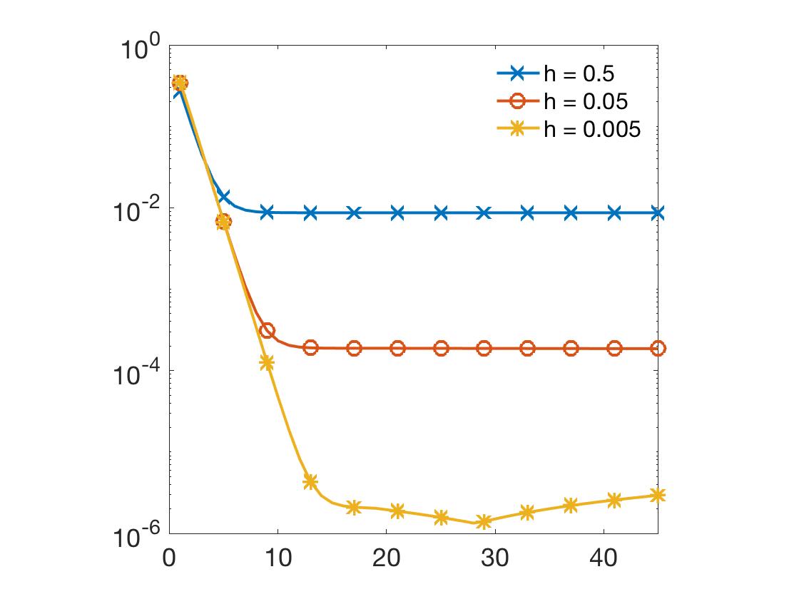
Fig. 4 shows the $L^{\infty}$ error between the numerical solution and the true solution for the different boundary conditions. Fig. 4(a) shows the whole real line numerical scheme where we’ve used the asymptotic decay rate of $\frac{1}{x^{2}}$ outside of $(-L,L)$ . Fig. 4(b) corresponds to the Dirichlet problem with homogeneous boundary conditions: $g(x)=0$ outside $(-L,L)$ . Finally, Fig. 4(c) corresponds to the Neumann problem with homogeneous boundary conditions: $g(x)=0$ outside $(-L,L)$ . To be clear, we’re setting up the Neumann problem on a uniform grid in $(-2L,2L)$ so that in order to use the previous numerical scheme we have to select $L_{W}\geq 4L$ . Although this requires roughly twice the computational cost of the other two methods it nevertheless compares the effectiveness of the boundary conditions. As the solution $u(x)$ decays exponentially, we note that enforcing homogeneous boundaries condition is consistent with the original problem when $L$ is large enough. With this in mind, it’s clear that for large enough $L$ any of the three schemes retains the $O(h^{2})$ converge rate.

As shown in Fig. 4(c) , the Neumann formulation requires larger value of $L$ to obtain a similar convergence behavior than the other formulations. It is a consequence of $\bar{f}$ being discontinuous even for large value of $L$ . However the Neumann formulation is still expected to converge with a $O(h^{2})$ rate as the function $\bar{f}$ will appear continuous to machine precision when $L$ is large enough.

In the second case we take

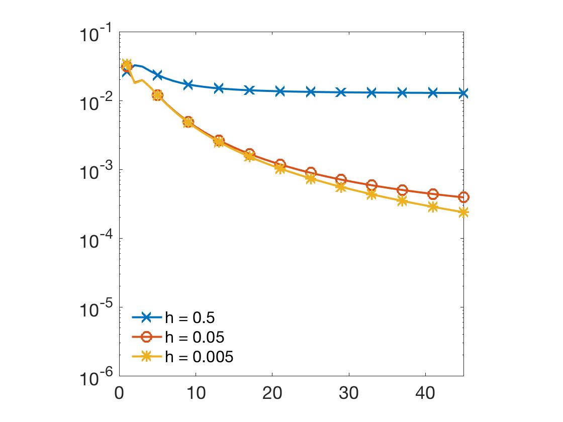
f(x)=\frac{1}{1+x^{2}}-\frac{1}{2}\;\frac{1}{1+(x-a)^{2}}-\frac{1}{2}\;\frac{1}{1+(x+a)^{2}}

with $a=1$ for which we also know the solution. Fig. 5 is the companion figure to Fig. 4. Fig. 5(a) shows the whole real line numerical scheme where we’ve used the asymptotic decay rate of $\frac{1}{x^{2}}$ outside of $(-L,L)$ . Fig. 5(b) corresponds to the Dirichlet problem with homogeneous boundary conditions: $g(x)=0$ outside $(-L,L)$ . Finally, Fig. 5(c) corresponds to the Neumann problem with homogeneous boundary conditions, $g(x)=0$ outside $(-L,L)$ , and we computed this numerically in the same way as was described in the previous paragraph. As the use of exact solutions to set boundary conditions is not feasible and realistic for physical applications, we use homogeneous conditions for the Dirichlet and Neumann problems. It allows us to compare the behavior of the three schemes when the solutions is not exponentially decaying and that only its order of algebraic decay is known for large $x$ . Unlike the previous case the situation here is much different. Namely, the whole real line method is by far more accurate than either of the other two. For the Dirichlet condition it’s because of the slow algebraic decay of the solution; on the domains considered $u(x)$ does not fall below $10^{-4}$ , making this a lower bound on the error for any values of $h$ . For the Neumann problem it’s even worse because, in addition to the slow decay rate, we have a discontinuity which is detectable to machine precision for all values of $L$ considered. Hence, decreasing $h$ will not decrease the error because the discontinuity will not vanish.

6.5 Dirichlet Problem with Not Strictly Positive Kernel

Consider the Dirichlet problem

\begin{cases}\mathcal{L}\ast u(x)=f(x),&x\in(-L,L),\\ u(x)=\text{sech}(x),&x\in(-L,L)^{c},\end{cases}

(25)

with

	$\displaystyle\nu(y)$	$\displaystyle=\frac{3}{2}e^{-\|y\|}-2e^{-2\|y\|},$
	$\displaystyle f(x)$	$\displaystyle=4\,{{e}}^{-x}+\frac{1}{{\cosh}\left(x\right)}-\frac{3\,\ln\left({{e}}^{2\,x}+1\right)\,{{e}}^{-x}}{2}+2\,{{e}}^{x}\,\left(2\,{\tan^{-1}}\left({{e}}^{x}\right)\,{{e}}^{x}-\pi\,{{e}}^{x}+2\right)$
		$\displaystyle-4\,{\tan^{-1}}\left({{e}}^{x}\right)\,{{e}}^{-2\,x}+\frac{3\,{{e}}^{x}\,\left(2\,x-\ln\left({{e}}^{2\,x}+1\right)\right)}{2}.$

Then by direct calculation, we have that

	$\displaystyle f_{1}(h)=\frac{1}{h^{2}}\big[\frac{{{e}}^{-2\,h}\,\left(2\,h^{2}+2\,h+1\right)}{2}-\frac{3\,{{e}}^{-h}\,\left(h^{2}+2\,h+2\right)}{2}+\frac{5}{2}\big]=-\frac{1}{6}h+O(h^{2}),$
	$\displaystyle f_{2}(h)=-\frac{1}{6}h^{5}+O(h^{6})\quad,\quad f_{3}(h)=-\frac{1}{10}h^{5}+O(h^{6})\quad,\quad f_{4}(h)=\frac{1}{2}h^{2}+O(h^{3}).$

Hence, we should generically expect the scheme to converge at rate $O(h^{2})$ .

In this particular case, $\nu(y)$ has the antiderivatives

F(y)=\frac{3}{2}{e}^{-\left|y\right|}-\frac{1}{2}{{e}}^{-2\,\left|y\right|}\;\;,\;\;F^{\prime}(y)=-{\text{sign}}\left(y\right)\,\left(\frac{3}{2}\,{{e}}^{-\left|y\right|}-{{e}}^{-2\,\left|y\right|}\right)\;\;,\;\;F^{\prime\prime}(y)=\frac{3}{2}e^{-|y|}-2e^{-2|y|},

so that now all of the $w_{j}$ can be calculated. We also have that the integral $A$ can be directly computed and is given by

A=3e^{-2L_{W}}-2e^{-4L_{W}}.

The integral $B_{i}$ can also be calculated directly and is given by

	$\displaystyle B_{i}=$	$\displaystyle 4\,{{e}}^{-2\,x_{i}}\,{\tan^{-1}}\left({{e}}^{-L}\,{{e}}^{x_{i}}\right)-4\,{{e}}^{-L-x_{i}}+\frac{3\,{{e}}^{-x_{i}}\,\left(2\,x_{i}+\ln\left({{e}}^{-2\,L}+{{e}}^{-2\,x_{i}}\right)\right)}{2}$
		$\displaystyle-\frac{3\,{{e}}^{x_{i}}\,\left(2\,x_{i}-\ln\left({{e}}^{-2\,L}+{{e}}^{2\,x_{i}}\right)\right)}{2}-4\,{{e}}^{x_{i}}\,\left({{e}}^{-L}-{\tan^{-1}}\left({{e}}^{-L}\,{{e}}^{-x_{i}}\right)\,{{e}}^{x_{i}}\right).$

We then have all the necessary quantities to implement the numerical scheme for the Dirichlet problem. First note that the true solution of this problem is in fact $u(x)=\text{sech}(x)$ ; this can be confirmed by a straightforward integration. Fig. 6(a) shows a plot of the solution $u(x)$ and the forcing function $f(x)$ . Fig. 6(b) shows the $L^{\infty}$ error between the numerical solution and the true solution for varying values of $L$ and $h$ . We see that for fixed $L$ the scheme does indeed converge at an $O(h^{2})$ rate.

7 Conclusion

In this paper we consider integro-differential equations that model the evolution process of quantities that experience a nonlocal form of dispersion. In particular, we look at diffusion processes that are modeled using convolution kernels that do not have compact support and decay exponentially at infinity. We develop algorithms for finding the steady states of these systems.

In contrast to previous methods which assume local boundary data, our numerical method accounts for the correct nonlocal nature of the boundary conditions. We present three numerical schemes addressing the case of nonlocal Dirichlet boundary conditions (DP), Neumann boundary conditions (NP), and the whole real line problem (RP).

When the equation is posed on the whole real line, we show that a unique solution exist, provided the right hand side decays at least algebraically and has zero mean and first moment. More importantly, the result shows that there is a relation between the decay of the right hand side and the decay of the solution. This information is then used to approximate the solution outside the computational domain and thus develop a scheme for RP.

Since nonlocal Neumann boundary conditions require us to approximate the solution outside a bounded domain, the numerical schemes for NP and RP are almost identical. In both cases the scheme boils down to inverting a matrix equation. We are able to show using a Neumann series that this matrix is invertible provided the convolution kernel is nonnegative. This also proves the convergence of the scheme.

For the Dirichlet problem, we consider kernels that can take on negative values, but that have positive tails. We show, using the theory of Toeplitz matrices, that this is enough to prove the convergence of the our numerical scheme. This is an improvement over previous results which are based on maximum principles and therefore require nonnegative kernels with compact support.

Finally, for applications where the model equations are posed on the whole real line, there is always a question of what are the best boundary conditions one can use to approximate solutions. Here we present a numerical scheme that does not require explicit boundary conditions. However, we do find that in certain circumstances, mainly when the right hand side decays exponentially, the Dirichlet problem provides a more efficient method for approximating the whole real line problem. First, because one can reduce the size of the computational domain, and secondly one does not have to approximate the solution outside this domain, i.e. setting the solution to zero gives a good approximation.

Appendix A Nonlocal Flux, Gauss Theorem, and an Example

In this section we summarize results presented in [19, 20], which generalize the concept of flux to include short as well as long range movement of particles. Then, in Subsection A.3 we use a very general and well known population model as an example of how this generalized version of flux, together with conservation of mass, gives rise to equation (1). Similar derivations have been done in [5].

As already pointed out in the introduction variations of equation (1) have been introduced in other contexts. Here we restrict ourselves to the population model, since we believe it provides a simple example where one can apply the notion of nonlocal Neumann boundary conditions presented in [19, 20]. For more information about other nonlocal models, the review paper by Fife [27] provides a good starting point for the case.

A.1 Nonlocal Flux

To give an intuitive notion of what constitutes a nonlocal flux, we first recall the traditional definition of this term. In physical applications flux represents the rate of motion per unit area of a quantity $u$ (fluid, concentration, number of particles) across some boundary. Implicit in this definition is the assumption that the transport of this quantity happens at small scales. However, in certain applications transport can occur over long, as well as short, spatial scales. Consider for example an area of vegetation with seeds that can travel close to as well as far from their originating organisms thanks to wind currents. In this case flux is no longer proportional to a local quantity, like $u$ (transport equation) or the gradient of $u$ (diffusion equation), but instead should be expressed through a nonlocal operator.

We can make these ideas more precise by looking again at our vegetation example. For simplicity assume for now that we only have one organism at position $y$ , whose seeds are entering a field $\Omega$ . Suppose as well that we have a function $\phi(x,y,t)$ that tells us the proportion of seeds from position $y\notin\Omega$ that fall in location $x\in\Omega$ per unit time. Then the flow of seeds from $y$ into region $\Omega$ is given by the integral

\int_{\Omega}\phi(x,y,t)\;dx.

More generally, one can construct a function $\psi(x,y,t)$ such that

\int_{\Omega}\psi(x,y,t)\;dx,

represents a nonlocal flux density. Then, the expression

\int_{\Omega_{1}}\int_{\Omega_{2}}\psi(x,y,t)\;dx\;dy

gives us the net nonlocal flux from region $\Omega_{1}$ into region $\Omega_{2}$ . If this expression is positive then indeed we have net flux from $\Omega_{1}$ into $\Omega_{2}$ . On the other hand, if this quantity is negative, then the net flow occurs in the reverse direction.

For the above definition to be consistent with our intuition of how flux should behave, one imposes an action-reaction principle. Given two distinct domains $\Omega_{1}$ , $\Omega_{2}$ we would like for the nonlocal flux from $\Omega_{1}$ into $\Omega_{2}$ to be equal in magnitude, but of opposite sign, as the the nonlocal flux from $\Omega_{2}$ into $\Omega_{1}$ , i.e.

\int_{\Omega_{1}}\int_{\Omega_{2}}\psi(x,y,t)\;dx\;dy+\int_{\Omega_{2}}\int_{\Omega_{1}}\psi(y,x,t)\;dy\;dx=0.

It is straightforward to check that this holds provided $\psi$ is antisymmetric in $x$ and $y$ , that is $\psi(x,y,t)=-\psi(y,x,t)$ . Notice that this condition also implies that there are no self interactions, meaning that

\int_{\Omega}\int_{\Omega}\psi(x,y,t)\;dx\;dy=0.

A.2 Nonlocal Gauss’ Theorem

Given a bounded domain $\Omega$ , Gauss’ Theorem relates the total flux across the boundary $\partial\Omega$ , in terms of a volume integral over the domain, $\Omega$ . More precisely, if ${\bf F}$ represents a smooth vector field and ${\bf n}$ the unit normal to $\Omega$ , then

\int_{\Omega}\nabla\cdot{\bf F}\;dV=\int_{\partial\Omega}{\bf F\cdot n}\;dS.

In the nonlocal case, the action-reaction principle provides an analogue to Gauss’ Theorem since it relates the flux from $\Omega^{c}$ into $\Omega$ in terms of an integral over $\Omega$ ,

\int_{\Omega^{c}}\int_{\Omega}\psi(x,y,t)\;dx\;dy=\int_{\Omega}\int_{\Omega^{c}}-\psi(x,y,t)\;dx\;dy.

A.3 Derivation equation with population dynamics example

To illustrate our point suppose we are interested in the evolution of a population that is able to move short as well as long distances. Let $u(x,t)$ denote the density of this population at time $t$ and location $x$ , and let $\Omega\subset\mathbb{R}^{n}$ be a bounded domain. Then $m=\int_{\Omega}u(x,t)\;dx$ represents the total number of individuals in $\Omega$ at time $t$ .

Assume as well that the fraction of the population that flows from $x$ to $y$ depends on the distance between these two points and is proportional to the density at point $x$ . More precisely, at time $t$ the flow from $x\in\Omega$ to $y\in\Omega^{c}$ is is given by the product $u(x,t)\nu(x,y)$ , where we also assume that the kernel $\nu(x,y)=\nu(|x-y|)$ is symmetric and exponentially decaying. Then, the flow from the point $x\in\Omega$ to the domain $\Omega^{c}$ is given by the integral

\int_{\Omega^{c}}u(x,t)\nu(|x-y|)\;dy,

and the total flow out of $\Omega$ can be represented by the expression

\int_{\Omega}\int_{\Omega^{c}}u(x,t)\nu(|x-y|)\;dy\;dx.

Similarly, the flow from $\Omega^{c}$ into the point $x\in\Omega$ can be written as

\int_{\Omega^{c}}u(y,t)\nu(|x-y|)\;dy

so that the total flow into $\Omega$ is

\int_{\Omega}\int_{\Omega^{c}}u(y,t)\nu(|x-y|)\;dy\;dx.

Combining these two expressions we find that the net flow, $Q$ , of the population in/out of the domain $\Omega$ is given by

	$\displaystyle Q=$	$\displaystyle-\int_{\Omega}\int_{\Omega^{c}}u(x,t)\nu(\|x-y\|)\;dy\;dx+\int_{\Omega}\int_{\Omega^{c}}u(y,t)\nu(\|x-y\|)\;dy\;dx$
	$\displaystyle Q=$	$\displaystyle\int_{\Omega}\int_{\Omega^{c}}-(u(x,t)-u(y,t))\nu(\|x-y\|)\;dy\;dx.$
	$\displaystyle Q=$	$\displaystyle\int_{\Omega}\int_{\mathbb{R}^{n}}\underbrace{-(u(x,t)-u(y,t))\nu(\|x-y\|)}_{=\psi(x,y,t)}\;dy\;dx.$

where the last line follows from the flow density function $\psi(x,y,t)$ being antisymmetric, and the fact that this rules out self-interactions.

By conservation of mass

m_{t}=\int_{\Omega}u_{t}\;dx=\int_{\Omega}\int_{\mathbb{R}^{n}}-(u(x,t)-u(y,t))\nu(|x-y|)\;dy\;dx+\int_{\Omega}f\;dx,

where $f(x)$ is a density specifying the net loss/gain of individuals at location $x$ that combines births and deaths. Since the domain $\Omega$ is arbitrary, the result is an evolution equation for the variable $u$ ,

u_{t}=-\mathcal{L}\ast u+f(x)\quad\mbox{for}\quad x\in\Omega

(26)

where

\mathcal{L}\ast u=\int_{\mathbb{R}^{n}}(u(x,t)-u(y,t))\nu(|x-y|)\;dy.

Now, because the flow is nonlocal, instead of boundary conditions across $\partial\Omega$ , we need to impose conditions on $\Omega^{c}$ :

•

Dirichlet: One specifies the value of the function $u$ in $\Omega^{c}$

$u(x)=g(x)\quad\mbox{for}\quad x\in\Omega^{c}.$
•

Neumann: Since by the nonlocal Gauss’ Theorem $\int_{\Omega^{c}}\int_{\mathbb{R}^{n}}-\psi(x,y,t)\;dy\;dx$ represents the net flow in/out of $\Omega^{c}$ , then the following relation specifies a given and fixed flow density, $f_{c}(x)$ , from $\Omega^{c}$ into the domain $\Omega$ ,

$\int_{\mathbb{R}^{n}}\psi(x,y,t)\;dy=f_{c}(x)\quad x\in\Omega^{c}.$

•

Mixed: Given $\Omega^{c}=\Omega^{c}_{1}\cup\Omega^{c}_{2}$

	$\displaystyle u(x)=g(x)$	$\displaystyle\quad\mbox{for}\quad x\in\Omega^{c}_{1},$
	$\displaystyle\int_{\mathbb{R}^{n}}\psi(x,y,t)\;dy=f_{c}(x)$	$\displaystyle\quad\mbox{for}\quad x\in\Omega^{c}_{2}.$

Appendix B Nonlocal Diffusive Operators on a Lattice

Here we extend the results of 3.1 to operators defined on lattices using results presented in [31].

We first define the analogue of the spaces $L^{2}_{\gamma}(\mathbb{R}),M^{2,s}_{\gamma}(\mathbb{R}),$ and $H^{s}_{\gamma}(\mathbb{R})$ in the obvious way and denote them by $\ell_{\gamma}^{2}(\mathbb{Z})$ , $m_{\gamma}^{2,s}(\mathbb{Z})$ , $h^{s}_{\gamma}(\mathbb{Z})$ , respectively. As above we use $\langle,\rangle$ to denote the pairing between dual elements, and we let $\underline{u}=\{u_{j}\}_{j\in\mathbb{Z}}$ . In the case of lattices, the Fourier Transform is given by

\begin{array}[]{c c c c}\mathcal{F}_{d}:&\ell^{2}(\mathbb{Z})&\longrightarrow&L^{2}(\mathbb{T}_{1})\\ &u=\{u_{j}\}_{j\in\mathbb{Z}}&\longmapsto&\hat{u}(\sigma)=\sum_{j\in\mathbb{Z}}u_{j}\mathrm{e}^{-2\pi\mathrm{i}j\sigma}\end{array}

where $\mathbb{T}_{1}=\mathbb{R}/\mathbb{Z}$ is the unit circle. We can also define discrete derivatives for elements in $\ell^{2}(\mathbb{Z}),$

\delta_{+}(\{u_{j}\}_{j\in\mathbb{Z}})=\{u_{j+1}-u_{j}\}_{j\in\mathbb{Z}}\qquad\delta_{-}(\{u_{j}\}_{j\in\mathbb{Z}})=\{u_{j}-u_{j-1}\}_{j\in\mathbb{Z}}\qquad\delta=-\mathrm{i}(\delta_{+}+\delta_{-})/2

with their corresponding Fourier symbols,

D_{+}(\sigma)=\mathrm{e}^{2\pi\mathrm{i}\sigma}-1,\quad D_{-}(\sigma)=1-\mathrm{e}^{-2\pi\mathrm{i}\sigma},\quad D(\sigma)=\sin(2\pi\sigma).

As was the case for operators defined on $L^{2}(\mathbb{R})$ , the Fourier Transform of general convolution operators, $L(\sigma)$ , is a multiplication symbol defined on the space $L^{2}(\mathbb{T}_{1})$ :

\begin{array}[]{c c c c}\hat{\mathcal{L}}:&D(\hat{\mathcal{L}})\subset L^{2}(\mathbb{T}_{1})&\longrightarrow&L^{2}(\mathbb{T}_{1})\\ &u(\sigma)&\longmapsto&L(\sigma)u(\sigma)\end{array}

Here, we make the following assumptions on the Fourier symbol $L(\sigma)$ , of our discrete convolution operators $\mathcal{L}$ .

Hypothesis B.1.

The symbol $L(\sigma)$ is analytic, uniformly bounded, and 1-periodic in a strip $\Omega_{1}=\mathbb{R}\times(\mathrm{i}\sigma_{1},\mathrm{i}\sigma_{1})$ for some $\sigma_{1}>0$ . Moreover, when restricted to $\sigma\in[-1/2,1/2]$ the symbol $L(\sigma)$ is invertible except at $\sigma=0$ , where it has a zero of multiplicity $m$ .

As was the case in the real line, the operator $\mathcal{L}$ can be decomposed into an invertible operator $\mathcal{M}_{L}(\sigma)$ and a Fredholm operator with Fourier symbol $(\mathrm{e}^{2\pi\mathrm{i}\sigma}-1)^{m}[1+\mathrm{i}C\sin^{l}(2\pi\sigma)]^{-1}$ , which formally corresponds to $\delta_{+}^{m}(1+\delta^{l})^{-1}$ . This leads to the following proposition.

Proposition B.2.

For $\gamma\notin\{1/2,3/2,\cdots,m-1/2\}$ , and appropriate value of the integer $l$ , the operator $\mathcal{L}:m^{2,m}_{\gamma}(\mathbb{Z})\longrightarrow h^{l}_{\gamma+m}(\mathbb{Z})$ satisfying Hypothesis B.1 is Fredholm. Moreover, letting $\underline{\eta}^{b}=\{\eta^{b}\}_{\eta\in\mathbb{Z}}$ , we have that

•

for $\gamma>-1/2$ the operator is injective with cokernel

$\mathop{\mathrm{Coker}\,}=\mathrm{span}\{\underline{\eta}^{\beta}\mid\beta=0,1,\cdots,m-1\}$
•

for $\gamma<1/2-m$ the operator is surjective with kernel

$\mathrm{Ker}\,=\mathrm{span}\{\underline{\eta}^{\beta}\mid\beta=0,1,\cdots,m-1\}$
•

for $j-1/2-m<\gamma<j-m+1/2$ , with $j\in\mathbb{Z}$ , $1\leq j<m$ , the operator has kernel

$\mathrm{Ker}\,=\mathrm{span}\{\underline{\eta}^{\beta}\mid\beta=0,1,\cdots,m-j-1\}$

and cokernel

$\mathop{\mathrm{Coker}\,}=\mathrm{span}\{\underline{\eta}^{\beta}\mid\beta=0,1,\cdots,j-1\}.$

On the other hand, the operator does not have closed range when $\gamma\in\{1/2,3/2,\cdots,m-1/2\}$ .

From the above result we obtain the next corollary, which we will use in the proof of convergence for the numerical schemes. In particular, the following result gives us information about the decay rate of solutions to the discrete convolution problem defined over $\ell^{2}(\mathbb{Z})$

\mathcal{L}\ast\underline{u}=\underline{f}.

Corollary B.3.

Consider the discrete convolution operator $\mathcal{L}$ , with Fourier symbol $(\mathrm{e}^{2\pi\mathrm{i}\sigma}-1)^{2}[1+(2\mathrm{i}\sin(2\pi\sigma)^{2}]^{-1}$ , and defined as

\begin{array}[]{c c c}\mathscr{L}:m^{2,2}_{\gamma}(\mathbb{Z})&\longrightarrow&h^{2}_{\gamma+2}(\mathbb{Z})\\ \underline{u}&\longmapsto&\mathcal{L}\ast\underline{u}.\end{array}

Suppose $\gamma>-1/2$ , then the equation $\mathcal{L}\ast\underline{u}=\underline{f}$ has a unique solution, with $|u_{j}|<C|j|^{1/2-(\gamma+1)}$ for large $|j|$ , provided the right hand side $\underline{f}\in h^{2}(\mathbb{Z})_{\gamma+2}$ satisfies

\langle\underline{f},\underline{1}\rangle=0\qquad\mbox{and}\qquad\langle\underline{f},\underline{\eta}\rangle=0.

Appendix C Calculation of $w_{j}$

Here we derive formulas for the weights $w_{j}$ considered earlier. Assume that $\nu(y)$ has two integrable antiderivatives. Namely, assume there exists a function $F$ such that $F^{\prime\prime}(y)=\nu(y)$ . We can then use integration by parts to show the following results.

In the first case, assume $1<|j|<M$ , then

	$\displaystyle\int_{h\leq\|y\|\leq L_{W}}T(y-x_{j})\nu(y)\;dy$	$\displaystyle=\int^{x_{j+1}}_{x_{j-1}}T(y-x_{j})\nu(y)\;dy$
		$\displaystyle=\int^{h}_{-h}T(z)\nu(z+x_{j})\;dz$
		$\displaystyle=\frac{1}{h}\bigg[F(x_{j+1})-2F(x_{j})+F(x_{j-1})\bigg].$

The second line is obtained by the change of variables $z=y-x_{j}$ . The third line is obtained by doing integration by parts twice and using $\nu=F^{{}^{\prime\prime}}$ .

When $j=1$ , we don’t integrate over the full hat function because half of the hat function is not in the domain of $|y|\geq h$ . It reads:

	$\displaystyle\int_{h\leq\|y\|\leq L_{W}}T(y-x_{1})\nu(y)\;dy$	$\displaystyle=\int^{x_{2}}_{x_{1}}T(y-x_{1})\nu(y)\;dy$
		$\displaystyle=\int^{h}_{0}T(z)\nu(z+x_{1})\;dz$
		$\displaystyle=\-F^{\prime}(x_{1})+\frac{1}{h}\bigg[F(x_{2})-F(x_{1})\bigg].$

When $j=M$ a similar argument shows

\int_{h\leq|y|\leq L_{W}}T(y-x_{M})\nu(y)\;dy=F^{\prime}(x_{M})+\frac{1}{h}[F(x_{M-1})-F(x_{M})].

Finally, because both $\nu(y)$ and $T(y)$ are even we have

	$\displaystyle\int_{h\leq\|y\|\leq L_{W}}T(y-x_{-j})\nu(y)\;dy$	$\displaystyle=\int_{h\leq\|y\|\leq L_{W}}T(y+x_{j})\nu(y)\;dy$
		$\displaystyle=\int_{h\leq\|z\|\leq L_{W}}T(-z+x_{j})\nu(-z)\;dz$
		$\displaystyle=\int_{h\leq\|z\|\leq L_{W}}T(z-x_{j})\nu(z)\;dz.$

Looking at the definitions in the previous sections, this immediately gives

w_{-j}=w_{j}.

To summarize, we’ve shown that if the kernel $\nu$ has the appropriate antiderivatives $F$ then the weights $w_{j}$ are given explicitly by

w_{j}=\begin{cases}f_{1}(h)-F^{\prime}(x_{1})+\frac{1}{h}[F(x_{2})-F(x_{1})],&|j|=1\\[5.69046pt] \frac{1}{h}[F(x_{j+1})-2F(x_{j})+F(x_{j-1})],&1<|j|<M\\[5.69046pt] F^{\prime}(x_{M})+\frac{1}{h}[F(x_{M-1})-F(x_{M})],&|j|=M\end{cases}

with $w_{0}=0$ .

References

[1] G. Acosta, F. M. Bersetche, and J. P. Borthagaray, A short FE implementation for a 2d homogeneous dirichlet problem of a fractional Laplacian, Computers & Mathematics with Applications, 74 (2017), pp. 784 – 816, https://doi.org/https://doi.org/10.1016/j.camwa.2017.05.026, http://www.sciencedirect.com/science/article/pii/S0898122117303310.
[2] G. Acosta and J. P. Borthagaray, A fractional Laplace equation: Regularity of solutions and finite element approximations, SIAM Journal on Numerical Analysis, 55 (2017), pp. 472–495, https://doi.org/10.1137/15M1033952, https://doi.org/10.1137/15M1033952, https://arxiv.org/abs/https://doi.org/10.1137/15M1033952.
[3] G. Alberti and G. Bellettini, A nonlocal anisotropic model for phase transitions, Mathematische Annalen, 310 (1998), pp. 527–560, https://doi.org/10.1007/s002080050159, https://doi.org/10.1007/s002080050159.
[4] S.-i. Amari, Dynamics of pattern formation in lateral-inhibition type neural fields, Biological Cybernetics, 27 (1977), pp. 77–87, https://doi.org/10.1007/BF00337259, https://doi.org/10.1007/BF00337259.
[5] F. Andreu-Vaillo, J. J. Toledo-Melero, J. M. Mazon, and J. D. Rossi, Nonlocal diffusion problems, no. 165, American Mathematical Soc., 2010.
[6] E. Askari, F. Bobaru, R. B. Lehoucq, M. L. Parks, S. A. Silling, and O. Weckner, Peridynamics for multiscale materials modeling, Journal of Physics: Conference Series, 125 (2008), p. 012078, https://doi.org/10.1088/1742-6596/125/1/012078, https://doi.org/10.1088%2F1742-6596%2F125%2F1%2F012078.
[7] M. Banerjee and V. Volpert, Spatio–temporal pattern formation in Rosenzweig–Macarthur model: Effect of nonlocal interactions, Ecological Complexity, 30 (2017), pp. 2 – 10, https://doi.org/https://doi.org/10.1016/j.ecocom.2016.12.002, http://www.sciencedirect.com/science/article/pii/S1476945X16301076. Dynamical Systems In Biomathematics.
[8] P. Bates, X. Chen, A. J. J. Chmaj, J. Han, C. Zhang, and G. Zhao, On some nonlocal evolution equations arising in materials science, 2008.
[9] P. W. Bates, P. C. Fife, X. Ren, and X. Wang, Traveling waves in a convolution model for phase transitions, Archive for Rational Mechanics and Analysis, 138 (1997), pp. 105–136, https://doi.org/10.1007/s002050050037, https://doi.org/10.1007/s002050050037.
[10] F. Bobaru, J. T. Foster, P. H. Geubelle, and S. A. Silling, Handbook of peridynamic modeling, CRC press, 2016.
[11] M. Bodnar and J. Velazquez, An integro-differential equation arising as a limit of individual cell-based models, Journal of Differential Equations, 222 (2006), pp. 341 – 380, https://doi.org/https://doi.org/10.1016/j.jde.2005.07.025, http://www.sciencedirect.com/science/article/pii/S0022039605002494.
[12] P. C. Bressloff, Spatiotemporal dynamics of continuum neural fields, Journal of Physics A: Mathematical and Theoretical, 45 (2011), p. 033001, https://doi.org/10.1088/1751-8113/45/3/033001, https://doi.org/10.1088%2F1751-8113%2F45%2F3%2F033001.
[13] C. Carrillo and P. Fife, Spatial effects in discrete generation population models, Journal of Mathematical Biology, 50 (2005), pp. 161–188, https://doi.org/10.1007/s00285-004-0284-4, https://doi.org/10.1007/s00285-004-0284-4.
[14] X. Chen and M. Gunzburger, Continuous and discontinuous finite element methods for a peridynamics model of mechanics, Computer Methods in Applied Mechanics and Engineering, 200 (2011), pp. 1237 – 1250, https://doi.org/https://doi.org/10.1016/j.cma.2010.10.014, http://www.sciencedirect.com/science/article/pii/S0045782510002926.
[15] S. Coombes, P. beim Graben, R. Potthast, and J. Wright, Neural fields: theory and applications, Springer, 2014, https://doi.org/10.1007/978-3-642-54593-1, https://doi.org/10.1007/978-3-642-54593-1.
[16] A. S. Dagbovie and J. A. Sherratt, Absolute stability and dynamical stabilisation in predator-prey systems, Journal of Mathematical Biology, 68 (2014), pp. 1403–1421, https://doi.org/10.1007/s00285-013-0672-8, https://doi.org/10.1007/s00285-013-0672-8.
[17] A. De Masi, T. Gobron, and E. Presutti, Travelling fronts in non-local evolution equations, Archive for Rational Mechanics and Analysis, 132 (1995), pp. 143–205, https://doi.org/10.1007/BF00380506, https://doi.org/10.1007/BF00380506.
[18] M. D’Elia, M. D. Gunzburger, and C. Vollmann, A cookbook for finite element methods for nonlocal problems including quadrature rule choices and the use of approximate balls., tech. report, Sandia National Lab.(SNL-NM), Albuquerque, NM (United States), 2020.
[19] Q. Du, M. Gunzburger, R. B. Lehoucq, and K. Zhou, Analysis and approximation of nonlocal diffusion problems with volume constraints, SIAM Review, 54 (2012), pp. 667–696, https://doi.org/10.1137/110833294, https://doi.org/10.1137/110833294, https://arxiv.org/abs/https://doi.org/10.1137/110833294.
[20] Q. Du, M. Gunzburger, R. B. Lehoucq, and K. Zhou, A nonlocal vector calculus, nonlocal volume-constrained problems, and nonlocal balance laws, Mathematical Models and Methods in Applied Sciences, 23 (2013), pp. 493–540, https://doi.org/10.1142/S0218202512500546, https://doi.org/10.1142/S0218202512500546, https://arxiv.org/abs/https://doi.org/10.1142/S0218202512500546.
[21] S. Duo, H. W. van Wyk, and Y. Zhang, A novel and accurate finite difference method for the fractional Laplacian and the fractional Poisson problem, Journal of Computational Physics, 355 (2018), pp. 233 – 252, https://doi.org/https://doi.org/10.1016/j.jcp.2017.11.011, http://www.sciencedirect.com/science/article/pii/S0021999117308495.
[22] S. Duo and Y. Zhang, Accurate numerical methods for two and three dimensional integral fractional Laplacian with applications, Computer Methods in Applied Mechanics and Engineering, 355 (2019), pp. 639 – 662, https://doi.org/https://doi.org/10.1016/j.cma.2019.06.016, http://www.sciencedirect.com/science/article/pii/S0045782519303597.
[23] M. D’Elia and M. Gunzburger, The fractional Laplacian operator on bounded domains as a special case of the nonlocal diffusion operator, Computers & Mathematics with Applications, 66 (2013), pp. 1245 – 1260, https://doi.org/https://doi.org/10.1016/j.camwa.2013.07.022, http://www.sciencedirect.com/science/article/pii/S0898122113004707.
[24] L. Eigentler and J. A. Sherratt, Analysis of a model for banded vegetation patterns in semi-arid environments with nonlocal dispersal, Journal of Mathematical Biology, 77 (2018), pp. 739–763, https://doi.org/10.1007/s00285-018-1233-y, https://doi.org/10.1007/s00285-018-1233-y.
[25] G. B. Ermentrout and J. D. Cowan, A mathematical theory of visual hallucination patterns, Biological Cybernetics, 34 (1979), pp. 137–150, https://doi.org/10.1007/BF00336965, https://doi.org/10.1007/BF00336965.
[26] P. J. S. Ferreira, Localization of the eigenvalues of toeplitz matrices using additive decomposition, embedding in circulants, and the fourier transform, IFAC Proceedings Volumes, 27 (1994), pp. 1227 – 1232, https://doi.org/https://doi.org/10.1016/S1474-6670(17)47877-3, http://www.sciencedirect.com/science/article/pii/S1474667017478773. IFAC Symposium on System Identification (SYSID’94), Copenhagen, Denmark, 4-6 July.
[27] P. Fife, Some nonclassical trends in parabolic and parabolic-like evolutions, in Trends in Nonlinear Analysis, M. Kirkilionis, S. Krömker, R. Rannacher, and F. Tomi, eds., Berlin, Heidelberg, 2003, Springer Berlin Heidelberg, pp. 153–191.
[28] V. García-Morales and K. Krischer, Nonlocal complex Ginzburg–Landau equation for electrochemical systems, Phys. Rev. Lett., 100 (2008), p. 054101, https://doi.org/10.1103/PhysRevLett.100.054101, https://link.aps.org/doi/10.1103/PhysRevLett.100.054101.
[29] Genieys, S., Volpert, V., and Auger, P., Pattern and waves for a model in population dynamics with nonlocal consumption of resources, Math. Model. Nat. Phenom., 1 (2006), pp. 63–80, https://doi.org/10.1051/mmnp:2006004, https://doi.org/10.1051/mmnp:2006004.
[30] Y. Huang and A. Oberman, Numerical methods for the fractional Laplacian: A finite difference-quadrature approach, SIAM Journal on Numerical Analysis, 52 (2014), pp. 3056–3084, https://doi.org/10.1137/140954040, https://doi.org/10.1137/140954040, https://arxiv.org/abs/https://doi.org/10.1137/140954040.
[31] G. Jaramillo, A. Scheel, and Q. Wu, The effect of impurities on striped phases, Proceedings of the Royal Society of Edinburgh: Section A Mathematics, 149 (2019), pp. 131– 168, https://doi.org/10.1017/S0308210518000197.
[32] G. Jaramillo and S. C. Venkataramani, Target patterns in a 2d array of oscillators with nonlocal coupling, Nonlinearity, 31 (2018), pp. 4162–4201, https://doi.org/10.1088/1361-6544/aac9a6, https://doi.org/10.1088%2F1361-6544%2Faac9a6.
[33] A.-K. Kassam and L. N. Trefethen, Fourth-order time-stepping for stiff pdes, SIAM Journal on Scientific Computing, 26 (2005), pp. 1214–1233, https://doi.org/10.1137/S1064827502410633, https://doi.org/10.1137/S1064827502410633, https://arxiv.org/abs/https://doi.org/10.1137/S1064827502410633.
[34] M. Kot, M. A. Lewis, and P. van den Driessche, Dispersal data and the spread of invading organisms, Ecology, 77 (1996), pp. 2027–2042, https://doi.org/10.2307/2265698, https://esajournals.onlinelibrary.wiley.com/doi/abs/10.2307/2265698, https://arxiv.org/abs/https://esajournals.onlinelibrary.wiley.com/doi/pdf/10.2307/2265698.
[35] C. R. Laing, Spiral waves in nonlocal equations, SIAM Journal on Applied Dynamical Systems, 4 (2005), pp. 588–606, https://doi.org/10.1137/040612890, https://doi.org/10.1137/040612890, https://arxiv.org/abs/https://doi.org/10.1137/040612890.
[36] E. Madenci and E. Oterkus, Peridynamic Theory and Its Applications, Springer, 2014, https://doi.org/10.1007/978-1-4614-8465-3.
[37] A. D. Masi, E. Orlandi, E. Presutti, and L. Triolo, Glauber evolution with kac potentials. i. mesoscopic and macroscopic limits, interface dynamics, Nonlinearity, 7 (1994), pp. 633–696, https://doi.org/10.1088/0951-7715/7/3/001, https://doi.org/10.1088%2F0951-7715%2F7%2F3%2F001.
[38] D. Mollison, Spatial contact models for ecological and epidemic spread, Journal of the Royal Statistical Society: Series B (Methodological), 39 (1977), pp. 283–313, https://doi.org/10.1111/j.2517-6161.1977.tb01627.x, https://rss.onlinelibrary.wiley.com/doi/abs/10.1111/j.2517-6161.1977.tb01627.x, https://arxiv.org/abs/https://rss.onlinelibrary.wiley.com/doi/pdf/10.1111/j.2517-6161.1977.tb01627.x.
[39] S.-i. Shima and Y. Kuramoto, Rotating spiral waves with phase-randomized core in nonlocally coupled oscillators, Phys. Rev. E, 69 (2004), p. 036213, https://doi.org/10.1103/PhysRevE.69.036213, https://link.aps.org/doi/10.1103/PhysRevE.69.036213.
[40] J. Siebert, S. Alonso, M. Bär, and E. Schöll, Dynamics of reaction–diffusion patterns controlled by asymmetric nonlocal coupling as a limiting case of differential advection, Phys. Rev. E, 89 (2014), p. 052909, https://doi.org/10.1103/PhysRevE.89.052909, https://link.aps.org/doi/10.1103/PhysRevE.89.052909.
[41] S. Silling, Reformulation of elasticity theory for discontinuities and long-range forces, Journal of the Mechanics and Physics of Solids, 48 (2000), pp. 175 – 209, https://doi.org/https://doi.org/10.1016/S0022-5096(99)00029-0, http://www.sciencedirect.com/science/article/pii/S0022509699000290.
[42] S. Silling and R. Lehoucq, Peridynamic theory of solid mechanics, in Advances in Applied Mechanics, H. Aref and E. van der Giessen, eds., vol. 44 of Advances in Applied Mechanics, Elsevier, 2010, pp. 73 – 168, https://doi.org/https://doi.org/10.1016/S0065-2156(10)44002-8, http://www.sciencedirect.com/science/article/pii/S0065215610440028.
[43] S. A. Silling and R. B. Lehoucq, Convergence of peridynamics to classical elasticity theory, Journal of Elasticity, 93 (2008), pp. 13–37, https://doi.org/10.1007/s10659-008-9163-3.
[44] S. A. Silling, M. Zimmermann, and R. Abeyaratne, Deformation of a peridynamic bar, Journal of Elasticity, 73 (2003), pp. 173–190, https://doi.org/10.1023/B:ELAS.0000029931.03844.4f, https://doi.org/10.1023/B:ELAS.0000029931.03844.4f.
[45] D. Tanaka and Y. Kuramoto, Complex Ginzburg–Landau equation with nonlocal coupling, Phys. Rev. E, 68 (2003), p. 026219, https://doi.org/10.1103/PhysRevE.68.026219, https://link.aps.org/doi/10.1103/PhysRevE.68.026219.
[46] Y. Tao, X. Tian, and Q. Du, Nonlocal diffusion and peridynamic models with Neumann type constraints and their numerical approximations, Applied Mathematics and Computation, 305 (2017), pp. 282 – 298, https://doi.org/https://doi.org/10.1016/j.amc.2017.01.061, http://www.sciencedirect.com/science/article/pii/S0096300317300875.
[47] X. Tian and Q. Du, Analysis and comparison of different approximations to nonlocal diffusion and linear peridynamic equations, SIAM Journal on Numerical Analysis, 51 (2013), pp. 3458–3482, https://doi.org/10.1137/13091631X, https://doi.org/10.1137/13091631X, https://arxiv.org/abs/https://doi.org/10.1137/13091631X.
[48] O. Weckner, G. Brunk, M. A. Epton, S. A. Silling, and E. Askari, Green’s functions in non-local three-dimensional linear elasticity, Proceedings of the Royal Society A: Mathematical, Physical and Engineering Sciences, 465 (2009), pp. 3463–3487, https://doi.org/10.1098/rspa.2009.0234, https://royalsocietypublishing.org/doi/abs/10.1098/rspa.2009.0234, https://arxiv.org/abs/https://royalsocietypublishing.org/doi/pdf/10.1098/rspa.2009.0234.
[49] K. Zhou and Q. Du, Mathematical and numerical analysis of linear peridynamic models with nonlocal boundary conditions, SIAM Journal on Numerical Analysis, 48 (2010), pp. 1759–1780, https://doi.org/10.1137/090781267, https://doi.org/10.1137/090781267, https://arxiv.org/abs/https://doi.org/10.1137/090781267.

	$\displaystyle\\|E^{h}\\|_{2}$	$\displaystyle\leq\\|N^{-1}\\|_{2}\\|LTE\\|_{2}$
		$\displaystyle\leq\frac{1}{\Lambda_{\min}}\\|LTE\\|_{2}$
		$\displaystyle\leq\frac{\sqrt{L}}{\Lambda_{\min}}\\|LTE\\|_{\infty}$

	$\displaystyle A+c^{1}$	$\displaystyle=\int_{\|y\|\geq L_{W}}\nu(y)\;dy+\sum_{j=-M}^{M}w_{j}$
		$\displaystyle=\int_{\|y\|\geq L_{W}}\nu(y)\;dy+\sum_{j=-M}^{M}\int_{h\leq\|y\|\leq L_{W}}T(y-x_{j})\nu(y)\;dy+2f_{1}(h)$
		$\displaystyle=\int_{\|y\|\geq L_{W}}\nu(y)\;dy+\int_{h\leq\|y\|\leq L_{W}}\bigg(\sum_{j=-M}^{M}T(y-x_{j})\bigg)\nu(y)\;dy+2f_{1}(h)$
		$\displaystyle=\int_{\|y\|\geq L_{W}}\nu(y)\;dy+\int_{h\leq\|y\|\leq L_{W}}\nu(y)\;dy+2f_{1}(h)$
		$\displaystyle\leq 1,$

	$\displaystyle P_{k}(L)$	$\displaystyle=\int_{\|y\|\geq L_{W}}(1-\|L\|^{q}g(x_{-\frac{M}{2}+k}-y))\nu(y)\;dy$
		$\displaystyle=\int_{\|y\|\geq L_{W}}(1-\frac{\|L\|^{q}}{\|x_{-\frac{M}{2}+k}-y\|^{q}})\nu(y)\;dy$
		$\displaystyle\geq\int_{\|y\|\geq 2L_{W}}(1-\frac{\|L\|^{q}}{\|x_{-\frac{M}{2}+k}-y\|^{q}})\nu(y)\;dy$
		$\displaystyle\geq\int_{\|y\|\geq 2L_{W}}(1-\frac{\|L\|^{q}}{\|3L\|^{q}})\nu(y)\;dy$
		$\displaystyle=(1-\frac{1}{3^{q}})\int_{\|y\|\geq 2L_{W}}\nu(y)\;dy.$

	$\displaystyle\\|N^{-1}\\|_{\infty}$	$\displaystyle=\\|(I-Z)^{-1}\\|_{\infty}$
		$\displaystyle=\\|\sum_{n=0}^{\infty}Z^{n}\\|_{\infty}$
		$\displaystyle\leq\sum_{n=0}^{\infty}\\|Z\\|_{\infty}^{n}$
		$\displaystyle\leq\sum_{n=0}^{\infty}(1-\Lambda_{\min})^{n}$
		$\displaystyle=\frac{1}{\Lambda_{\min}}.$

	$\displaystyle\|u(x-y)-\frac{u(\pm L)}{g(\pm L)}g(x-y)\|$	$\displaystyle\leq\|u(x-y)\|+\|u(\pm L)\frac{g(x-y)}{g(\pm L)}\|$
		$\displaystyle\leq\frac{C}{\|x-y\|^{q}}+\frac{C}{\|L\|^{q}}\frac{\|L\|^{q}}{\|x-y\|^{q}}$
		$\displaystyle\leq\frac{2C}{\|x-y\|^{q}}$
		$\displaystyle\leq\frac{2C}{\|L\|^{q}}.$

Numerical Methods for a Diffusive Class Nonlocal Operators Thanks: This work is supported in part by the National Science Foundation under grant DMS-1911742 (GJ).

Abstract

keywords

AMS

1 Introduction

2 Nonlocal diffusion model and boundary conditions

Remark 2.1.

3 Weighted Spaces and Well-Posedness

3.1 Notation and Weighted Sobolev Spaces

Lemma 3.1.

Proof.

3.2 Nonlocal Diffusive Operators on the Real Line

Hypothesis 3.2.

Hypothesis 3.3.

Remark 3.4.

Remark 3.5.

Theorem 1.

Lemma 3.6.

Proposition 3.7.

Proposition 3.8.

Corollary 3.9.

Remark 3.10.

Remark 3.11.

Remark 3.12.

4 A Numerical Method for nonlocal diffusive operators

4.1 Discretization of the Operator

4.1.1 Discretization of the Singular Integral

4.1.2 Discretization of the Tail Integral

4.1.3 Discretization of the Nonlocal Operator

Remark 4.1.

4.2 Numerical Methods on a Finite Lattice

4.3 Dirichlet Problem

4.4 Whole Real Line Problem

4.5 Neumann Problem

5 Proofs of Convergence

5.1 Dirichlet

5.1.1 Stability

5.1.2 Consistency

5.1.3 Convergence

5.2 Whole Real Line Problem

5.2.1 Stability

5.2.2 Consistency

5.2.3 Convergence

6 Numerical illustrations

6.1 Dirichlet Problem

6.2 Whole Real Line Problem

6.3 Neumann Problem

6.4 Comparison of the Boundary Conditions

6.5 Dirichlet Problem with Not Strictly Positive Kernel

7 Conclusion

Appendix A Nonlocal Flux, Gauss Theorem, and an Example

A.1 Nonlocal Flux

A.2 Nonlocal Gauss’ Theorem

A.3 Derivation equation with population dynamics example

Appendix B Nonlocal Diffusive Operators on a Lattice

Hypothesis B.1.

Proposition B.2.

Corollary B.3.

Appendix C Calculation of wjw_{j}

References

Appendix C Calculation of $w_{j}$