Rotational modulation and single g-mode pulsation in the B9pSi star HD 174356?2020Rotational modulation and single g-mode pulsation in the B9pSi star HD 174356?–8
Abstract
Chemically peculiar (CP) stars of the upper main sequence are characterised by specific anomalies in the photospheric abundances of some chemical elements. The group of CP2 stars, which encompasses classical Ap and Bp stars, exhibits strictly periodic light, spectral, and spectropolarimetric variations that can be adequately explained by the model of a rigidly rotating star with persistent surface structures and a stable global magnetic field. Using observations from the Kepler K2 mission, we find that the B9pSi star HD 174356 displays a light curve both variable in amplitude and shape, which is not expected in a CP2 star. Employing archival and new photometric and spectroscopic observations, we carry out a detailed abundance analysis of HD 174356 and discuss its photometric and astrophysical properties in detail. We employ phenomenological modeling to decompose the light curve and the observed radial velocity variability. Our abundance analysis confirms that HD 174356 is a silicon-type CP2 star. No magnetic field stronger than 110 G was found. The star’s light curve can be interpreted as the sum of two independent strictly periodic signals with and . The periods have remained stable over 17 years of observations. In all spectra, HD 174356 appears to be single-lined. From the simulation of the variability characteristics and investigation of stars in the close angular vicinity, we put forth the hypothesis that the peculiar light variability of HD 174356 arises in a single star and is caused by rotational modulation due to surface abundance patches () and g mode pulsation ().
Keywords:
stars: chemically peculiar - variables: General - binaries: close - stars: individual: HD 1743561 Introduction
Chemically peculiar (CP) stars constitute about 10-15 % of the upper main-sequence stars between spectral types B2 and F5 (Preston 1974). They are characterised by abundance anomalies of individual chemical elements (typically Si, He, Fe, rare earths, Co, Ni, Ti, Sr, Sc, Ca, and others) in their outer layers that may reach several orders of magnitude as compared to the solar values. The observed peculiar abundances are generally explained by chemical segregation due to the interplay of radiative levitation and gravitational settling taking place in the calm radiative outer layers of mostly slowly rotating stars (Richer et al. 2000, e.g.).

Chemically peculiar stars are divided into several types according to their abundance patterns and effective temperatures. The group of CP2 stars, which encompasses classical Ap and Bp stars, has been well studied. Together with the He-weak and He-strong stars (also termed CP4/5 and CP6/7 stars; cf. Maitzen 1984), these objects are also referred to as magnetic chemically peculiar (mCP) stars because of the near-ubiquitous presence of a globally-organised magnetic field that may attain strengths of up to several tens of kG (Babcock 1958; Babcock 1960; Mathys 2001). We note, however, that the mCP classification might be occasionally misleading, as we know several well-studied CP2 stars with very weak (Shulyak et al. 2010, UMa;) or unmeasurable (Krtička et al. 2009, EE Dra;) magnetic fields.
Besides the detection of a magnetic field, there exist other indicators of mCP stars, such as the presence of strictly periodic spectral, photometric, and spectropolarimetric variability that is well described by the oblique rotator model (Stibbs 1950). The spectral changes indicate an uneven surface distribution of overabundant/underabundant chemical elements (abundance spots and patches) that persists for decades and more. The photometric variations, traditionally referred to as Canum Venaticorum (ACV) variability (Samus et al. 2017), are caused by the redistribution of flux in the abundance patches (Krtička et al. 2007; Krtička et al. 2013, e.g.), while the periodic spectropolarimetric changes are the result of rotation in the presence of a more or less dipole/quadrupole-like magnetic field that is frozen into the outer layers of the star. A direct link between magnetic field geometry and the location of the spectroscopic and photometric spots on mCP stars has not been proven (Jagelka et al. 2019). Nevertheless, we assume that, in addition to calm photospheres and slow rotation, global magnetic fields contribute to the stabilisation of the surface structures.
In the spectral realm of the mCP stars, we also encounter classical pulsators (Pigulski 2014a). Pulsating stars allow to probe stellar interiors that are not accessible to direct observations because the physical conditions and processes within a star significantly influence the observed pulsation periods and amplitudes. In this way, basic stellar properties such as mass, radius and distance can be derived (Belkacem et al. 2011; Aerts 2015).
2 HD 174356 – basic information
HD 174356 (CD 24 14762, TYC 6864-121-1) was identified as a standard CP2 star of type B9pSi in the past (Houk & Smith-Moore 1988; Renson & Manfroid 2009). However, the star was found to display a light curve both variable in amplitude and shape (see Fig. 1), which is not expected in a CP2 star.
The light variability of HD 174356 was first reported by Hümmerich et al. 2016, who listed a rotational period of 4.0431(3) d based on ASAS-3 photometry. Recently, Bowman et al. 2018 confirmed this period using Kepler K2 data. They furthermore detected a second period in the amplitude spectrum, which is not well-resolved from the harmonic of the measured rotation period. They suggested that HD 174356 may be a binary or multiple system and pointed out the similarity between its light curve and the light curves of cool differentially-rotating spotted stars. No further analysis of the variability characteristics was done in Bowman et al. 2018.
The Data Release 2 of the satellite mission (Gaia Collaboration et al. 2016; Gaia Collaboration et al. 2018; Lindegren et al. 2018)11 1 http://vizier.u-strasbg.fr/viz-bin/VizieR-3?-source=I/345/gaia2 lists a parallax of = 1.17(11) mas, which converts to a distance modulus mag. Employing the 3-D dust maps of the Pan-STARRS1 project (Green et al. 2015), we find that the star is located in a region of the Milky Way ( = 1093 and = 1079) significantly affected by interstellar extinction. For the above listed distance modulus, a reddening mag was deduced from the maps.
Adopting these values, the observed ( index of 0.21 mag, corrected for interstellar reddening of mag, locates the object in the region of the late B-type stars (Kharchenko 2001, 12 000 K,), which is consistent with the observed 2MASS (Skrutskie et al. 2006) photometry. Assuming (Majaess et al. 2016; Berdnikov et al. 1996; Pejcha & Kochanek 2012, e.g.), we estimate an apparent magnitude of mag and an absolute magnitude of mag, both corrected for dust extinction. These values also agree with the observed spectral type and the derived effective temperature.
In this paper, we study and discuss the photometric and spectroscopic properties of HD 174356, with the goal of revealing the cause of its unique light variability and the nature of the object(s) involved. To this end, we employ and analyse archival observations and own data of various kinds.
3 Observations
In the following sections, we provide information on the photometric and spectroscopic observations used in this study.
3.1 Photometry
Three different data sources and own observations were employed, which are described in more detail below. HD 174356 is not scheduled for any TESS observations.22 2 https://heasarc.gsfc.nasa.gov/cgi-bin/tess/webtess/wtv.py The characteristics of the employed photometric data are summarized in Table 1.
3.1.1 ASAS-3 observations
The All Sky Automated Survey (ASAS) monitored the southern and part of the northern sky (up to +28°), with the goal of investigating any kind of stellar photometric variability. Here we employ Johnson observations from the third phase of the project, ASAS-3, which were obtained with two wide-field telescopes equipped with f/2.8 200 mm Minolta lenses and AP 10 Apogee detectors (sky coverage ) located at the ten-inch astrograph dome of the Las Campanas Observatory in Chile. The typical exposure time was three minutes. The most reliable light curves were obtained for objects in the magnitude range 8 10 mag (typical scatter of about 0.01 mag; Pigulski 2014b). Frequency identification is rendered difficult because of strong daily aliases in the Fourier spectra based on ASAS-3 data. In this work, we employ only data points with quality flags “A” and “B”, which identify the most reliable data. Obvious outliers were removed by visual inspection.
| Source | Filter | Coverage | ||
| [mmag] | ||||
| ASAS-3 | 2001-2009 | 590 | 12 | |
| Kepler K2 | 2015-2016 | 3718 | 0.5 | |
| ASAS-SN | 2016-2018 | 433 | 23 |
3.1.2 Kepler K2 observations
The spacecraft boasts a differential photometer with 0.95 m aperture and detectors consisting of 21 modules each equipped with pixel CCD detectors. It produces ultra-precise single-passband (420-900 nm) light curves obtained in long-cadence (29.4 min) and short-cadence (58.5 s) modes. After the loss of two reaction wheels, the spacecraft was recommissioned to observe the ecliptic plane in the K2 mission (Howell et al. 2014). To adjust the pointing of the spacecraft, the on-board thrusters are fired at intervals of about six hours, which leads to characteristic systematics in the data sets (Howell et al. 2014).
About 3700 measurements in long-cadence mode were obtained of HD 174356 during a time span of 81.3 days (October 4 to December 26, 2015) in Campaign 7 of the K2 mission. The corresponding light curve was procured from the archive of K2 Data Products at the Mikulski Archive for Space Telescopes.33 3 https://archive.stsci.edu/k2/
The thruster firing signature at integers of 4.08 d-1 is obvious in the data. It is, however, of comparably low amplitude and does not interfere with the frequency analysis. We investigated the plots of Luger et al. 2016 to check for contamination of the light curve by neighbouring sources; no significant contaminating sources were identified.
3.1.3 ASAS-SN observations
All-Sky Automated Survey for Supernovae (ASAS-SN) observations are obtained at five stations, each of which is equipped with four 14 cm aperture Nikon telephoto lenses. Every clear night, the entire visible sky is observed to a depth of 17 mag in three dithered 90 s exposures made through or band filters (Shappee et al. 2014; Kochanek et al. 2017). The available data boast time baselines of up to five years. Depending on camera and image position, saturation issues set in at 10 to 11 mag. The effects of saturation are counterbalanced using a procedure inherited from the original ASAS survey, which is described in detail in Jayasinghe et al. 2018.
3.1.4 Own observations of HD 174356 and stars in its vicinity
We have carried out CCD photometric observations of HD 174356 and its vicinity using the STE4 camera attached to the 1 m telescope on the SAAO at Sutherland, South Africa (March 2018), and the 1.54 m Danish telescope at the La Silla Observatory in Chile (April 2018). At both sites, a Johnson filter was used. The seeing was between 0.8″ and 1.2″.
3.2 Spectroscopy and spectropolarimetry
To determine astrophysical parameters, investigate the presence of chemical peculiarities and magnetic field indicators, and look for possible signs of binarity, as suggested by Bowman et al. 2018, HD 174356 was investigated spectroscopically. Spectra from the following instruments were used:
- •
EBASIM Spectrograph at the 2.15m telescope at Complejo Astronómico El Leoncito (CASLEO, Argentina), 226 lines/mm grating, R 40 000, 4520 Å to 6520 Å, September 2018.
- •
Fiber-fed Extended Range Optical Spectrograph (FEROS) spectrograph attached to the 2.2m MPG/ESO telescope at La Silla Observatory (ESO) in Chile, , 3705 Å to 9225 Å, August 2017, Prog. ID: 099.A-9039(C).
- •
Goodman High Throughput Spectrograph (GTHS) at the 4.1m Southern Astrophysical Research (SOAR) telescope, red camera, 2100 lines/mm grating, R 11 000, 4460 Å to 5090 Å, September 2018, April 2019.
- •
High Accuracy Radial velocity Planet Searcher (HARPS) spectrograph at the ESO La Silla 3.6m telescope in Chile, R 110 000, 3900 Å to 6900 Å, June 2017, Prog. ID: 099.C-0081(A).
- •
HIgh-Dispersion Echelle Spectrograph (HIDES) at the 1.88m telescope of the Okayama Astrophysical Observatory (OAO) in Japan, R 50 000, 4090 Å to 7 520 Å, May 2017.
- •
Poznań Spectroscopic Telescope 2 (PST2) located at Winer Observatory in Arizona, R 40 000, 3890 Å to 9130 Å, March 2017.
Spectra were bias-corrected and flat-fielded, and data were reduced using standard IRAF routines.44 4 IRAF is distributed by NOAO, which is operated by AURA, Inc., under cooperative agreement with the National Science Foundation. A Th-Ar-Ne comparison spectrum was employed for precise wavelength calibration of the FEROS spectra, which was simultaneously obtained through a second fiber. In the case of the other instruments, we used Th-Ar spectra that were measured before and after the stellar spectrum.
The spectropolarimetric observations obtained with HARPSpol were reduced and calibrated with the HARPS data reduction software that is available at ESO. The normalization of the spectra to the continuum level was described in detail by Hubrig et al. 2013.
4 Analysis
4.1 Atmospheric parameters
Following Catanzaro et al. 2010, we determined effective temperature and surface gravity by comparing the observed and synthetic hydrogen H and H lines using the averaged FEROS spectrum, which does not suffer from normalization issues of the strongly broadened hydrogen lines. The corresponding uncertainties were calculated by taking into account the differences in the values obtained from the individual Balmer lines.
In a subsequent step, the and values obtained from the hydrogen-line fitting process were checked by analysis of the Fe i and Fe ii lines. We here used the high-resolution averaged HARPS spectrum and adjusted the effective temperature until no trend in the abundance versus excitation potential for the Fe ii lines remained. To determine , we relied on the ionization equilibrium of the Fe i and Fe ii lines. Furthermore, microturbulence was adjusted in such a way that trends of Fe ii abundance versus line strength were removed. Simultaneously, we obtained the projected rotational velocity . The employed spectrum synthesis method allows the simultaneous determination of various interlinked parameters such as , , , , and the relative abundances of the elements. Atmospheric parameters were obtained before the chemical abundance analysis.
We used one-dimensional plane-parallel hydrostatic models that assume radiative equilibrium and were calculated with the ATLAS 9 code (Kurucz 2014). Synthetic spectra were obtained using the line-blanketed local thermodynamical equilibrium code SYNTHE (Kurucz 2005). The codes were ported to GNU/Linux by Sbordone 2005. We made use of the most recent line list available at the Fiorella Castelli website.55 5 http://wwwuser.oats.inaf.it/castelli/
| Elem. | Abund. | SA | Elem. | Abund. | SA | ||
|---|---|---|---|---|---|---|---|
| He (2) | 4 | 10.19(20) | 10.93 | Ti (22) | 8 | 5.43(24) | 4.95 |
| C (6) | 4 | 8.69(25) | 8.43 | V (23) | 2 | 3.93(1) | 3.93 |
| N (7) | 2 | 7.31(1) | 7.83 | Cr (24) | 22 | 6.15(30) | 5.64 |
| O (8) | 4 | 8.59(25) | 8.69 | Mn (25) | 13 | 6.63(27) | 5.43 |
| Ne (10) | 6 | 8.30(7) | 7.93 | Fe (26) | 102 | 7.85(15) | 7.50 |
| Na (11) | 2 | 7.78(1) | 6.24 | Co (27) | 1 | 6.20 | 4.99 |
| Mg (12) | 3 | 6.90(20) | 7.60 | Ni (28) | 8 | 6.20(28) | 6.22 |
| Al (13) | 4 | 5.68(10) | 6.45 | Sr (38) | 1 | 4.16 | 2.87 |
| Si (14) | 21 | 8.34(20) | 7.51 | Y (39) | 1 | 4.10 | 2.21 |
| P (15) | 21 | 7.25(16) | 5.41 | Zr (40) | 1 | 3.89 | 2.58 |
| S (16) | 17 | 6.93(31) | 7.12 | Xe (54) | 3 | 6.60(20) | 2.24 |
| Ar (18) | 2 | 7.42(1) | 6.40 | Pr (59) | 2 | 3.73(1) | 0.72 |
| Ca (20) | 1 | 6.62 | 6.34 | Nd (60) | 3 | 3.83(9) | 1.42 |
The following parameters were determined: K, (2), km s-1, and km s-1. The derived effective temperature agrees well with the star’s colours (Sect. 2) and fits the published spectral type of B9pSi very well.
Table 2 compares the derived elemental abundances to the solar abundance values from Asplund et al. 2009. The abundance pattern of our target star clearly resembles that of classical CP2 stars (López-García et al. 2001). In particular, silicon, the iron-peak elements, and the rare-earths are strongly enhanced, while helium is considerably deficient. Helium deficiency is symptomatic not only for the He-weak but also for the cooler mCP B-type stars.
The fit to the observed spectrum in selected spectral regions is shown in Fig. 12. We here note that the employed FEROS and HARPS spectra appear single-lined.
4.2 Search for a longitudinal magnetic field
High-resolution spectropolarimetric observations of HD 174356 were obtained with the HARPSpol instrument on three consecutive nights in 2017 June 4–6 (cf. Section 3.2, the observation log is listed in Table 6). To study the presence of a mean longitudinal magnetic field, we employed the Least-Square Deconvolution (LSD) technique (Donati et al. 1997) as described in Järvinen et al. 2018. We checked that the lines selected for the line mask are indeed visible in the spectra. The mean longitudinal magnetic field was evaluated by computing the first-order moment of the Stokes profile according to Mathys 1989.


To take into account the effect of the inhomogeneous surface element distribution usually observed in mCP stars, we decided to use two different line masks for the measurements - one including all metal lines apart from the hydrogen and helium lines, and one mask containing He lines exclusively. The He-line mask has 25 lines; the metal (Fe, Si, Cr, C, and Ti) mask has 111 lines. The resulting LSD Stokes , , and diagnostic profiles are illustrated in Fig. 2.
As is evident from Fig. 2, no magnetic field is detected in HARPSpol data. For almost all cases, the false alarm probability (FAP) is larger than , which is usually considered the limit for detection. FAP is commonly used to classify the magnetic field detection with the LSD technique. The limits for non-detections and detections were originally introduced by Donati et al. 1997. Only the LSD Stokes profile obtained on 2017 June 6 with the mask containing metal lines presents a feature similar to a crossover signature indicating a marginal detection of a longitudinal magnetic field of G with FAP smaller than . Only changes in the He line profiles are visible. Because He is usually concentrated at the magnetic poles, it is possible that we observe the star in the direction of the magnetic equator. The detected weak crossover signature possibly indicates that this star possesses a weak magnetic field. Based on our measurements, we conclude that the mean longitudinal magnetic field of HD 174356 cannot exceed 110 G.
It has been suggested that there exists a dichotomy between strong and ultra-weak magnetic fields among intermediate-mass stars (Lignières et al. 2014). The so-called “magnetic desert” ranges from about 100 G to a few G (Braithwaite & Cantiello 2013). HD 174356 may be located in just this region.
4.3 Photometric variability
We have at our disposal 4741 individual measurements of HD 174356 that have been obtained during a time span of 17 years and procured from three different sources (see Section 3.1 and Table 1).
4.3.1 Amplitude frequency spectra
The detrended light curve of HD 174356 shows peculiar light variability with a fundamental period of 4.04 d that is susceptible to variations in amplitude and shape on a time scale of about 48 days (see Fig. 1). This behavior can be traced not only in K2 data but in all photometric data that we used.
The key to comprehend this type of light variability and make the best use of the available observations is provided by weighted frequency analysis, which enables to study dependencies of the amplitudes of periodic variations versus their frequencies for data of uneven quality. To this end, periodograms as described in Mikulášek et al. 2015 were employed, which also allow to assess the successfulness of the phenomenological modeling of the observations and predict the positions of aliases caused by data sampling and light curve harmonics.


Panel (a) of Fig. 3 depicts the amplitude frequency spectrum created from all photometric data, weighted inversely to the square of their accuracy (see Table 1). In consequence, the periodogram is dominated by the K2 observations that were obtained continuously but only for a time span of 81 days. In the frequency range from 0 to 1 d-1, the periodogram pinpoints the two principle independent frequencies d-1 and d-1. The other conspicuous peaks correspond to the first harmonics of these frequencies d-1 and d-1. Two subsidiary peaks related to the time interval of the K2 observations are symmetrically placed around the main peaks. The amplitude changes visible in Fig. 1 take place on a period of 48 d and follow the relation .
Panel (b) of Fig. 3 shows the amplitude frequency spectrum created from ground-based ASAS observations collected over a time interval of 17 years. The dominant peaks are centered at the basic frequencies and . Also visible are the corresponding one sidereal day aliases. The periodogram shows that both frequencies are present also in ASAS-3 and ASAS-SN data. We have also tried to find oscillations in the high frequency range. Several peaks with amplitudes of up to 1 mmag are present in the 3.6 to 4.6 d-1 interval. However, careful inspection shows that these are artifacts – aliases of the two main components caused by the uneven distribution of observations within the K2 season.
After subtracting the frequency component , the resulting amplitude frequency spectrum is extraordinarily pure (see Fig. 4), without any signs of corruption introduced by the removal of the main frequency. Thus, the light variations in both frequencies are entirely independent and might stem from two independent sources. This conclusion is the starting point for the construction of our general two-component phenomenological model of the observed light curve, which is discussed in Sect. 4.3.3.
4.3.2 Probing the variability of stars in the close angular vicinity

| N | 2MASS-ID | (2000) | (2000) | m | ||
|---|---|---|---|---|---|---|
| [mag] | [mag] | [mag] | ||||
| 1 | 18511015-2423010 | 18 51 10.1 | –24 23 01 | 13.21 | 4.72 | 0.7 |
| 2 | 18510866-2422503 | 18 51 08.7 | –24 22 50 | 14.77 | 6.28 | – |
| 3 | 18510744-2423479 | 18 51 07.4 | –24 23 48 | 12.28 | 3.79 | 0.3 |
| 4 | 18510730-2423171 | 18 51 07.3 | –24 23 17 | 14.05 | 5.56 | 1.8 |
| 5 | 18510707-2423377 | 18 51 07.1 | –24 23 38 | 12.83 | 4.34 | 0.5 |
| 6 | 18510704-2423268 | 18 51 07.1 | –24 23 27 | 11.50 | 3.01 | 0.15 |
| 7 | 18510645-2423359 | 18 51 06.5 | –24 23 36 | 12.39 | 3.91 | 0.35 |
| 8 | 18510577-2423092 | 18 51 05.8 | –24 23 09 | 14.03 | 5.55 | 1.8 |
| 9 | 18510512-2423352 | 18 51 05.1 | –24 23 35 | 12.87 | 4.39 | 0.5 |
Before proceeding any further, we need to investigate the possibility that the observed peculiar light variability of HD 174356 is caused by the presence of a variable star in the close angular vicinity that influenced the sky survey measurements.
The K2 aperture is pixels, which corresponds to a field of on the sky. As has been pointed out in Sect. 3.1.2, no significant contaminating sources were identified by an investigation of the corresponding plots from Luger et al. 2016.
We used ASAS-SN observations for the inspection of nine objects in the close vicinity of HD 174356, listed in Table 3 and indicated in Fig. 5, whose light variations could influence the results of the K2 photometry. The total contribution of these stars to the brightness measurements of HD 174356 is non-negligible and amounts to 0.18 mag. If any of the nearby stars was a periodic variable of sufficient amplitude , as calculated by Eq. 12 (see the last column of Table 3), it could be the source of the observed secondary variability in the light curve of our target star.
ASAS-SN light curves of these objects usually span about two years, with up to 500 data points each. None of the investigated objects shows any sign of variability with upper limits between 0.01 and 0.05 mag. Therefore, even if these stars show variability with amplitudes below the derived limits, no appreciable effect on the photometry of our target star is to be expected.
To verify and further investigate this, own CCD inspections (Sect. 3.1.4) were employed to search for traces of a faint star very close to our target. To this end, we fitted the point-spread-function (PSF) to all stars in the field (Fig. 5). Then we folded the individual PSFs with the model (i.e., the fitted PSF) of HD 174356 for different distances from the center. As final step, we compared the derived synthetic PSFs with the observed one. From this procedure, we conclude that no star with a magnitude difference smaller than 5 mag is located at a distance larger than 0.1″ from our target star. Assuming the occurrence of 2.5 stars of the required parameters per square arcminute, we derive a probability of for such an arrangement. While the probability is small, it cannot be overlooked.
In summary, we conclude that the observable stars in the close angular vicinity do not contribute in any significant way to the observed light variations of HD 174356. Thus, if the observed light variability is due to an unresolved close companion, this object cannot be more distant than 0.1″ from our target star and is not resolvable with the available instrumentation.
4.3.3 Phenomenological model of the light curve


All photometric observations of HD 174356 can be modeled by the linear combination of two periodic functions of the phase functions (Mikulášek 2015, sum of epoch and phase, see e. g.) and . The phase functions are defined using their particular periods and the times of basic maxima with the relations in Eq. (1). The elementary light curves and are altogether single wave harmonic polynomials of different complexity with maximum at phases (Mikulášek 2016, see Eq. (2) and). The measure of variability of the individual components is the effective amplitude , defined in Eq. (3). The preprocessed K2 data are influenced by a long-term trend which is obviously an artefact of the K2 measuring and basic data treatment. This long-term trend can be expressed by a polynomial of the sixth order of the time .
| (1) | |||
| (2) | |||
| (3) |
where are the parameters necessary for an adequate description of the light curves of both components, is the mean magnitude of the data set to which the th observation belongs. and are the effective amplitudes of the first and second components according to the implementation of Mikulášek et al. 2007b.
| Parameter | 1-st component | 2-nd component |
|---|---|---|
| 2 457 329.2432(16) | 2 457 337.3481(16) | |
| 4.043 61(5) | 2.111 65(3) | |
| [mmag] | 17.14(3) | 8.77(4) |
All 25 free parameters of our photometric variability model of HD 174356 and the corresponding uncertainties were determined by robust regression (RR) as implemented in Mikulášek et al. 2003; Mikulášek et al. 2011, which exploits the well-established procedures of the standard weighted least squares method and eliminates the influence of outliers. Instead of the usual , there is minimised the modified quantity , defined as follows:
| (4) | |||
| (5) |
where is the difference between the observed -th measurement and the model prediction , which is the function of the time of the measurement and the vector of the free model parameter . is the estimate of the uncertainty of determination of the -th measurement, while is a RR modified value of . The estimate of the common relative and the number of measurements without outliers are given by Eq. (5).
The uncertainties of the derived parameters were determined by standard LSM regression techniques. The most interesting parameters and their functions are listed in Table 4.
The model fits the observed light curve with a weighted uncertainty of only 0.5 mmag (see Fig. 1). It is also able to explain the observed frequency spectra shown in Figs. 3 and 4. The phase plots of the individual light curve components are also well compatible with the models (see Fig. 6). Their shape will be discussed in detail below (Sect. 4.3.4). We also tested the long-term stability (Mikulášek 2016) of the periods and and find and , indicating that long-term changes are either absent or insignificant.
4.3.4 Interpretation of the light curve components
The primary light curve component ( d) has a single-wave, slightly humped shape that is characteristic of the rotational light changes of mCP stars with two or more persistent bright photometric spots (Jagelka & Mikulášek 2015, and references therein). The areas of different contrast partly overlap and are asymmetrically located with photo-centers at phases and .
The secondary light curve component ( d) also has a single-wave shape, which shows a steeper ascending branch (see Fig. 6). This type of light curve is characteristic for specific types of pulsational variables and also for mCP stars with asymmetrically located photometric spots.
This leaves us with two groups of possible scenarios explaining the light curve of HD 174356:
- 1.
a single star showing ACV variability and single-mode classical pulsation or, perhaps, differential latitudinal rotation,
- 2.
an optical or physical binary with different combinations of variability.
The following analysis of the spectral changes and radial velocity variations provides important constraints on these scenarios, which are discussed in detail in Sect. 5.


4.4 Spectral variability
In the following, we analyse the variations of the radial velocities and equivalent widths of selected spectral lines. In agreement with the literature results, we identify the main photometric period as the rotational period of HD 174356. If the light variability is due to the presence of abundance spots, which we assume for CP2 stars, we expect to find variability in the equivalent widths and radial velocities of the lines of the corresponding overabundant elements. Silicon, which is significantly overabundant in our target star (see Sect. 4.1), tends to play a major role in the light variability of late-type Bp stars. We therefore concentrated on the radial velocities () and equivalent widths () of two selected Si ii lines (5041 Å and 5056 Å), which were measured with the program SPLAT-VO (Škoda et al. 2014). The results of the measurements are listed in Table 5, which also includes photometric phases calculated with the parameters listed in Table 4.
The and changes were searched using the simplest possible model admitting simultaneous variability in both detected photometric periods (Eqs. 6 and 7). A similar model (Eq. 8) was also applied to the differential radial velocity variations . All 27 spectra obtained in 2017 and 2019 (Sect. 3.2) were used for the analysis.
| (6) | |||
| (7) | |||
| (8) |
where and are the phase functions calculated according to Eq. (1). The parameters of the models and their uncertainties, as determined by bootstrapping, are listed in Table 7.
The quality of the spectra used for the analysis is very different and strong scattering around the modeled interdependencies is evident in Figure 7. We therefore caution that the modeling results, although obtained by bootstrapping, have to viewed with caution.
Considering the uncertainties, no significant equivalent width changes in the measured silicon lines can be demonstrated (Fig. 7, upper panels 1a+2a). There is, however, some indication of corresponding radial velocity variations (middle panels 1b+2b). Compared to the uncertainties, the observed amplitudes are small (1.7(1.3) km s-1 and 3.7(1.6) km s-1 as phased with, respectively, the periods of the first and second light curve components). Furthermore, reliable data is distributed very unevenly across the phase curve shown in panel 2b. However, the inflection point of the curve plotted against (panel 1b) occurs at phase = , which roughly suits the expectations and agrees with the assumption of an uneven atmospheric distribution of silicon. We caution, however, that the observed changes in the measured silicon lines are small.
More information can be gleaned from the radial velocity curve derived from the measurements of the shift of the spectrum relative to the mean spectrum of the values (Fig. 7, bottom panels 1c+2c). According to phase , the point of inflection occurs at , which agrees very well with the position of the light curve maximum as approximated by a simple sine wave. These variations are in agreement with the assumption of a large spot of metals with lines dominating in the optical spectral region that is responsible for the observed light changes.
Furthermore, a relatively large amplitude of 3.1(1.1) km s-1, which is very likely real (certainty of 98 % according to the shuffle test; Mikulášek et al. 2015), is detected in the measurements with respect to period . A minimum is observed at phase , at the moment of light maximum of the secondary component.
We stress that the simple explanation that the observed RV changes reflect the orbital motion of a gravitationally bound primary with another star that is invisible in the spectrum does not give an astrophysically acceptable solution, as the proposed secondary star would have to orbit below the surface of the primary component. This assumption is therefore invalid. Similarly, these results are also not in agreement with the hypothesis that HD 174356 is an optical binary, i.e. a chance alignment of two physically unbound stars of different distances, since it is impossible for a remote optical companion to influence the spectrum of the other star.
A plausible solution would be obtained, however, by assuming that the radial velocity changes with period are the results of pulsation in a single star, because for single-mode pulsators, maximum brightness occurs at a phase close to the phase of minimal radial velocity. This hypothesis, among others, is further discussed below.
5 Discussion
HD 174356 appears to be a standard single CP2 star, with the exception of its peculiar light curve that can be decomposed into two independent components. The first component is in agreement with rotational modulation caused by the presence of abundance inhomogeneities on the surface of an mCP star, which is partly supported by the spectral characteristics of our target star (see Sect. 4.4).
When considering the secondary light curve component, it is important to bear in mind that the search for the spectral lines of a possible secondary stellar component was entirely unsuccessful and the available evidence points to HD 174356 being a single CP2 star (cf. Sect. 4.4). Any object contributing to the photometry of HD 174356 must therefore be a physically unbound, line-of-sight companion situated at a distance of 0.1″ or less from our target star (cf. Sect. 4.3.2). However, the well-defined radial velocity curve of HD 174356 folded on period (see Fig. 7, panel 2c) is a strong argument against the object being an unresolved pair of periodically variable stars. Nevertheless, for the sake of completeness, binarity hypotheses are also included in the following discussions.
5.1 Double star hypotheses
5.1.1 Unresolved pair of stars
Let us first assume that HD 174356 is an unresolved physical or optical double star. Unfortunately, for an investigation into the nature of the individual binary components, we can only rely on the shape of the light curves (see Fig. 6). As has been pointed out, additional information on the true effective amplitudes of the individual light curve components and cannot be derived from the observed effective amplitudes and (Table 4) without knowledge of the magnitude difference of their mean apparent (observed) magnitudes and .

In the case of physical double stars, the difference between the apparent magnitudes also expresses the difference between the absolute magnitudes. However, for optical pairs whose components might suffer different amounts of interstellar extinction, we need to take into account the uneven distance moduli and and the different extinction values . We then obtain the more general relation:
| (9) |
After some algebra, we derive the following versatile relations:
| (10) | ||||
| (11) | ||||
| (12) |
After interchanging the indices (), the same relations are valid also for the variations of the first component. The basic relation between the true effective amplitude of the secondary star and the difference of the mean magnitudes of the components for the observed effective amplitude of the secondary component, mmag, is plotted in Figure 8.
Since we know the period (Table 4) and shape (Fig. 6) of the secondary light curve component, we can narrow down the origin of the variability. Using the relations derived in Eq. (11) also enables us to discuss the nature of the secondary component quantitatively. We also know that the characteristics of the light curve have remained stable over more than 30 cycles, and the period has been constant for about 17 years. Therefore, variable stars prone to exhibiting significant period jitter or light curve changes have not been considered.
5.1.2 Unresolved mCP star companion
Since both light curve components of HD 174356 are in agreement with mCP star light curves (see Sect. 4.3.4), we will focus first on discussing the scenario of an unresolved optical pair of mCP stars. Using the equations provided in Sect. 5.1.1, we can estimate the true effective amplitudes and as functions of the difference of the observed mean magnitudes (see the red and blue lines in Fig. 8).
Unfortunately, the parameter cannot be directly derived from photometry alone. However, the fact that no spectral lines of the secondary component are visible in the spectrum of HD 174356 implies that a hypothetical secondary component should be fainter by three or more magnitudes mag; cf. Fig. 8). To modulate the light variations of the primary star (effective amplitude mmag) by the observed amplitude of mmag, the amplitude of the light changes of the secondary star should, according to Eq. (11), exceed 0.15 mag (see Fig. 8).
However, rotational light changes of such a large amplitude in have never been observed in mCP stars (Mikulášek et al. 2007a). With an amplitude of 0.12 mag in the or filters (Dukes & Adelman 2018, and references therein), HD 215441 is known as the mCP star with the largest photometric amplitude in the optical region. Even if the inclination of this star was not (Khokhlova et al. 1997) but , the amplitude would remain safely under the 0.15 mag limit. While it is not impossible that mCP stars with amplitudes exceeding 0.12 mag () exist, the assumption of such a record-breaking object as companion to our target star seems rather unlikely. Besides, mCP stars with large amplitudes generally also show a high degree of peculiarity in their spectra, which is not in agreement with the mildly peculiar spectrum of HD 174356.
While we cannot totally exclude this scenario, it seems very unlikely that the hypothetical companion to HD 174356 is a classical mCP star.
5.1.3 First-overtone Cepheid companion
Considering the large amplitude of the secondary light curve component, we next investigated the possibility that the secondary is a short period pulsating variable. Among the regular pulsators, RR Lyrae stars can be ruled out on grounds of the observed period of 2.111 65(3) d, which puts the star into the realm of the Cepheids (Catelan & Smith 2015). Type II Cepheids consist of several subclasses, with the BL Herculis (also termed CWB) stars exhibiting periods shorter than 8 days (Samus et al. 2017). However, type II Cepheids show a distinct light curve progression with period, and the light curves of BL Her stars with periods at around 2 days are characterised by obvious secondary bumps, which is not in agreement with the shape of the secondary light curve component. Furthermore, type II Cepheids are known to exhibit significant cycle-to-cycle variations in their light curves (Schmidt et al. 2009).

Classical Cepheids, on the other hand, exhibit light and radial velocity variations that repeat very precisely. Their light curves show a characteristic relationship between the pulsation period and the presence and position of a bump (the so-called “Hertzsprung Progression”; e.g. Bono et al. 2000). Interestingly, the observed period and shape of the secondary light curve component are in line with a Cepheid pulsating in the first overtone (Evans et al. 2015). Figure 9 shows the light curve of the short-period first overtone Cepheid V397 Carinae (TYC 8955-1015-1), whose similarity with the light curve of the secondary component of HD 174356 is striking (see Fig. 6).
As it follows from Klagyivik & Szabados 2009, the effective amplitudes of first overtone Cepheids near the short-period border are considerably smaller than those of other Cepheids and typically of the order of 0.15 – 0.4 mag. Using Eq. (11), we find that should be in the range from 3.02 to 4.13 mag. Following this scenario, it is possible to estimate the geometric distance of the objects by employing the period-luminosity correlation for first overtone Cepheids from Ripepi et al. 2012 and the Green et al. 2015 extinction maps in the interval kpc. This leads to the derivation of the following distance moduli and distance intervals for the secondary component: mag and kpc. HD 174356 is located in the first Galactic quadrant with [,] = [10.93,10.79], which means that the hypothetical first-overtone Cepheid candidates would be located behind the Galactic center and from 1.7 to 2.9 kpc below the Galactic plane. However, Cepheids are young objects of the disk population (Mor et al. 2017) and hardly exceed distances of 0.5 kpc above or below the Galactic disk (Fernie et al. 1995). Only run-away stars (Kenyon et al. 2014) may attain greater distances, but these are very rare among Cepheids. Therefore, the assumption of a Cepheid companion, while being able to explain the observed secondary light curve component, is highly unlikely.
In summary, we conclude that the assumption of a binarity scenario to explain the peculiar light changes of our target star is highly improbable.
5.2 Differential latitudinal rotation of an mCP star
It is commonly assumed that stars of the upper main sequence are rigid body rotators. However, Reiners & Royer 2004 were the first who suggested that a few A-type stars show clear signs of differential rotation. Using CoRoT data, Degroote et al. 2011 presented strong evidence for the existence of spots and differential rotation in the B8/9 star HD 174648.
Bowman et al. 2018 suggested that the observed light variations of HD 174356 might be the result of latitudinal surface differential rotation of a single mCP star. However, according to the current state-of-knowledge and as shown by the example of the carefully monitored star HD 37776 (Mikulášek et al. 2018), there is no evidence that mCP stars show longitudinal differential rotation and we do not see reason to believe that HD 174356 forms an exception. The proposed model would necessarily lead to the dissolution of the chemical surface structures, and thus to the gradual disappearance of the rotationally modulated variations. Besides, it fails to explain the strictly periodic nature of the secondary light curve component. We therefore feel safe in rejecting this hypothesis.
5.3 HD 174356 as Slowly Pulsating B-type star
It is well known that Slowly Pulsating B-type (SPB) stars share the same location in the Hertzsprung-Russell diagram (HRD) as mCP stars (Briquet et al. 2007). They are high radial order g-mode pulsators with periods of 0.5 to 5 days, which usually show rich and complicated frequency spectra. In the case of HD 174356, we have derived only a single mode, but this may be connected with the detection threshold and the presence of other low-amplitude frequencies cannot be excluded. This situation is reminiscent of the SPB star Eri, for which only two pulsation modes were detected in ground-based data (Handler et al. 2004) and spectroscopic (Aerts et al. 2004) campaigns. However, high-accuracy space-based observations, (Handler et al. 2017) revealed seven low amplitude g-modes in this star.
We here investigate the possibility that the secondary light curve component could be explained by the presence of g mode pulsation in our target star.
5.3.1 Stellar parameters from the HRD
The location of HD 174356 within the HRD is shown in Fig. 10. The error box was determined assuming effective temperature = . The adopted luminosity, = , was calculated using the Gaia parallax mas (Gaia Collaboration et al. 2016; Gaia Collaboration et al. 2018; Lindegren et al. 2018). The bolometric correction, BC=, was adopted from Flower 1996.
Evolutionary tracks for masses from 4.10 to 4.70 M☉ were calculated with the Modules for Experiments in Stellar Astrophysics (MESA) code (Paxton et al. 2018, and references therein). We also applied the MESA Isochrones and Stellar Tracks (MIST) configuration files (Dotter 2016; Choi et al. 2016). We assumed metallicity and initial hydrogen abundance . Furthermore, OPAL opacity tables (Iglesias & Rogers 1996) supplemented with the data provided by Ferguson et al. 2005 for the low temperature region and the solar chemical element mixture as determined by Asplund et al. 2009 were used for the computations. In Fig. 10, the results derived for two different values of the exponential overshooting parameter from the hydrogen-burning convective core, and 0.02, are shown.

From the position of the star in the HRD, it is not possible to unambiguously derive its evolutionary stage. HD 174356 can be a main-sequence star that is either in the Contraction Phase (CoP) or situated After the Loop (AtL). The expected evolutionary changes of the rotational frequency are smaller than the accuracy limit of the available measurements and therefore not suitable to solve this problem.
However, the HRD can be used for deriving the radius, , which is a function of effective temperature and luminosity. Furthermore, since we known the rotational frequency, d-1, the rotational velocity, , can be derived. In the observed error box, the radius changes from 4.3 to 5.8 R☉ and the rotational velocity from 54 to 72 km s-1. As a result, we have adopted = R☉ and = km s-1. Subsequently, with the value of = km s-1, we were able to constrain the inclination angle to , 53. The mass of the star cannot be reliably determined from the HRD either. Its value depends strongly on the assumed model parameters as well as on the stellar evolution phase. However, the theoretically derived gravity value agrees well with the one derived from spectroscopy.
Fig. 13 shows the Kiel diagram ( vs. ) including the models fitting the observed values of , and , whose parameters are listed in Table 8. The majority of models falls into the observed error box. Nevertheless, some systematics are noticeable, with the models tending to have smaller values than the central value of the error box. The models above the error box correspond to models during the advanced AtL stage of evolution.
5.3.2 Pulsational models
HD 174356 is situated within the SPB instability strip (Pamyatnykh 1999; Szewczuk & Daszyńska-Daszkiewicz 2017); therefore, the occurrence of g mode pulsations can be expected. In this section, we therefore explore whether the secondary variability may have a pulsational origin.
Theoretical frequencies were calculated with the customised non-adiabatic pulsational code of Dziembowski 1977a; Dziembowski 1977b, which solves linearised equations of stellar oscillations. Fig. 11 illustrates the instability parameter, (Stellingwerf 1978), as a function of frequency. If , the corresponding mode is excited in a model. We chose the main-sequence model of HD 174356 calculated with , and , which is situated in the center of the error box in the HRD. We considered modes of degrees , and 3; for the sake of clarity, only centroid modes (modes with azimuthal number ) are shown in the plots. The vertical line in Fig. 11 marks the position of the observed frequency d-1. It becomes obvious that the observed frequency value is well within the predicted instability range of the model; in fact, frequencies of all considered mode degrees are excited near .
Interestingly, our calculations indicate that instability in the low-frequency domain persists even after the main-sequence phase during the CoP (Fig. 11, middle panel). However, the more advanced evolutionary phases are characterised by rather poor excitation of all modes (Fig. 11, lower panel).
In summary, our models demonstrate that g mode pulsation frequencies, which are typically observed in SPB-type pulsators, are excited around the observed frequency . It is therefore plausible to assume that the secondary light curve component is associated with g mode pulsation.


6 Conclusions
Inspecting photometric observations obtained by the Kepler K2 survey, the B9pSi star HD 174356 was found to exhibit an unusual light curve that can be interpreted as the sum of two independent strictly periodic signals with incommensurable periods. Replenishing K2 measurements with photometry from the ground-based ASAS-3 and ASAS-SN surveys, precise light curves of both components were derived. The corresponding periods were determined as d and d, with effective amplitudes of and mmag. A careful investigation of the stars in the close angular vicinity of our target star indicated that they do not contribute in any significant way to the observed light variations.
Follow-up detailed spectroscopy confirmed that HD 174356 is an mCP star. However, our observations do not indicate the presence of a longitudinal magnetic field stronger than 110 G. The light variations of the principal component can be well interpreted by a simple rotator model with two or more large persistent photometric spots, which is in line with an mCP star classification. The source of the photometric variability of the secondary light curve component, however, is more difficult to explain.
Investigating whether HD 174356 may be a binary system, we find that the observations are best fit by assuming a short period pulsating variable star companion with an effective amplitude larger than 0.15 mag, whose light curve and period would be in line with a classical Cepheid pulsating in the first overtone. However, this very young object would have to be situated at a height of almost 3 kpc below the Galactic disk and beyond the Galactic center. Such a configuration is very unlikely. Furthermore, none of the hypotheses based on the premise that HD 174356 is a pair of unresolved periodically variable stars is able to justify the observed modulation of with period (Fig. 4.4, panel 2c). In all studied spectra, our target star appears to be single-lined with no indications of a possible companion star. Apparently, therefore, the source of the variability of period originates in the single mCP star rotating with period .
Consequently, after refusing the hypothesis of a single mCP star with strong latitudinal differential rotation, we further investigated the possibility that the variability of the secondary light curve component is due to g mode pulsation. In general, it is thought that chemically peculiarity and classical pulsations mutually exclude each other. However, HD 174356 is located within the SPB instability strip, and our state-of-the-art pulsation models indicate the occurrence of g mode pulsations at the observed frequency. The secondary variability observed in HD 174356, therefore, is fully compatible with pulsation, although only a single pulsation mode has been distinguished from the available data.
In summary, based on all available data and in absence of a more plausible explanation, we put forth the hypothesis that the peculiar light variability of HD 174356 is caused by rotational modulation due to the surface abundance patches of a Si-type mCP star and single-mode SPB-type pulsation. HD 174356, therefore, is a very rare object worthy of further detailed investigations. Although many efforts have been put into analyzing the variability of mCP stars (Hümmerich et al. 2018; Sikora et al. 2019; Bernhard et al. 2020, e.g.), we are not aware of the existence of a similar object.
HD 174356 may prove to be an excellent testbed for the investigation of the complex atmospheric phenomena caused by the interplay of the magnetic field, pulsation and chemical peculiarities.
Acknowledgements
This work has been supported by the projects: DAAD (project No. 57442043), GA ČR 18-05665S, and VEGA 2/0031/18 of the Slovak Academy of Sciences. The study was based on observations collected at the European Organisation for Astronomical Research in the Southern Hemisphere under ESO programmes 099.C-0081(A) and 099.A-9039(C). LF acknowledges financial support from CNPq. PW acknowledges support from the Polish National Science Centre grants 2015/17/B/ST9/02082 and 2018/29/B/ST9/01940. Calculations have been partly carried out using resources provided by the Wroclaw Centre for Networking and Supercomputing (http://www.wcss.pl), grant No. 265. MS acknowledges the financial support of the Operational Program Research, Development and Education – Project Postdoc@MUNI (No. CZ.02.2.69/0.0/0.0/16_027/0008360). TP would like to thank to the GINOP 2.3.2-15-2016-00003 of the Hungarian National Research, Development and Innovation Office. This work has also made use of data from the European Space Agency (ESA) mission Gaia, processed by the Gaia Data Processing and Analysis Consortium (DPAC) https://www.cosmos.esa.int/web/gaia/dpac/consortium). Funding for the DPAC has been provided by national institutions, in particular the institutions participating in the Gaia Multilateral Agreement. Based in part on observations obtained at the Southern Astrophysical Research (SOAR) telescope, which is a joint project of the Ministério da Ciência, Tecnologia, Inovações e Comunicações (MCTIC) do Brasil, the US National Science Foundation’s NSF’s NOIRLab (NOIRLab), the University of North Carolina at Chapel Hill (UNC), and Michigan State University (MSU).
Data availability
The data underlying this article will be shared on reasonable request to the corresponding author.
References
- Aerts (2015) Aerts C., 2015, Astronomische Nachrichten, 336, 477
- Aerts et al. (2004) Aerts C., et al., 2004, MNRAS, 347, 463
- Asplund et al. (2009) Asplund M., Grevesse N., Sauval A. J., Scott P., 2009, ARA&A, 47, 481
- Babcock (1958) Babcock H. W., 1958, ApJS, 3, 141
- Babcock (1960) Babcock H. W., 1960, ApJ, 132, 521
- Belkacem et al. (2011) Belkacem K., Goupil M. J., Dupret M. A., Samadi R., Baudin F., Noels A., Mosser B., 2011, A&A, 530, A142
- Berdnikov et al. (1996) Berdnikov L. N., Vozyakova O. V., Dambis A. K., 1996, Astronomy Letters, 22, 839
- Bernhard et al. (2020) Bernhard K., Hümmerich S., Paunzen E., 2020, MNRAS,
- Bono et al. (2000) Bono G., Marconi M., Stellingwerf R. F., 2000, A&A, 360, 245
- Bowman et al. (2018) Bowman D. M., Buysschaert B., Neiner C., Pápics P. I., Oksala M. E., Aerts C., 2018, A&A, 616, A77
- Braithwaite & Cantiello (2013) Braithwaite J., Cantiello M., 2013, MNRAS, 428, 2789
- Briquet et al. (2007) Briquet M., Hubrig S., De Cat P., Aerts C., North P., Schöller M., 2007, A&A, 466, 269
- Catanzaro et al. (2010) Catanzaro G., Frasca A., Molenda-Żakowicz J., Marilli E., 2010, A&A, 517, A3
- Catelan & Smith (2015) Catelan M., Smith H. A., 2015, Pulsating Stars
- Choi et al. (2016) Choi J., Dotter A., Conroy C., Cantiello M., Paxton B., Johnson B. D., 2016, ApJ, 823, 102
- Degroote et al. (2011) Degroote P., et al., 2011, A&A, 536, A82
- Donati et al. (1997) Donati J.-F., Semel M., Carter B. D., Rees D. E., Collier Cameron A., 1997, MNRAS, 291, 658
- Dotter (2016) Dotter A., 2016, ApJS, 222, 8
- Dukes & Adelman (2018) Dukes Jr. R. J., Adelman S. J., 2018, PASP, 130, 044202
- Dziembowski (1977a) Dziembowski W., 1977a, AcA, 27, 95
- Dziembowski (1977b) Dziembowski W. A., 1977b, Acta Astron., 27, 203
- Evans et al. (2015) Evans N. R., et al., 2015, MNRAS, 446, 4008
- Ferguson et al. (2005) Ferguson J. W., Alexander D. R., Allard F., Barman T., Bodnarik J. G., Hauschildt P. H., Heffner-Wong A., Tamanai A., 2005, ApJ, 623, 585
- Fernie et al. (1995) Fernie J. D., Evans N. R., Beattie B., Seager S., 1995, Information Bulletin on Variable Stars, 4148
- Flower (1996) Flower P. J., 1996, ApJ, 469, 355
- Gaia Collaboration et al. (2016) Gaia Collaboration et al., 2016, A&A, 595, A1
- Gaia Collaboration et al. (2018) Gaia Collaboration et al., 2018, A&A, 616, A1
- Green et al. (2015) Green G. M., et al., 2015, ApJ, 810, 25
- Handler et al. (2004) Handler G., et al., 2004, MNRAS, 347, 454
- Handler et al. (2017) Handler G., et al., 2017, MNRAS, 464, 2249
- Houk & Smith-Moore (1988) Houk N., Smith-Moore M., 1988, Michigan Catalogue of Two-dimensional Spectral Types for the HD Stars. Volume 4, Declinations -26.0o to -12.0o.
- Howell et al. (2014) Howell S. B., et al., 2014, PASP, 126, 398
- Hubrig et al. (2013) Hubrig S., Ilyin I., Schöller M., Lo Curto G., 2013, Astronomische Nachrichten, 334, 1093
- Hümmerich et al. (2016) Hümmerich S., Paunzen E., Bernhard K., 2016, AJ, 152, 104
- Hümmerich et al. (2018) Hümmerich S., et al., 2018, A&A, 619, A98
- Iglesias & Rogers (1996) Iglesias C. A., Rogers F. J., 1996, ApJ, 464, 943
- Jagelka & Mikulášek (2015) Jagelka M., Mikulášek Z., 2015, in Balega Y. Y., Romanyuk I. I., Kudryavtsev D. O., eds, Astronomical Society of the Pacific Conference Series Vol. 494, Physics and Evolution of Magnetic and Related Stars. p. 230
- Jagelka et al. (2019) Jagelka M., Mikulášek Z., Hümmerich S., Paunzen E., 2019, A&A, 622, A199
- Järvinen et al. (2018) Järvinen S. P., Hubrig S., Ilyin I., Schöller M., Nieva M. F., Przybilla N., Castro N., 2018, A&A, 618, L2
- Jayasinghe et al. (2018) Jayasinghe T., et al., 2018, MNRAS, 477, 3145
- Kenyon et al. (2014) Kenyon S. J., Bromley B. C., Brown W. R., Geller M. J., 2014, ApJ, 793, 122
- Kharchenko (2001) Kharchenko N. V., 2001, Kinematika i Fizika Nebesnykh Tel, 17, 409
- Khokhlova et al. (1997) Khokhlova V. L., Vasilchenko D. V., Stepanov V. V., Tsymbal V. V., 1997, Astronomy Letters, 23, 465
- Klagyivik & Szabados (2009) Klagyivik P., Szabados L., 2009, A&A, 504, 959
- Kochanek et al. (2017) Kochanek C. S., et al., 2017, PASP, 129, 104502
- Krtička et al. (2007) Krtička J., Mikulášek Z., Zverko J., Žižňovský J., 2007, A&A, 470, 1089
- Krtička et al. (2009) Krtička J., Mikulášek Z., Henry G. W., Zverko J., Žižovský J., Skalický J., Zvěřina P., 2009, A&A, 499, 567
- Krtička et al. (2013) Krtička J., Janík J., Marková H., Mikulášek Z., Zverko J., Prvák M., Skarka M., 2013, A&A, 556, A18
- Kurucz (2005) Kurucz R. L., 2005, Memorie della Societa Astron. Italiana Supplementi, 8, 14
- Kurucz (2014) Kurucz R. L., 2014, Model Atmosphere Codes: ATLAS12 and ATLAS9. pp 39–51, doi:10.1007/978-3-319-06956-2_4
- Lignières et al. (2014) Lignières F., Petit P., Aurière M., Wade G. A., Böhm T., 2014, in Petit P., Jardine M., Spruit H. C., eds, IAU Symposium Vol. 302, Magnetic Fields throughout Stellar Evolution. pp 338–347 (arXiv:1402.5362), doi:10.1017/S1743921314002440
- Lindegren et al. (2018) Lindegren L., et al., 2018, A&A, 616, A2
- López-García et al. (2001) López-García Z., Adelman S. J., Pintado O. I., 2001, A&A, 367, 859
- Luger et al. (2016) Luger R., Agol E., Kruse E., Barnes R., Becker A., Foreman-Mackey D., Deming D., 2016, AJ, 152, 100
- Maitzen (1984) Maitzen H. M., 1984, A&A, 138, 493
- Majaess et al. (2016) Majaess D., Turner D., Dékány I., Minniti D., Gieren W., 2016, A&A, 593, A124
- Mathys (1989) Mathys G., 1989, Fundamentals Cosmic Phys., 13, 143
- Mathys (2001) Mathys G., 2001, in Mathys G., Solanki S. K., Wickramasinghe D. T., eds, Astronomical Society of the Pacific Conference Series Vol. 248, Magnetic Fields Across the Hertzsprung-Russell Diagram. p. 267
- Mikulášek (2015) Mikulášek Z., 2015, A&A, 584, A8
- Mikulášek (2016) Mikulášek Z., 2016, Contributions of the Astronomical Observatory Skalnate Pleso, 46, 95
- Mikulášek et al. (2003) Mikulášek Z., Žižňovský J., Zverko J., Polosukhina N. S., 2003, Contributions of the Astronomical Observatory Skalnate Pleso, 33, 29
- Mikulášek et al. (2007a) Mikulášek Z., Zverko J., Krtička J., Janík J., Žižňovský J., Zejda M., 2007a, ArXiv Astrophysics e-prints,
- Mikulášek et al. (2007b) Mikulášek Z., Janík J., Zverko J., Žižňovský J., Zejda M., Netolický M., Vaňko M., 2007b, Astronomische Nachrichten, 328, 10
- Mikulášek et al. (2011) Mikulášek Z., et al., 2011, A&A, 534, L5
- Mikulášek et al. (2015) Mikulášek Z., Paunzen E., Netopil M., Zejda M., 2015, in Balega Y. Y., Romanyuk I. I., Kudryavtsev D. O., eds, Astronomical Society of the Pacific Conference Series Vol. 494, Physics and Evolution of Magnetic and Related Stars. p. 320 (arXiv:1503.05703)
- Mikulášek et al. (2018) Mikulášek Z., et al., 2018, Contributions of the Astronomical Observatory Skalnate Pleso, 48, 203
- Mor et al. (2017) Mor R., Robin A. C., Figueras F., Lemasle B., 2017, A&A, 599, A17
- Pamyatnykh (1999) Pamyatnykh A. A., 1999, Acta Astron., 49, 119
- Paxton et al. (2018) Paxton B., et al., 2018, ApJS, 234, 34
- Pejcha & Kochanek (2012) Pejcha O., Kochanek C. S., 2012, ApJ, 748, 107
- Pigulski (2014a) Pigulski A., 2014a, in Guzik J. A., Chaplin W. J., Handler G., Pigulski A., eds, IAU Symposium Vol. 301, Precision Asteroseismology. pp 31–38 (arXiv:1311.3954), doi:10.1017/S1743921313014038
- Pigulski (2014b) Pigulski A., 2014b, in Guzik J. A., Chaplin W. J., Handler G., Pigulski A., eds, IAU Symposium Vol. 301, Precision Asteroseismology. pp 31–38 (arXiv:1311.3954), doi:10.1017/S1743921313014038
- Preston (1974) Preston G. W., 1974, ARA&A, 12, 257
- Reiners & Royer (2004) Reiners A., Royer F., 2004, A&A, 415, 325
- Renson & Manfroid (2009) Renson P., Manfroid J., 2009, A&A, 498, 961
- Richer et al. (2000) Richer J., Michaud G., Turcotte S., 2000, ApJ, 529, 338
- Ripepi et al. (2012) Ripepi V., et al., 2012, MNRAS, 424, 1807
- Samus et al. (2017) Samus N. N., Kazarovets E. V., Durlevich O. V., Kireeva N. N., Pastukhova E. N., 2017, Astronomy Reports, 61, 80
- Sbordone (2005) Sbordone L., 2005, Memorie della Societa Astron. Italiana Supplementi, 8, 61
- Schmidt et al. (2009) Schmidt E. G., Hemen B., Rogalla D., Thacker-Lynn L., 2009, AJ, 137, 4598
- Shappee et al. (2014) Shappee B. J., et al., 2014, ApJ, 788, 48
- Shulyak et al. (2010) Shulyak D., Krtička J., Mikulášek Z., Kochukhov O., Lüftinger T., 2010, A&A, 524, A66
- Sikora et al. (2019) Sikora J., et al., 2019, MNRAS, 487, 4695
- Skrutskie et al. (2006) Skrutskie M. F., et al., 2006, AJ, 131, 1163
- Stellingwerf (1978) Stellingwerf R. F., 1978, AJ, 83, 1184
- Stibbs (1950) Stibbs D. W. N., 1950, MNRAS, 110, 395
- Szewczuk & Daszyńska-Daszkiewicz (2017) Szewczuk W., Daszyńska-Daszkiewicz J., 2017, MNRAS, 469, 13
- Škoda et al. (2014) Škoda P., Draper P. W., Neves M. C., Andrešič D., Jenness T., 2014, Astronomy and Computing, 7, 108
Appendix A Spectroscopic data

| Si ii | Si ii | Si ii | Si ii | ||||||
| Instrument | HJD + | Phase1 | Phase2 | 5041 | 5056 | 5041 | 5056 | All lines | All lines |
| 2450000 | [nm] | [nm] | [ km s-1] | [ km s-1] | [ km s-1] | [ km s-1] | |||
| PST2 | 7839.948 | 0.299 | 0.013 | 0.147 | 0.127 | 13(4) | 20(4) | +0.9 | 1.3 |
| PST2 | 7839.970 | 0.305 | 0.023 | 0.110 | 0.229 | 8(3) | 10(3) | 2.6 | 0.7 |
| PST2 | 7839.993 | 0.310 | 0.034 | 0.153 | 0.089 | 8(3) | 4(3) | +2.0 | 1.0 |
| HIDES | 7891.262 | 0.989 | 0.313 | 0.185 | 0.246 | 9.5(1.1) | 20.4(1.0) | +0.7 | 0.9 |
| HIDES | 7892.255 | 0.235 | 0.784 | 0.185 | 0.269 | 10.6(1.0) | 18.6(9) | 1.1 | 0.6 |
| HIDES | 7893.246 | 0.480 | 0.253 | 0.174 | 0.222 | 10.0(1.1) | 19.2(1.0) | 0.5 | 0.5 |
| HIDES | 7894.251 | 0.729 | 0.729 | 0.194 | 0.297 | 11.1(1.2) | 18.0(9) | 0.2 | 0.7 |
| HARPS | 7908.805 | 0.328 | 0.621 | 0.152 | 0.207 | 10.17(24) | 18.57(16) | +2.5 | 0.6 |
| HARPS | 7909.755 | 0.563 | 0.071 | 0.167 | 0.235 | 10.06(21) | 18.63(14) | 2.5 | 0.6 |
| HARPS | 7910.738 | 0.806 | 0.536 | 0.157 | 0.220 | 9.34(25) | 16.97(15) | +1.1 | 0.6 |
| FEROS | 7993.652 | 0.311 | 0.801 | 0.163 | 0.213 | 6.7(6) | 14.8(3) | 1.5 | 0.7 |
| FEROS | 7994.665 | 0.561 | 0.281 | 0.177 | 0.228 | 9.0(6) | 15.5(3) | +1.1 | 0.8 |
| FEROS | 7996.659 | 0.054 | 0.225 | 0.179 | 0.234 | 9.2(8) | 16.3(6) | +1.5 | 0.7 |
| CASLEO | 8384.524 | 0.974 | 0.904 | 0.9 | 2.3 | ||||
| CASLEO | 8385.501 | 0.217 | 0.367 | +0.4 | 2.8 | ||||
| SOAR | 8387.473 | 0.704 | 0.301 | 0.182 | 0.259 | 4.8(8) | 13.7(8) | 0.4 | 1.2 |
| SOAR | 8387.477 | 0.705 | 0.303 | 0.186 | 0.250 | 9.1(9) | 15.6(9) | +0.3 | 1.5 |
| SOAR | 8387.481 | 0.706 | 0.304 | 0.191 | 0.263 | 13.8(1.1) | 18.6(8) | 0.6 | 1.7 |
| SOAR | 8389.506 | 0.207 | 0.263 | 0.176 | 0.236 | 13.8(1.1) | 21.2(7) | 0.2 | 1.3 |
| SOAR | 8389.509 | 0.208 | 0.265 | 0.158 | 0.224 | 1(6) | 15(4) | 0.5 | 1.4 |
| SOAR | 8574.861 | 0.046 | 0.041 | 0.154 | 0.178 | -0.8(1.2) | 8.1(9) | 1.2 | 1.4 |
| SOAR | 8574.868 | 0.048 | 0.044 | 0.164 | 0.198 | 2.7(1.0) | 11.9(7) | 0.9 | 1.3 |
| SOAR | 8574.876 | 0.050 | 0.048 | 0.160 | 0.187 | 4.5(1.0) | 10.3(7) | 1.4 | 1.7 |
| SOAR | 8574.890 | 0.053 | 0.054 | 0.159 | 0.249 | 9.7(1.1) | 16.5(7) | 0.6 | 2.0 |
| SOAR | 8575.873 | 0.296 | 0.520 | 0.185 | 0.240 | 0.8(1.1) | 10.2(8) | +0.5 | 1.5 |
| SOAR | 8575.880 | 0.298 | 0.523 | 0.180 | 0.238 | 4.8(1.3) | 13.5(9) | +0.2 | 2.1 |
| SOAR | 8575.891 | 0.301 | 0.528 | 0.184 | 0.238 | 2.6(1.0) | 10.7(8) | +0.6 | 1.6 |
| Date | Phase | FAP | FAP | ||
|---|---|---|---|---|---|
| 2017-06-04 | 0.328 | +144(140) | 0.708 | 212(69) | 0.872 |
| 2017-06-05 | 0.563 | 351(135) | 0.996 | +16(60) | 0.002 |
| 2017-06-06 | 0.806 | +247(95) | 0.082 | 72(39) |
| +0.168(5) | +0.226(7) | 0.014(27) | 0.037(34) | 0.034(28) | +0.019(37) | +0.022 nm |
|---|---|---|---|---|---|---|
| +18.2(6) | +10.2(7) | 0.3(6) | +0.8(6) | 0.4(6) | +1.8(8) | +1.6 km s-1 |
| 0.1(3) | +0.4(4) | +0.3(4) | 1.5(6) | +0.3(3) | +1.2 km s-1 |
Appendix B Models of HD 174356
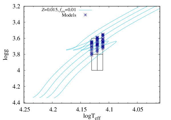
Table 8 is organised as follows:
- •
Column 1: evolutionary phase of the model.
- •
Column 2: exponential overshooting parameter, .
- •
Column 3: initial abundances of hydrogen, .
- •
Column 4: initial abundances of helium, .
- •
Column 5: metallicity, .
- •
Column 6: stellar mass, [M☉].
- •
Column 7: age, calculated from cloud collapse [Myr].
- •
Column 8: effective temperature.
- •
Column 9: luminosity.
- •
Column 10: radius.
- •
Column 11: surface gravity.
- •
Column 12: central hydrogen content, .
- •
Column 13: surface rotational velocity, [km s-1].
| Evol. Phase | age | |||||||||||
|---|---|---|---|---|---|---|---|---|---|---|---|---|
| [Myr] | km s-1] | |||||||||||
| MS | 0.01 | 0.7 | 0.285 | 0.015 | 4.2954 | 111.618 | 4.1304 | 2.7507 | 4.3421 | 3.7955 | 0.1913 | 54.35 |
| MS | 0.01 | 0.7 | 0.285 | 0.015 | 4.4756 | 105.722 | 4.1304 | 2.8338 | 4.7783 | 3.7302 | 0.1415 | 59.81 |
| MS | 0.01 | 0.7 | 0.285 | 0.015 | 4.6643 | 99.587 | 4.1304 | 2.9169 | 5.2580 | 3.6650 | 0.0900 | 65.81 |
| MS | 0.01 | 0.7 | 0.285 | 0.015 | 4.2686 | 116.985 | 4.1206 | 2.7507 | 4.5437 | 3.7533 | 0.1582 | 56.88 |
| MS | 0.01 | 0.7 | 0.285 | 0.015 | 4.4489 | 110.208 | 4.1206 | 2.8338 | 5.0003 | 3.6882 | 0.1080 | 62.59 |
| MS | 0.01 | 0.7 | 0.285 | 0.015 | 4.2444 | 122.048 | 4.1107 | 2.7507 | 4.7559 | 3.7113 | 0.1250 | 59.53 |
| CoP | 0.01 | 0.7 | 0.285 | 0.015 | 4.2398 | 132.385 | 4.1304 | 2.8338 | 4.7781 | 3.7067 | 0.0020 | 59.81 |
| CoP | 0.01 | 0.7 | 0.285 | 0.015 | 4.5359 | 111.943 | 4.1304 | 2.9169 | 5.2581 | 3.6529 | 0.0081 | 65.81 |
| CoP | 0.01 | 0.7 | 0.285 | 0.015 | 4.2909 | 128.383 | 4.1206 | 2.8338 | 5.0003 | 3.6724 | 0.0052 | 62.59 |
| CoP | 0.01 | 0.7 | 0.285 | 0.015 | 4.5940 | 107.533 | 4.1206 | 2.9169 | 5.5024 | 3.6190 | 0.0267 | 68.88 |
| CoP | 0.01 | 0.7 | 0.285 | 0.015 | 4.4194 | 115.009 | 4.1107 | 2.8338 | 5.2328 | 3.6458 | 0.0711 | 65.50 |
| CoP | 0.01 | 0.7 | 0.285 | 0.015 | 4.3365 | 124.658 | 4.1107 | 2.8338 | 5.2328 | 3.6376 | 0.0129 | 65.50 |
| AtL | 0.01 | 0.7 | 0.285 | 0.015 | 4.2527 | 131.567 | 4.1304 | 2.8338 | 4.7772 | 3.7081 | 0.0000 | 59.85 |
| AtL | 0.01 | 0.7 | 0.285 | 0.015 | 4.4173 | 119.957 | 4.1304 | 2.9169 | 5.2581 | 3.6414 | 0.0000 | 65.81 |
| AtL | 0.01 | 0.7 | 0.285 | 0.015 | 4.2186 | 134.288 | 4.1206 | 2.8338 | 5.0017 | 3.6650 | 0.0000 | 62.58 |
| AtL | 0.01 | 0.7 | 0.285 | 0.015 | 4.3784 | 122.679 | 4.1206 | 2.9169 | 5.5026 | 3.5981 | 0.0000 | 68.90 |
| AtL | 0.01 | 0.7 | 0.285 | 0.015 | 4.3525 | 124.607 | 4.1107 | 2.9169 | 5.7585 | 3.5560 | 0.0000 | 72.11 |
| MS | 0.01 | 0.73 | 0.255 | 0.015 | 4.4641 | 115.587 | 4.1304 | 2.7507 | 4.3421 | 3.8122 | 0.2239 | 54.35 |
| MS | 0.01 | 0.73 | 0.255 | 0.015 | 4.6520 | 109.649 | 4.1304 | 2.8338 | 4.7780 | 3.7470 | 0.1735 | 59.80 |
| MS | 0.01 | 0.73 | 0.255 | 0.015 | 4.8523 | 103.060 | 4.1304 | 2.9169 | 5.2581 | 3.6822 | 0.1244 | 65.81 |
| MS | 0.01 | 0.73 | 0.255 | 0.015 | 4.4364 | 121.321 | 4.1206 | 2.7507 | 4.5440 | 3.7700 | 0.1901 | 56.88 |
| MS | 0.01 | 0.73 | 0.255 | 0.015 | 4.6263 | 114.228 | 4.1206 | 2.8338 | 5.0004 | 3.7051 | 0.1408 | 62.59 |
| MS | 0.01 | 0.73 | 0.255 | 0.015 | 4.8240 | 107.087 | 4.1206 | 2.9169 | 5.5027 | 3.6402 | 0.0901 | 68.86 |
| MS | 0.01 | 0.73 | 0.255 | 0.015 | 4.4118 | 126.589 | 4.1107 | 2.7507 | 4.7554 | 3.7281 | 0.1573 | 59.52 |
| MS | 0.01 | 0.73 | 0.255 | 0.015 | 4.6017 | 118.613 | 4.1107 | 2.8338 | 5.2328 | 3.6633 | 0.1078 | 65.50 |
| CoP | 0.01 | 0.73 | 0.255 | 0.015 | 4.1389 | 163.798 | 4.1107 | 2.7507 | 4.7553 | 3.7004 | 0.0010 | 59.52 |
| CoP | 0.01 | 0.73 | 0.255 | 0.015 | 4.4414 | 137.327 | 4.1107 | 2.8338 | 5.2334 | 3.6479 | 0.0050 | 65.51 |
| CoP | 0.01 | 0.73 | 0.255 | 0.015 | 4.3877 | 141.635 | 4.1206 | 2.8338 | 5.0005 | 3.6821 | 0.0019 | 62.59 |
| CoP | 0.01 | 0.73 | 0.255 | 0.015 | 4.6936 | 119.839 | 4.1206 | 2.9169 | 5.5026 | 3.6283 | 0.0077 | 68.87 |
| CoP | 0.01 | 0.73 | 0.255 | 0.015 | 4.6439 | 123.183 | 4.1304 | 2.9169 | 5.2576 | 3.6632 | 0.0032 | 65.81 |
| AtL | 0.01 | 0.73 | 0.255 | 0.015 | 4.1860 | 159.339 | 4.1107 | 2.7507 | 4.7555 | 3.7053 | 0.0000 | 59.52 |
| AtL | 0.01 | 0.73 | 0.255 | 0.015 | 4.3838 | 142.203 | 4.1107 | 2.8338 | 5.2319 | 3.6423 | 0.0000 | 65.49 |
| AtL | 0.01 | 0.73 | 0.255 | 0.015 | 4.5524 | 129.752 | 4.1107 | 2.9169 | 5.7573 | 3.5756 | 0.0000 | 72.08 |
| AtL | 0.01 | 0.73 | 0.255 | 0.015 | 4.4140 | 139.740 | 4.1206 | 2.8338 | 4.9996 | 3.6847 | 0.0000 | 62.60 |
| AtL | 0.01 | 0.73 | 0.255 | 0.015 | 4.5926 | 126.891 | 4.1206 | 2.9169 | 5.5026 | 3.6188 | 0.0000 | 68.86 |
| AtL | 0.01 | 0.73 | 0.255 | 0.015 | 4.6343 | 124.044 | 4.1304 | 2.9168 | 5.2565 | 3.6623 | 0.0000 | 65.78 |
| MS | 0.02 | 0.7 | 0.285 | 0.015 | 4.2140 | 124.052 | 4.1304 | 2.7507 | 4.3422 | 3.7872 | 0.2346 | 54.34 |
| MS | 0.02 | 0.7 | 0.285 | 0.015 | 4.5657 | 110.601 | 4.1304 | 2.9169 | 5.2580 | 3.6558 | 0.1512 | 65.81 |
| MS | 0.02 | 0.7 | 0.285 | 0.015 | 4.1830 | 130.318 | 4.1206 | 2.7507 | 4.5440 | 3.7445 | 0.2059 | 56.89 |
| MS | 0.02 | 0.7 | 0.285 | 0.015 | 4.3548 | 122.721 | 4.1206 | 2.8338 | 5.0003 | 3.6789 | 0.1649 | 62.59 |
| MS | 0.02 | 0.7 | 0.285 | 0.015 | 4.5385 | 114.612 | 4.1206 | 2.9169 | 5.5025 | 3.6137 | 0.1253 | 68.87 |
| MS | 0.02 | 0.7 | 0.285 | 0.015 | 4.1556 | 136.023 | 4.1107 | 2.7507 | 4.7554 | 3.7022 | 0.1786 | 59.59 |
| MS | 0.02 | 0.7 | 0.285 | 0.015 | 4.3290 | 127.323 | 4.1107 | 2.8338 | 5.2328 | 3.6368 | 0.1389 | 65.50 |
| MS | 0.02 | 0.7 | 0.285 | 0.015 | 4.5123 | 118.504 | 4.1107 | 2.9169 | 5.7580 | 3.5717 | 0.0993 | 72.07 |
| CoP | 0.02 | 0.7 | 0.285 | 0.015 | 4.0160 | 167.176 | 4.1107 | 2.8338 | 5.2328 | 3.6042 | 0.0005 | 65.50 |
| CoP | 0.02 | 0.7 | 0.285 | 0.015 | 4.3167 | 139.687 | 4.1107 | 2.9169 | 5.7585 | 3.5524 | 0.0030 | 72.07 |
| CoP | 0.02 | 0.7 | 0.285 | 0.015 | 4.2615 | 144.241 | 4.1206 | 2.9169 | 5.5025 | 3.5863 | 0.0011 | 68.88 |
| AtL | 0.02 | 0.7 | 0.285 | 0.015 | 4.0855 | 160.219 | 4.1107 | 2.8338 | 5.2328 | 3.6117 | 0.0000 | 65.51 |
| AtL | 0.02 | 0.7 | 0.285 | 0.015 | 4.3141 | 140.130 | 4.1107 | 2.9169 | 5.7580 | 3.5522 | 0.0000 | 72.05 |
| AtL | 0.02 | 0.7 | 0.285 | 0.015 | 4.3173 | 139.798 | 4.1206 | 2.9169 | 5.5019 | 3.5920 | 0.0000 | 68.88 |
| MS | 0.01 | 0.7 | 0.29 | 0.01 | 4.0943 | 119.097 | 4.1304 | 2.7507 | 4.3422 | 3.7747 | 0.1281 | 54.35 |
| MS | 0.01 | 0.7 | 0.29 | 0.01 | 4.0678 | 124.309 | 4.1206 | 2.7507 | 4.5440 | 3.7324 | 0.0922 | 56.87 |
| CoP | 0.01 | 0.7 | 0.29 | 0.01 | 3.9166 | 143.624 | 4.1304 | 2.7507 | 4.3424 | 3.7554 | 0.0035 | 54.35 |
| CoP | 0.01 | 0.7 | 0.29 | 0.01 | 3.9573 | 139.820 | 4.1206 | 2.7507 | 4.5446 | 3.7204 | 0.0084 | 56.88 |
| CoP | 0.01 | 0.7 | 0.29 | 0.01 | 4.0084 | 134.090 | 4.1107 | 2.7507 | 4.7553 | 3.6865 | 0.0287 | 59.52 |
| AtL | 0.01 | 0.7 | 0.29 | 0.01 | 3.8816 | 147.051 | 4.1304 | 2.7507 | 4.3408 | 3.7515 | 0.0000 | 54.38 |
| AtL | 0.01 | 0.7 | 0.29 | 0.01 | 4.0252 | 134.829 | 4.1304 | 2.8338 | 4.7782 | 3.6842 | 0.0000 | 59.81 |
| AtL | 0.01 | 0.7 | 0.29 | 0.01 | 4.1974 | 122.101 | 4.1304 | 2.9169 | 5.2582 | 3.6192 | 0.0000 | 65.81 |
| AtL | 0.01 | 0.7 | 0.29 | 0.01 | 3.8386 | 151.227 | 4.1206 | 2.7507 | 4.5442 | 3.7072 | 0.0000 | 56.87 |
| AtL | 0.01 | 0.7 | 0.29 | 0.01 | 3.9951 | 137.445 | 4.1206 | 2.8338 | 5.0008 | 3.6414 | 0.0000 | 62.59 |
| AtL | 0.01 | 0.7 | 0.29 | 0.01 | 4.1789 | 123.516 | 4.1206 | 2.9169 | 5.5025 | 3.5778 | 0.0000 | 68.87 |
| AtL | 0.01 | 0.7 | 0.29 | 0.01 | 3.8060 | 154.538 | 4.1107 | 2.7507 | 4.7560 | 3.6640 | 0.0000 | 59.50 |
| AtL | 0.01 | 0.7 | 0.29 | 0.01 | 3.9756 | 139.223 | 4.1107 | 2.8338 | 5.2336 | 3.5998 | 0.0000 | 65.49 |