Heterogeneous Idealization of Ion Channel Recordings - Open Channel Noise

To detect events on larger temporal scales, we use a modification of the Heterogeneous Simulataneous MUltiscale Change-point Estimator, $\operatorname{HSMUCE}$ from (Pein et al., 2017), which is a multiresolution procedure that is robust against heterogeneous noise. To avoid false positives due to the filter, we omit on each interval the first $m$ observations and do not test on very short intervals. Since we truncated the filter, the signal and the convolution of the signal with the lowpass filter differ only at the beginning of each segment. More precisely, if the signal is constant on an interval $[i/f_{\boldsymbol{s}},j/f_{\boldsymbol{s}}]$ with conductance level $c_{ij}$ and the first $m$ observations $Y_{i},\ldots,Y_{i+m-1}$ are ignored, all other observations $Y_{i+m},\ldots,Y_{j}$ have constant expectation equal to the conductance level $c_{ij}$. Hence, we take into account only intervals longer than $m/f_{\boldsymbol{s}}$ and ignore the first $m$ observations of each interval.
This leads to an estimator that detects change-points at presence of heterogeneous noise and filtering, i.e., when the heterogeneous ion channel model from Section II is assumed, while at the same time the probability to overestimate the number of events is controlled, i.e., a false positive is only added with probability at most equal to the tuning parameter $\alpha_{1}$, see Theorem VII.1 in Section VII in the supplement. A detailed definition of this estimator is given in Section VII in the supplement. Note that it does not take into account the convolution explicitly but still has good detection properties if events are long enough, but almost no detection power on small scales. Simulations (not displayed) show that for our data set events with of length at least $6.5\text{\,}\mathrm{ms}$, corresponding to $65$ sampling points, are detected reliably.
In the following two sections we will present a refinement of this idealization to detect and idealize events on smaller time scales, too, which proves to be relevant for our data example. Note that in this section and in the next section (a refinement will be provided in the local deconvolution step) we restrict all changes to the grid on which the observations are given, in other words, we assume that $f_{\boldsymbol{s}}\tau_{i}$ are integers.

To detect short events, we test on all intervals containing $l=1,\ldots,l_{\max}$ (to be defined later) observations whether the previous idealization is the underlying signal or whether the inclusion of an additional event on the considered interval is significantly better. More precisely, let $[\tau_{L},\tau_{R}]=[i/f_{\boldsymbol{s}},j/f_{\boldsymbol{s}}]$ be the interval on which we test. And assume for the moment that $\tau$ is the only change in $[(i-m+1)/f_{\boldsymbol{s}},(j+m-1)/f_{\boldsymbol{s}}]$ with conductance levels $c_{L}$ before and $c_{R}$ afterwards. Note that this also includes the scenario of no change in $[(i-m+1)/f_{\boldsymbol{s}},(j+m-1)/f_{\boldsymbol{s}}]$ by setting $c_{L}=c_{R}$. Then, we decide whether an additional event on $[\tau_{L},\tau_{R}]$ is required by testing the hypothesis

against the alternative

with $c\in\mathbb{R}$ arbitrary. The same structure is assumed for standard deviation functions $\sigma_{0}$ and $\sigma_{1}$ with values $s_{L},s$ and $s_{R}$. The precise hypotheses and alternatives, i.e., the values for $\tau,c_{L},c_{R},s_{L}$ and $s_{R}$, are determined by the previous idealization step. If more than one change is contained in $[(i-m+1)/f_{\boldsymbol{s}},(j+m-1)/f_{\boldsymbol{s}}]$, no local test will be performed on this interval. The reasoning behind this and how to obtain $\tau,c_{L},c_{R},s_{L}$ and $s_{R}$ exactly are explained in the paragraph ’Obtaining the hypotheses and alternatives’ in Section VIII in the supplement. All tests are performed at simultaneous error level $\alpha_{2}>0$.
The form of these hypotheses allows us to construct a test statistic that takes into account the convolution explicitly. Moreover, information provided by potential variance changes can be used as well. We provide details of the corresponding test in the paragraph ’Local testing’ in Section VIII in the supplement. All choices there are motivated by a trade-off between a good detection power for events in the measurements in Section V, see Figure 1, and a reasonable computational complexity.
If a hypothesis is rejected, we replace the single change-point at $\tau$ by a short peak. Temporary locations will be placed at $\tau_{L}=i/f_{\boldsymbol{s}}$ and $\tau_{R}=j/sr$, but exact locations and the conductance level $c$ will be obtained in the upcoming deconvolution step. However, note that usually one event in the data causes rejections of multiple tests. Therefore, we only consider the event with the largest test statistic among all rejections on intervals that intersect or adjoin each other. More details are provided in the paragraph ’Multiple dependent rejections’ in Section VIII in the supplement.

The final idealization is obtained by local deconvolution as described in Section 3.2 of (Pein et al., 2018) with two adjustments, which will be discussed in Section IX in the supplement. This means in particular that we still use the likelihood function of observations with homogeneous noise, although heterogeneous noise is assumed. Simulations show, see Section IV, that this works reasonably well for the recordings we analyze in Section V. Alternatives for recordings with more pronounced noise heterogeneity are discussed in Section VI-A.

The multiresolution regression step in Section III-A can be computed by a pruned dynamic program as described in Section A.1 in the supplement of (Pein et al., 2017). For related ideas, see also (Killick et al., 2012; Frick et al., 2014; Li et al., 2016; Maidstone et al., 2017) and the references given there. The implementation of the local tests in Section III-B is straightforward. The local deconvolution in Section III-C can be computed by an iterative grid search as described in Section 3.2 of (Pein et al., 2018). An implementation of $\operatorname{HILDE}$ is available by the R function hilde in the package clampSeg. The package is available on request and has been submitted parallel to CRAN (Pein et al., 2019b). All run time critical parts are written in C++ and are interfaced by the R code.
The worse case computation complexity of the dynamic program is quadratic in the number of observations $n$. However, in most ion channel recordings conductance changes occur frequently which reduces the complexity to be linear $\mathcal{O}(n)$, see Section A.3 in the supplement of Pein et al., 2017. The local tests in Section III-B are of complexity $\mathcal{O}(l_{\max}^{2}n)$, since for each of the $l_{\max}$ scales $1,\ldots,l_{\max}$ roughly $n$ tests have to be performed and the complexity to compute a single test is at most of order $\mathcal{O}(l_{\max})$. The computation time of the local deconvolution is dominated by the iterative grid search to deconvolve a single event. The deconvolution of a single event is constant in the number of observations, since the number of involved observations and the grid sizes do not increase. Moreover, the number of involved observations is small and the covariance matrix is a band matrix, with band size equal to $m$, which allows fast computation. Hence, the complexity of the deconvolution increases linearly in the number of events which increases for ion channel recordings typically linearly in the number of observations. In summary, for a typical channel trace the complexity to compute $\operatorname{HILDE}$ increases only linearly in the number of observations. This is confirmed by a run time of less than five minutes for idealizing the $600\,000$ observations in Figure 1 on a Dell Latitude E6530 with Intel(R) Core(TM) i5-3340M CPU 2.70GHz processor. Similar run times are obtained for the traces generated in Section IV-D. Thus, the theoretical considerations as well as the empirical run times confirm that $\operatorname{HILDE}$ can be computed efficiently, which is important since large data sets have to be analyzed.

$\operatorname{HILDE}$ can be tuned by the parameters $\alpha_{1},\alpha_{2},l_{\max}$ and $\gamma^{2}$, see Algorithm 1 and the referenced sections for a definition. The probability to overestimate the number of conductance changes is approximately controlled by the sum of the error levels $\alpha=\alpha_{1}+\alpha_{2}$. Hence, if such an overestimation control is desired, $\alpha$ should be chosen small. As a default choice we suggest $\alpha=0.05$. Increasing $\alpha$ yields to a larger detection power (at the price of including more false positives). Hence, one may ’screen’ for different $\alpha$ if important events are difficult to detect. The levels $\alpha_{1}$ and $\alpha_{2}$ allocates the power between the multiresolution test for detecting events on large scales ($>l_{\max}$) and the local tests to detect events on small scales ($\leq l_{\max}$). We have chosen $\alpha_{2}=0.04$ and $\alpha_{1}=0.01$ in our data analysis, since our focus was on detecting short events primarily, while events on larger scales were easier to detect. More weight can be put on $\alpha_{1}$ if either short events are of less interest or if long events are difficult to detect as well, e.g. since they have a smaller jump size than the short events. The latter is often called subgating and was for instance studied in (Hotz et al., 2013). The tuning parameter $l_{\max}$, the largest scale on which local tests are performed to find short events, should be chosen such that all events on larger scales are detected by the previous multiresolution test. This can for instance be determined by Monte-Carlo simulations. In our setting, we choose $l_{\max}=65$, since simulations (not displayed) showed that the multiresolution step in Section III-A is able to detect events which contain more than $65$ observations with probability almost one. The correlation matrix is regularized with parameter $\gamma^{2}=1$, further details can be found in Section III B in (Pein et al., 2018). And, as mentioned before, we truncate the kernel and autocorrelation function of the filter at $m=11$ as the autocorrelation function is below $10^{-3}$ afterwards. All of these choices are the default parameters of the function hilde and are used in the simulations in Section IV and in the real data application in Section V.

We generate all signals and observations accordingly to the heterogeneous ion channel model we described in Section II and such that they are in line with the measured data we analyze in Section V. This means in particular that amplitudes, dwell times and noise levels of the generated observations are chosen such that they are similar to those of the analyzed datasets. We also simulate a 4-pole Bessel filter with $1\text{\,}\mathrm{kHz}$ cut-off frequency and sample the observation at $10\text{\,}\mathrm{kHz}$.
The expectation of the observations, given by the convolution of the signal with the truncated kernel $F_{m}$ of the lowpass Bessel filter, can be computed explicitly. For the errors we oversample by a factor of $100$, i.e., we generate $100$ times as many independent Gaussian observations, discretize the filter accordingly, compute a discrete convolution and rescale the observations such that they have the desired standard deviation.

In this simulation with $4\,000$ observations we examine the detection and idealization of a single isolated peak. More precisely, in accordance with the model in Section II and with the estimated values in Section V for the observations in Figure 1, we choose conductance levels $c_{0}=c_{2}=0$, $c_{1}=0.32$, variances $s_{0}^{2}=s_{2}^{2}=6.1\cdot 10^{-5}$ and varying variance $s_{1}^{2}\in\{2\cdot 10^{-4},5\cdot 10^{-4},10^{-3},2\cdot 10^{-3},5\cdot 10^{-3}\}$ to examine the influence of different noise levels. Note that $s_{1}^{2}=10^{-3}$ is roughly the noise level in the measurements in Section V. Moreover, we simulate changes at $\tau_{1}=2000/f_{\boldsymbol{s}}$ and $\tau_{2}=(2000+\ell)/f_{\boldsymbol{s}}$, c.f. (II.1), and are interested in how well $\operatorname{HILDE}$ detects the peak and idealizes the locations $\tau_{1}$ and $\tau_{2}$ and the level $l_{1}$ as a function of $\ell$, the length (relative to the sampling rate $f_{\boldsymbol{s}}$) of the peak. For $\ell=5$, Figure 6 shows an example of the simulated data as well as the idealizations by $\operatorname{HILDE}$ and their convolutions with the Bessel filter in a neighborhood of the peak. Tables I-III summarize our results based on $10\,000$ repetitions for $\ell=2,3,5$.
To this end, we count how often the signal is correctly identified, i.e., only the peak and no other change is detected. More precisely, we define the peak as detected if there exists a $j$ such that $|\hat{\tau}_{j}-\tau_{1}|<m/f_{\boldsymbol{s}}$ and $|\hat{\tau}_{j+1}-\tau_{2}|<m/f_{\boldsymbol{s}}$ as a peak is shifted at most $m/f_{\boldsymbol{s}}$ by the filter. If only one change but not a peak is within these boundaries we do not count it as a true detection, but also not as a false positive, whereas all other changes are counted as false positives. For the estimated locations and the level we only consider cases where the peak is detected and report the mean square error, the bias and the standard deviation.

In most scenarios, $\operatorname{HILDE}$ has a good detection power and detects almost no false positives, see Table I. Only for a five times larger variance than in the real data and when $l\leq 3$ few events are missed. In Tables II and III we found that idealization of the locations $\tau_{1}$ and $\tau_{2}$ and the conductance value $c_{1}$ works well for variances similar to the real data, but has some issues when the variance of the peak is larger, in particular in the scenario of a five times larger variance. For such observations it might be desirable to take into account the heterogeneous noise in the deconvolution step, see Section VI-A for more details. For smaller variances the results for estimating the locations are better when the peak is longer, but for larger variances results are even worse when the peak is longer. An explanation might be two effects with opposite influences. The conductance change provide more information when the peak is longer, but then also the overall variance of the observations is larger which reduces estimation accuracy. Estimation of the level $c_{1}$ is always more accurate when the peak is longer. It seems that here the first effect dominates.
All in all, these simulations confirm that $\operatorname{HILDE}$ performs very well for observations comparable to them in Section V.

To examine how well $\operatorname{HILDE}$ separates two consecutive peaks we perform the same simulations as in Section 4.3 in (Pein et al., 2018), since results are identical for homogeneous and heterogeneous noise as separation depends on the method and distance between the peaks but not on the noise level. More precisely, we consider a signal $f$ with changes at $\tau_{1}=2\,000/f_{\boldsymbol{s}}$, $\tau_{2}=\tau_{1}+5/f_{\boldsymbol{s}}$, $\tau_{3}=\tau_{2}+d$ and $\tau_{4}=\tau_{3}+5/f_{\boldsymbol{s}}$, , with $\tau_{0}=0$ and $\tau_{\operatorname{end}}=4\,000/f_{\boldsymbol{s}}$ and levels $l_{0}=l_{2}=l_{4}=$40\text{\,}\mathrm{pS}$$ and $l_{1}=l_{3}=$20\text{\,}\mathrm{pS}$$. Hence $d$ is the distance between the two peaks. We distinguish between perfect separation, i.e., the detection step of $\operatorname{HILDE}$ identifies the two peaks (4 changes) and the local deconvolution yields idealizations for the four levels (illustrated in Figure 7(c)). Secondly, separation fails in the detection step, i.e., the multiresolution reconstruction recognizes only 2 changes and identifies one peak whose level can be further deconvolved (illustrated in Figure 7(a)). Finally, separation fails in the deconvolution step, i.e., $\operatorname{HILDE}$ identifies two peaks but the distance is so small that the deconvolution step cannot separate them, in other words, no long segment is in between (illustrated in Figure 7(b)).

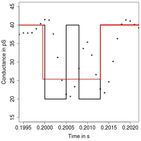
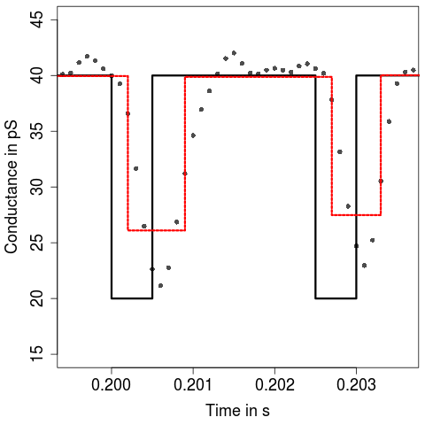
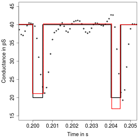
Figure 8 shows the frequency at which each scenario occurred as a function of $d$, the distance between the two peaks, in $10\,000$ simulations for each value of $d=\{1,2,\ldots,70\}$. We found that the two peaks are detected if $d>6$, but separation in the detection step and hence an appropriate idealization requires $d\geq 62$. Hence, in Section V events have to be separated by more than $6.2\text{\,}\mathrm{ms}$ to be idealized appropriately. In comparison, we found that events are on average separated by $$1/(2.67+4.50)\text{\,}\mathrm{s}$\approx$0.14\text{\,}\mathrm{s}$$ which shows that this limitation is not an issue for the analyzed PorB recordings.

In this section we simulate data from a three state hidden Markov model. Since hidden Markov models are often assumed for ion channel recordings, it is instructive to investigate the methods in such a scenario. We simulate observations that resemble the PorB data we analyze in Section V. More precisely, we have expectations $0\text{\,}\mathrm{nS}$, $0\text{\,}\mathrm{nS}$ and $0.32\text{\,}\mathrm{nS}$ as well as standard deviations $0.0078\text{\,}\mathrm{nS}$, $0.0078\text{\,}\mathrm{nS}$ and $0.0316\text{\,}\mathrm{nS}$, i.e. the variances are $6.1\cdot 10^{-5}\text{\,}\mathrm{(}\mathrm{n}\mathrm{S}\mathrm{)}^{2}$ and $10^{-3}\text{\,}\mathrm{(}\mathrm{n}\mathrm{S}\mathrm{)}^{2}$. The dwell times in the first, second and third state are exponentially distributed with rates $20\text{\,}\mathrm{Hz}$, $400\text{\,}\mathrm{Hz}$ and $7\text{\,}\mathrm{Hz}$, respectively. The process always jumps from the first or second state to the third state, i.e., no transitions between the first and second state are allowed. And it jumps from the third state with probability $2/3$ to the first state and with probability $1/3$ to the second state. We generate five time series with $600\,000$ observations, each. Each trace looks similar to the observations in Figure 1 and hence we refrain from showing an example.
We analyze these data sets with $\operatorname{HILDE}$ and for purpose of comparison with $\operatorname{JULES}$ (Pein et al., 2018), $\operatorname{HSMUCE}$ (Pein et al., 2017) and an HMM based approach which assumes the true three state model, i.e. three states, whereby two have the same expectations and variances and no transitions are allowed between them. We used

as starting values for the Baum-Welch algorithm. Those standard deviations were determined by taking the empirical standard deviation of all observations below and above $0.2$, respectively. Idealizations are obtained by using a Viterbi algorithm.
The Baum-Welch algorithm estimated the following parameters

We will discuss the estimated transition matrix later in comparison with the other approaches and when we also discuss the results using the Viterbi algorithm. The estimated expectations and standard deviations are accurate. For the other approaches we show in Figure 9 histograms of the estimated amplitudes of all events with an amplitude between $0.2\text{\,}\mathrm{nS}$ and $0.5\text{\,}\mathrm{nS}$.

We found in Figure 9 that all approaches estimate the amplitude accurately. The estimated amplitudes of $\operatorname{HSMUCE}$ are skewed, but the final estimation is still decent.
We continue with an analysis of the dwell times. To this end, we consider from now on all events with estimated conductance level between $-0.05\text{\,}\mathrm{nS}$ and $0.05\text{\,}\mathrm{nS}$ as a closed event and between $0.15\text{\,}\mathrm{nS}$ and $2\text{\,}\mathrm{nS}$ as an open event, while all other events are considered as artifacts and are ignored. Figure 10 shows histograms of the dwell times in the closed state for various approaches.

We see that with the exception of $\operatorname{HSMUCE}$ (it misses short events) none on the histograms look exponentially distributed, since we have a mixture of short and long events. Hence, in Figures 11 and 12 we will analyze short and long events separately. To this end, we say an event is short if its dwell time is between $0.1\text{\,}\mathrm{ms}$ and $5\text{\,}\mathrm{ms}$ and long if its dwell time is between $20\text{\,}\mathrm{ms}$ and $200\text{\,}\mathrm{ms}$. To estimate the rates, we apply a missed event correction like in (Pein et al., 2018).

We found from Figures 11 and 12 that $\operatorname{HILDE}$ recovers in both cases the exponential distribution very well and estimates both rates of $400\text{\,}\mathrm{Hz}$ and $20\text{\,}\mathrm{Hz}$ with $332.59\text{\,}\mathrm{Hz}$ and $19.2629\text{\,}\mathrm{Hz}$ accurately. In comparison, $\operatorname{JULES}$ is not able to deconvolve all events due to the detection of additional spurious events, compare Figure 3. The rate for the short events is with $520.16\text{\,}\mathrm{Hz}$ still accurately, but the rate for the long events is with $9.0682\text{\,}\mathrm{Hz}$ significantly underestimated. Notably the dwell times are still (almost) exponentially distributed. $\operatorname{HSMUCE}$ misses short events, in total it has detected only $18$ short events. Hence, a rate for the short events cannot be estimated. The rate for the long events is with $6.0182\text{\,}\mathrm{Hz}$ underestimated as well. The hidden Markov approach estimated with $347.44\text{\,}\mathrm{Hz}$ and $19.3949\text{\,}\mathrm{Hz}$ both rates accurately. However, since this approach misses very short events, for the rate for the short events we had to apply a stricter missed event correction that takes into account only events with a length of at least $0.75\text{\,}\mathrm{ms}$. Hence, at least in the used form the hidden Markov approach is less favorable to analyze short events (since its corrected estimate is based on less event and hence will have a larger variance). This is remarkably, since the idealization on very short temporal scales is considered to be a strength of hidden Markov approaches. Finally, the estimated exit probabilities by the Baum-Welch algorithmus of $0.002671$ and $0.000644$ corresponds to estimated rates of $26.71\text{\,}\mathrm{Hz}$ and $6.44\text{\,}\mathrm{Hz}$ which is much worse than the rates estimated using the idealizations obtained by the Viterbi algorithm.
We are now analyzing how often closing events occur. To this end, we analyze the dwell times in the open state or in other words the distance between two closing events. Moreover, we analyze the proportions of short and long events. Therefore, we divide the number of detected events by the estimated probability that such an event is detected assuming an exponential distribution for the dwell times.

We found from Figure 13 that $\operatorname{HILDE}$, $\operatorname{HSMUCE}$ and the hidden Markov approach recover the exponential distribution very well and estimate the rate of $7\text{\,}\mathrm{Hz}$ with $6.4007\text{\,}\mathrm{Hz}$, $6.4919\text{\,}\mathrm{Hz}$ and $6.2389\text{\,}\mathrm{Hz}$ accurately. Only $\operatorname{JULES}$ underestimates the rate because of previously explained reasons with $4.3362\text{\,}\mathrm{Hz}$ a bit. $\operatorname{HILDE}$, $\operatorname{JULES}$ and $\operatorname{HMM}$ estimated with $0.3608$, $0.2982$ and $0.4082$, respectively, the proportion of short events decently, recall that the truth is $1/3$. This number could not be determined using $\operatorname{HSMUCE}$, since it misses almost all short events. Once again, the Baum-Welch provides with $27.06\text{\,}\mathrm{Hz}$ and $0.0329$ much worse results.
All in all, we found that $\operatorname{HILDE}$ was indeed able to recover all parameters very well. All other model-free idealization methods had at least one massive problem. The hidden Markov approach might be usable, but requires a more restrictive missed event correction and is also more complicated to apply. One should also keep in mind that we used the true parametric model class as prior knowledge.

The model we proposed in Section II is a good assumption for ion channel recording at presence of open channel noise. However, in some patch clamp recordings additional high frequency $f^{2}$ (violet) and long tailed $1/f$ (pink) noise components have been observed, for a more detailed discussion see (Neher and Sakmann, 1976; Venkataramanan et al., 1998b; Levis and Rae, 1993) and the references therein. Thereto, in this section we examine how robust $\operatorname{HILDE}$ is against such noise components. To this end, we revisit the simulation setting from Section IV-B with $s_{1}=10^{-3}$ only.
For the violet noise we use as suggested by (Venkataramanan et al., 1998a) a moving average process with coefficients $0.8$ and $-0.6$. For the pink noise we use the algorithm available on https://github.com/Stenzel/newshadeofpink. We assume that the pink noise is globally present. More precisely, we reduce the previously present noise by a factor of $1/2$ and add pink noise which is scaled such that its standard deviation is equal to $1/2\sqrt{6.1\cdot 10^{-5}}$ (half of the standard deviation in the background in Section IV-B). For the high frequency violet noise we consider the setting that the new noise component is state-dependent as well. In other words, we generated errors from such a moving average process and convolved them with the kernel of the lowpass filter instead of assuming white noise errors.

We found in Table IV that $\operatorname{HILDE}$ is very robust against the additional $f^{2}$ but effected by $1/f$ noise. At presence of the latter noise, the standard deviation estimation on the long segments is wrong which causes the detection of false positives in roughly a quarter of the cases. Note, that false positives are caused by the underestimated standard deviation but also by the long range dependency itself. However, the false positives have a small amplitude and therefore do not influence the analysis severely or can be removed by postfiltering. Parameter estimation (not displayed) is slightly effected by $1/f$ noise (estimation of the change-point locations is slightly worse, but estimation of the size of the change is even improved), but not affected by presence of $f^{2}$ noise.

We analyze single channel recordings of PorB from Neisseria meningitidis (recall the last paragraph in the introduction). In the following we analyze six traces, each of them is one minute long and consists of $600\,000$ observations. An example is shown in Figure 1, which shows distinct heterogeneous noise.
Measurements were performed on solvent-free planar bilayers using the Port-a-Patch (Nanion Technologies). Giant unilamellar vesicles (GUVs) composed of 1,2-diphytanoyl-sn-glycero-3-phosphocholine (DPhPC)/cholesterol (9:1) were prepared by electroformation (AC, U = 3 V, peak-to-peak, f = 5 Hz, t = 2 h) in the presence of 1 M sucrose at $20\text{\,}\mathrm{\SIUnitSymbolCelsius}$. Spreading of a GUV in $1\text{\,}\mathrm{\textsc{m}}$ KCl, $10\text{\,}\mathrm{m\textsc{m}}$ HEPES, pH 7.5 on an aperture (d = 1-5 $\mu$m) in a borosilicate chip by applying 10-40 mbar negative pressure resulted in a solvent-free membrane with a resistance in the G$\Omega$ range. Once the membrane with a G$\Omega$ seal was formed, varying amounts of a PorB stock solution (2.2 $\mu$M in 200 mM NaCl, 20 mM Tris, 0.1% (w/w) LDAO, pH 7.5) were added to the buffer solution (50 $\mu$L) at an applied DC potential of +40 mV. Current traces were recorded at a sampling rate of $10\text{\,}\mathrm{kHz}$ and filtered with a low-pass four-pole Bessel filter of $1\text{\,}\mathrm{kHz}$ using an Axopatch 200B amplifier (Axon Instruments). For digitalization, an A/D converter (Digidata 1322; Axon Instruments) was used.

Idealizations are obtained by $\operatorname{HILDE}$ with parameter choices as in Section III-E. Moreover, an illustrative comparison with other approaches was discussed in the introduction (recall Figures 19-4). In Figure 1 we see that the channel switches frequently between two conductance levels, roughly between $0.04\text{\,}\mathrm{nS}$ and $0.36\text{\,}\mathrm{nS}$, the variance is roughly $6.1\cdot 10^{-5}\text{\,}\mathrm{(}\mathrm{n}\mathrm{S}\mathrm{)}^{2}$ in the closed state and $10^{-3}\text{\,}\mathrm{(}\mathrm{n}\mathrm{S}\mathrm{)}^{2}$ in the open state. Moreover, several artifacts seem to be present, see for instance the fluctuating conductance in the open state in the first ten seconds. We stress that such artifacts heavily disturb any idealization that assumes a HMM, confer Figure 19. Contrarily, the model-free idealization by $\operatorname{HILDE}$ (Figure 5) recovers all visible features on small as well as on large temporal scales accurately. In particular, the zooms into single peaks (Figure 5, lower panels) shows that $\operatorname{HILDE}$ fits the observations well which is also a confirmation of our model. Since PorB forms three pores, four different conductance levels are possible. However, in this measurement we see only two different conductance levels. Such a cooperative opening and closing was observed before, see for instance (Song et al., 1998).

We now use the obtained idealizations to analyze the gating dynamics in a similar fashion as the simulated data in Section IV-D. We will focus in this section on $\operatorname{HILDE}$, but we will compare it in Section XI in the supplement with analyses based on $\operatorname{JULES}$, $\operatorname{HSMUCE}$ and $\operatorname{HMM}$. We say a channel opens (a gating event from the lower conductance level to the higher conductance level) if the idealized level is between $0.25\text{\,}\mathrm{nS}$ and $2\text{\,}\mathrm{nS}$ and the previous level is between $0\text{\,}\mathrm{nS}$ and $0.1\text{\,}\mathrm{nS}$. To study the amplitude, we consider the conductance difference of all such events. Figure 14 shows a histogram of the so obtained amplitudes between $0.2\text{\,}\mathrm{nS}$ and $0.5\text{\,}\mathrm{nS}$. All other events are either closing events or are considered as artifacts. Such artifacts can for instance be base line fluctuations as discussed in the introduction. We stress that an analysis of the closing events leads to very similar results.

The histogram in Figure 14 shows only one mode. Hence, all events have the same amplitude up to measurements and idealization errors. This means especially that also the flickering events are full-sized. An amplitude of $0.3194\text{\,}\mathrm{nS}$ is estimated by the half sample mode (Robertson and Cryer, 1974), computed in R by using the modeest package. Note that other mode estimators or Gaussian mean estimation lead to similar results. This amplitude coincides with the one obtained by a manual analysis using the pClamp 10.2 software package (Axon Instruments), see (Bartsch et al., 2019).
We now analyze the dwell time in the open state and how frequently the channel opens. We take into account events with an amplitude between $0.2\text{\,}\mathrm{nS}$ and $0.5\text{\,}\mathrm{nS}$ and with a dwell time between $0.1\text{\,}\mathrm{ms}$ and $200\text{\,}\mathrm{ms}$, since shorter events cannot be detected reliably and longer events are rare and often interrupted by artifacts. Histograms of the dwell time in the open state are shown in Figure 15 together with an exponential fit using a missed event correction like in (Pein et al., 2018).

Interestingly, the dwell times do not fit a single exponential distribution, but when we split the events in short (shorter than $5\text{\,}\mathrm{ms}$) and long (longer than $20\text{\,}\mathrm{ms}$) ones, both fit exponential distributions very well, with an estimated average duration of $51.62\text{\,}\mathrm{ms}$ and $2.31\text{\,}\mathrm{ms}$, respectively. Note, that these estimations are approximations, since an exponential distribution with a large / small rate generates with a small probability a long / short event, but since the average dwell times are very different this error is negligible. To best of our knowledge, fast and slow gating at the same time was not observed for PorB before. However, Grosse et al., 2014 showed that the loop within the pore structure of OmpG leads to fast flickering (fast time constant). If the loop is removed, there is still gating observed but less frequent (slower time constant). Even though this is not the same protein, in PorB we have a loop L3 which is also localized in the pore and forms an $\alpha$-helix in its center, which constricts the pore to its narrowest point. Hence, our findings support that similar dynamics might occur for PorB as well.
We are now analyzing the distance between two opening events. This is shown in Figure 16. Moreover, we analyze how many of the openings are short or long. Once again we apply a correction for missed events.

The distance between two events seem to be exponentially distributed and the estimated rate is $5.75\text{\,}\mathrm{Hz}$. We found that $39.08\%$ of all opening events were short events. Moreover, we found in Section XI in the supplement that all results obtained by $\operatorname{HILDE}$ could be confirmed by at least one other approach, but none of the other methods was able to reproduce all results obtained by $\operatorname{HILDE}$.

A different underlying interval set can be used for the multiresolution test. The set of all intervals of dyadic length provides in general a good compromise between detection power and computation time. But, if a larger detection power is required, the set of all intervals can be used at the price of a larger computational complexity. The other way around, if faster computation is demanded, a smaller interval set, for instance the dyadic partition like in (Pein et al., 2017), can be used. This might be particularly beneficial in situations in which the multiresolution test detects almost no events which results in a large computation time. Interesting alternatives are also the approaches in (Chan and Walther, 2013; Kovács et al., 2020) which require only a slightly larger computational effort than the use of all intervals of dyadic length but detects change-points in a certain sense statistically optimally. A different way to increase the detection power is to use likelihood ratio tests, again at computational expenses. We found in simulations (not displayed) that the likelihood ratio test statistic is slightly more powerful on small scales, but much slower to compute. However, a slightly worse detection power on small scales should not be a big concern, since a refinement by local tests will be done in the next step. Also for detecting events on small scales by local tests, see Section III-B, different statistics can be used to increase the detection power. For instance the likelihood ratio test or maximum likelihood estimators for the parameters $(c,s^{2})$ can be considered. However, they are computationally very demanding, since the likelihood function involves the inverse and the determinant of the covariance matrix given by (VIII.5).
Finally, our deconvolution approach assumes still homogeneous noise which we found in simulations works still well at presence of open channel noise, see Tables II and III. Taking into account the heterogeneous noise might be beneficial, in particular if the noise level differences are large, but difficult, maybe even impossible, since avoiding an ill-conditioned matrix by regularization and keeping the variance levels might be impossible to achieve at the same time.

We designed $\operatorname{HILDE}$ particularly to deal with heterogeneous noise. However, taking into account the convolution explicitly when detecting changes is also beneficial if the noise is homogeneous, i.e., a constant variance is assumed. In this situation, its detection power can be further improved by small modifications that utilize the assumption of a constant variance, they are explained in Section XII in the supplement. We found that $\operatorname{HILDE}$ has a better detection power than $\operatorname{JULES}$ (Pein et al., 2018), but at the price of worse separation properties and a larger computation time. More precisely, in the simulations in Section IV-B in (Pein et al., 2018) we found that $\operatorname{JULES}$ is able to detect an isolated peak of length $3.1/f_{\boldsymbol{s}}$ with probability almost one. In comparison, $\operatorname{HILDE}$ requires only $2.3/f_{\boldsymbol{s}}$ if homogeneous noise is assumed and $2.8/f_{\boldsymbol{s}}$ if heterogeneous noise is assumed (see Section 3.9.3. in (Pein, 2017)). Remarkably, the detection power of $\operatorname{HILDE}$ is even larger than the one of $\operatorname{JULES}$ if $\operatorname{HILDE}$ does not use the assumption of homogeneous noise which illustrates how much detection power is lost by not taking into account the convolution.

Our focus was on idealizing the conductance while the unknown variance was considered as a nuisance parameter. However, as a byproduct $\operatorname{HILDE}$ can easily be extended to an idealization of the variance which offers for instance a residual analysis of the noise to validate a given model. To this end, we use $\operatorname{HILDE}$ to estimate the change-point location of the conductance and assume that these are the change-points of the variance as well. Note that the model of Section II allows the variance to stay constant at such a location but precludes further variance changes. With the definitions from before (see Section III), if a segment is long, the square of the estimator in (VIII.1) can be used. Afterwards, the variance on short segments can be estimated by the estimator in (VIII.8). The resulting function will be an idealization of the variance.

References

- Ball and Rice, (1992) Ball, F. G. and Rice, J. A. (1992). Stochastic models for ion channels: introduction and bibliography. Math. Biosci., 112(2):189–206.
- Bartsch et al., (2019) Bartsch, A., Llabrés, S., Pein, F., Kattner, C., Schön, M., Diehn, M., Tanabe, M., Munk, A., Zachariae, U., and Steinem, C. (2019). High-resolution experimental and computational electrophysiology reveals weak -lactam binding events in the porin porB. Sci. Rep., 9(1):1264.
- Chan and Walther, (2013) Chan, H. P. and Walther, G. (2013). Detection with the scan and the average likelihood ratio. Stat. Sin., pages 409–428.
- Colquhoun, (1987) Colquhoun, D. (1987). Practical analysis of single channel records. Microelectrode techiques. The Plymouth workshop handbook. Cambridge: Company of Biologists.
- de Gunst et al., (2001) de Gunst, M. C. M., Künsch, H. R., and Schouten, J. G. (2001). Statistical analysis of ion channel data using hidden Markov models with correlated state-dependent noise and filtering. J. Am. Stat. Assoc., 96(455):805–815.
- Diehn, (2017) Diehn, M. (2017). Inference in Inhomogeneous Hidden Markov Models with Application to Ion Channel Data. PhD thesis, Georg-August-Universität Göttingen. http://hdl.handle.net/11858/00-1735-0000-0023-3FB4-2.
- Diehn et al., (2019) Diehn, M., Munk, A., and Rudolf, D. (2019). Maximum likelihood estimation in hidden markov Models with inhomogeneous noise. ESAIM: P&S, 23:492–523.
- Enikeeva et al., (2018) Enikeeva, F., Munk, A., and Werner, F. (2018). Bump detection in heterogeneous Gaussian regression. Bernoulli, 24(2):1266–1306.
- Frick et al., (2014) Frick, K., Munk, A., and Sieling, H. (2014). Multiscale change point inference (with discussion and rejoinder by the authors). J. R. Statist. Soc. B, 76(3):495–580.
- Fuliński et al., (1998) Fuliński, A., Grzywna, Z., Mellor, I., Siwy, Z., and Usherwood, P. N. R. (1998). Non-Markovian character of ionic current fluctuations in membrane channels. Phys. Rev. E, 58(1):919–924.
- Gnanasambandam et al., (2017) Gnanasambandam, R., Nielsen, M. S., Nicolai, C., Sachs, F., Hofgaard, J. P., and Dreyer, J. K. (2017). Unsupervised idealization of ion channel recordings by minimum description length: Application to human PIEZO1-channels. Front. Neuroinform., 11.
- Goychuk et al., (2005) Goychuk, I., Hänggi, P., Vega, J. L., and Miret-Artés, S. (2005). Non-Markovian stochastic resonance: Three-state model of ion channel gating. Phys. Rev. E, 71(6):061906.
- Grosse et al., (2014) Grosse, W., Psakis, G., Mertins, B., Reiss, P., Windisch, D., Brademann, F., Bürck, J., Ulrich, A., Koert, U., and Essen, L.-O. (2014). Structure-based engineering of a minimal porin reveals loop-independent channel closure. Biochemistry, 53(29):4826–4838.
- Hartel et al., (2019) Hartel, A. J. W., Shekar, S., Ong, P., Schroeder, I., Thiel, G., and Shepard, K. L. (2019). High bandwidth approaches in nanopore and ion channel recordings–A tutorial review. Anal. Chim. Acta.
- Heinemann and Sigworth, (1988) Heinemann, S. H. and Sigworth, F. J. (1988). Open channel noise. IV. Estimation of rapid kinetics of formamide block in gramicidin A channels. Biophys. J., 54(4):757–764.
- Heinemann and Sigworth, (1990) Heinemann, S. H. and Sigworth, F. J. (1990). Open channel noise. V. Fluctuating barriers to ion entry in gramicidin A channels. Biophys. J., 57(3):499–514.
- Heinemann and Sigworth, (1991) Heinemann, S. H. and Sigworth, F. J. (1991). Open channel noise. VI. Analysis of amplitude histograms to determine rapid kinetic parameters. Biophys. J., 60(3):577–587.
- Hotz et al., (2013) Hotz, T., Schütte, O. M., Sieling, H., Polupanow, T., Diederichsen, U., Steinem, C., and Munk, A. (2013). Idealizing ion channel recordings by a jump segmentation multiresolution filter. IEEE Trans. Nanobioscience, 12(4):376–386.
- Kass, (2005) Kass, R. S. (2005). The channelopathies: novel insights into molecular and genetic mechanisms of human disease. J. Clin. Invest., 115(8):1986–1989.
- Killick et al., (2012) Killick, R., Fearnhead, P., and Eckley, I. A. (2012). Optimal detection of changepoints with a linear computational cost. J. Am. Stat. Assoc., 107(500):1590–1598.
- Kovács et al., (2020) Kovács, S., Li, H., Bühlmann, P., and Munk, A. (2020). Seeded Binary Segmentation: A general methodology for fast and optimal change point detection. arXiv preprint arXiv:2002.06633.
- Levis and Rae, (1993) Levis, R. A. and Rae, J. L. (1993). The use of quartz patch pipettes for low noise single channel recording. Biophys. J., 65(4):1666–1677.
- Li et al., (2016) Li, H., Munk, A., and Sieling, H. (2016). FDR-control in multiscale change-point segmentation. Electron. J. Stat., 10(1):918–959.
- Maidstone et al., (2017) Maidstone, R., Hocking, T., Rigaill, G., and Fearnhead, P. (2017). On optimal multiple changepoint algorithms for large data. Stat. Comput., 27(2):519–533.
- Mercik and Weron, (2001) Mercik, S. and Weron, K. (2001). Stochastic origins of the long-range correlations of ionic current fluctuations in membrane channels. Phys. Rev. E, 63(5):051910.
- Neher and Sakmann, (1976) Neher, E. and Sakmann, B. (1976). Single-channel currents recorded from membrane of denervated frog muscle fibers. Nature, 260(5554):799–802.
- Overington et al., (2006) Overington, J. P., Al-Lazikani, B., and Hopkins, A. L. (2006). How many drug targets are there? Nat. Rev. Drug. Discov., 5(12):993–996.
- Pein, (2017) Pein, F. (2017). Heterogeneous Multiscale Change-Point Inference and its Application to Ion Channel Recordings. PhD thesis, Georg-August-Universität Göttingen. http://hdl.handle.net/11858/00-1735-0000-002E-E34A-7.
- (29) Pein, F., Hotz, T., Sieling, H., and Aspelmeier, T. (2019a). stepR: Multiscale change-point inference. R package version 2.1-0.
- (30) Pein, F., Hotz, T., Tecuapetla-Gómez, I., and Aspelmeier, T. (2019b). clampSeg: Idealisation of Patch Clamp Recordings. R package version 1.1-0.
- Pein et al., (2017) Pein, F., Sieling, H., and Munk, A. (2017). Heterogeneous change point inference. J. Roy. Statist. Soc. Ser. B, 79(4):1207–1227.
- Pein et al., (2018) Pein, F., Tecuapetla-Gómez, I., Schütte, O. M., Steinem, C., and Munk, A. (2018). Fully-automatic multiresolution idealization for filtered ion channel recordings: flickering event detection. IEEE Trans. Nanobioscience, 17(3):300–320.
- Qin et al., (2000) Qin, F., Auerbach, A., and Sachs, F. (2000). Hidden Markov modeling for single channel kinetics with filtering and correlated noise. Biophys. J., 79(4):1928–1944.
- Raj Singh et al., (2012) Raj Singh, P., Ceccarelli, M., Lovelle, M., Winterhalter, M., and Mahendran, K. R. (2012). Antibiotic permeation across the OmpF channel: modulation of the affinity site in the presence of magnesium. J. Phys. Chem. B, 116(15):4433–4438.
- Robertson and Cryer, (1974) Robertson, T. and Cryer, J. D. (1974). An iterative procedure for estimating the mode. J. Am. Stat. Assoc., 69(348):1012–1016.
- Sakmann and Neher, (1995) Sakmann, B. and Neher, E. (1995). Single-Channel Recording. Springer, 2nd. edition.
- Schroeder, (2015) Schroeder, I. (2015). How to resolve microsecond current fluctuations in single ion channels: The power of beta distributions. Channels, 9(5):262–280.
- Shelley et al., (2010) Shelley, C., Niu, X., Geng, Y., and Magleby, K. L. (2010). Coupling and cooperativity in voltage activation of a limited-state BK channel gating in saturating Ca2+. J. Gen. Physiol., 135(5):461–480.
- Siekmann et al., (2011) Siekmann, I., Wagner, L. E., Yule, D., Fox, C., Bryant, D., Crampin, E. J., and Sneyd, J. (2011). MCMC estimation of Markov models for ion channels. Biophys. J., 100(8):1919–1929.
- Sigworth, (1985) Sigworth, F. J. (1985). Open channel noise. I. Noise in acetylcholine receptor currents suggests conformational fluctuations. Biophys. J., 47(5):709–720.
- Sigworth, (1986) Sigworth, F. J. (1986). Open channel noise. II. A test for coupling between current fluctuations and conformational transitions in the acetylcholine receptor. Biophys. J., 49(5):1041–1046.
- Sigworth et al., (1987) Sigworth, F. J., Urry, D. W., and Prasad, K. U. (1987). Open channel noise. III. High-resolution recordings show rapid current fluctuations in gramicidin A and four chemical analogues. Biophys. J., 52(6):1055–1064.
- Song et al., (1998) Song, J., Minetti, C. A. S. A., Blake, M. S., and Colombini, M. (1998). Successful recovery of the normal electrophysiological properties of PorB (class 3) porin from Neisseria meningitidis after expression in Escherichia coli and renaturation. BBA Biomembranes, 1370(2):289–298.
- Tecuapetla-Gómez and Munk, (2017) Tecuapetla-Gómez, I. and Munk, A. (2017). Autocovariance estimation in regression with a discontinuous signal and m-dependent errors: A difference-based approach. Scand. J. Stat., 44(2):346–368.
- VanDongen, (1996) VanDongen, A. M. (1996). A new algorithm for idealizing single ion channel data containing multiple unknown conductance levels. Biophys. J., 70(3):1303–1315.
- (46) Venkataramanan, L., Kuc, R., and Sigworth, F. J. (1998a). Identification of hidden Markov models for ion channel currents. II. State-dependent excess noise. IEEE Trans. Signal Process., 46(7):1916–1929.
- Venkataramanan et al., (2000) Venkataramanan, L., Kuc, R., and Sigworth, F. J. (2000). Identification of hidden Markov models for ion channel currents. III. Bandlimited, sampled data. IEEE Trans. Signal Process., 48(2):376–385.
- (48) Venkataramanan, L., Walsh, J. L., Kuc, R., and Sigworth, F. J. (1998b). Identification of hidden Markov models for ion channel currents. I. Colored background noise. IEEE Trans. Signal Process., 46(7):1901–1915.
- Venkatraman et al., (2004) Venkatraman, E. S., Olshen, A. B., Lucito, R., and Wigler, M. (2004). Circular binary segmentation for the analysis of array-based DNA copy number data. Biostatistics, 5(4):557–572.
- Virji, (2009) Virji, M. (2009). Pathogenic neisseriae: surface modulation, pathogenesis and infection control. Nat. Rev. Microbiol., 7(4):274.
- Viterbi, (1967) Viterbi, A. (1967). Error bounds for convolutional codes and an asymptotically optimum decoding algorithm. IEEE Trans. Inf. Theory, 13(2):260–269.
- Yellen, (1984) Yellen, G. (1984). Ionic permeation and blockade in Ca2+-activated K+ channels of bovine chromaffin cells. J. Gen. Physiol., 84(2):157–186.
Supplement to