Optical Flow and Mode Selection for Learning-based Video CodingPubID: pubid: 978-1-7281-9320-5/20/$31.00 ©2020 IEEE
Abstract
This paper introduces a new method for inter-frame coding based on two complementary autoencoders: MOFNet and CodecNet. MOFNet aims at computing and conveying the Optical Flow and a pixel-wise coding Mode selection. The optical flow is used to perform a prediction of the frame to code. The coding mode selection enables competition between direct copy of the prediction or transmission through CodecNet.
The proposed coding scheme is assessed under the Challenge on Learned Image Compression 2020 (CLIC20) P-frame coding conditions, where it is shown to perform on par with the state-of-the-art video codec ITU/MPEG HEVC. Moreover, the possibility of copying the prediction enables to learn the optical flow in an end-to-end fashion i.e. without relying on pre-training and/or a dedicated loss term.
Index Terms:
Video Coding, Deep Learning, Mode Selection, Optical FlowI Introduction and Related Works
Video signals exhibit a high level of redundancies, leveraged by compression systems to reduce the transmission rate. Those redundancies can be classified into two categories, spatial or temporal. Classical video compression systems such as ITU/MPEG (AVC [1], HEVC [2] and VVC [3]) codecs reduce temporal redundancies through motion compensation. It relies on motion vectors, representing motion between reference frames (available at the decoder) and the current frame, which are estimated and conveyed as side-information. Motion vectors are used to perform a prediction of the current frame, allowing the system to transmit only the prediction error i.e. difference between the signal and its prediction (the residue), lowering the required rate. A frame coded without temporal dependency is called an intra frame in contrast to an inter frame relying on information from other frames.
Inspired by traditional codecs, most neural network-based video coding approaches [4, 5, 6, 7] also rely on motion compensation for inter frame processing. These methods use an optical flow network (such as SpyFlow [8] or PWC-Net [9]) to compute pixel-wise motion vectors. Motion vectors are transmitted by a dedicated neural-based coding system and used for motion compensation. The prediction is exploited through a simple encoding of the prediction error (difference between the frame and its prediction), computed either in image [4, 5] or in latent domain [6]. As stated in [10], it is not trivial to learn the optical flow with a loss function only based on the RD-cost. Consequently, previous work relies either on pre-trained network or on a dedicated loss term during training, resulting in a cumbersome training process.
In this work a method for inter frame coding is introduced. This method is based on two autoencoder neural networks. First, a mode selection and optical flow estimation network (MOFNet) is proposed. The role of MOFNet is to compute and convey the optical flow and additionally a pixel-wise coding mode selection. MOFNet arbitrates each pixel between copy from the prediction (Skip Mode in classical codecs) or transmission through the coding network CodecNet. Inspired by the approach proposed in [10], CodecNet learns the appropriate mixture of the current frame and its prediction, allowing to exploit more information than direct residual coding.
MOFNet is the key component of the proposed method. Similarly to traditional codecs, it permits competition between coding modes, improving the whole coding scheme performances by compensating CodecNet potential weaknesses. The availability of skip mode enables to learn the optical flow in an end-to-end fashion, without relying on separate training or a dedicated loss term, overcoming an issue of existing methods.
The proposed method benefits are illustrated under the Challenge on Learned Image Compression 2020 (CLIC20) P-frame coding the test conditions [11]. It is shown to achieve state-of-the-art performance, performing on par with HEVC.
II Problem Formulation
This section introduces the general task of P-frame coding and narrows it down to the CLIC20 test conditions.
Let be a video, represented as a set of frames, with each frame where , and denote the number of color channels, height and width of the frame, respectively. This work targets a P-frame coding, which consists in coding the current frame with previous frames already transmitted and available at decoder side to be used as references . In order to reduce temporal redundancies, a prediction of is made available, based on and side-information (such as motion).
In this work a lossy P-frame coding scheme is considered through a rate-distortion (RD) trade-off:
| (1) |
where is a distortion measure, is the reconstruction from a coding scheme with an associated rate weighted by a Lagrange multiplier . Following the CLIC 20 P-frame coding test conditions, the distortion measure is based on the Multi Scale Structural Similarity Metric (MS-SSIM)[12]:
The CLIC20 P-frame challenge asusumes that there is only one reference frame available, i.e. , whose coding is supposed to be lossless ().
III Proposed method
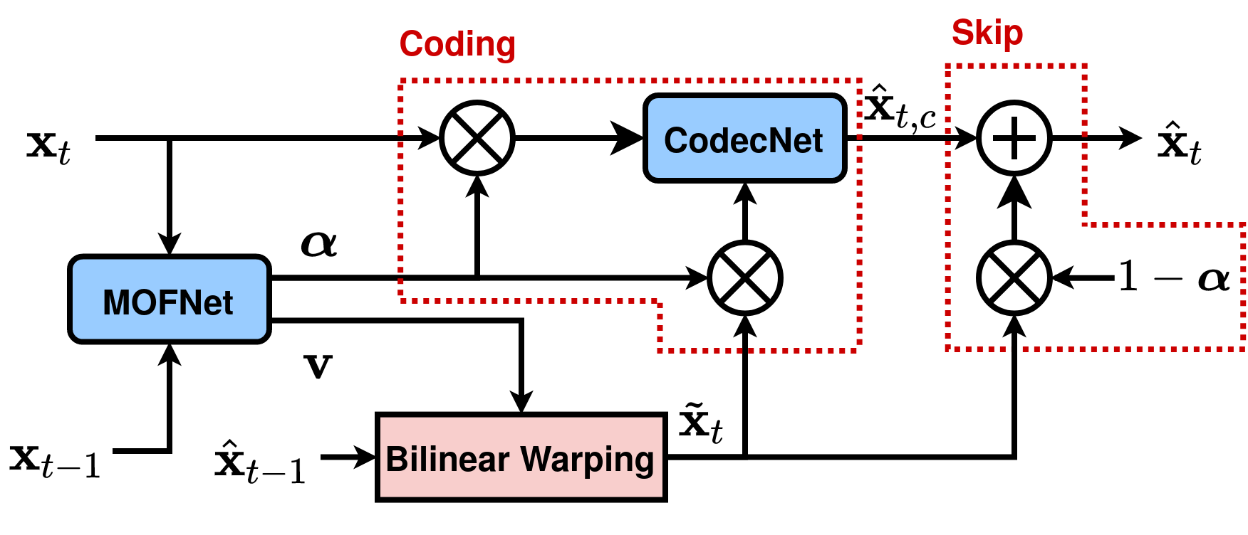
This section details the main components of the proposed coding scheme, presented in Fig. 1.

III-A MOFNet: Mode Selection and Optical Flow Estimation
Performing a proper prediction of the current frame is an essential element of video coding systems. Indeed, most parts of the frame can be recovered from already received frames using motion vectors transmitted at low rate.
In this work, a dense optical flow is used to represent the 2-D motion of each pixel between and . The estimated optical flow is used to perform the prediction:
| (2) |
where is a bilinear warping, as illustrated in Fig. 1.
The proposed coding scheme splits into two complementary pixels sets and , corresponding to two coding modes. The pixels in are directly copied from the prediction as Skip Mode in classical codecs. Those in are transmitted by an autoencoder. The presence of two competiting coding modes allows to select the most suited one for each pixel, resulting in better RD performances. However, this partitioning into two sets is not straightforward, as the rate and the distortion of a pixel depends on the coding choice made for both previous and future pixels.
A single network MOFNet is proposed, to compute and convey the coding mode selection and the flow estimation. MOFNet is defined as a function :
| (3) |
where is the pixel-wise weighting matrix, the optical flow and the associated rate. The pixel-wise weighting matrix is real-valued such that smooth transitions between coding modes are possible, avoiding blocking artifacts.
III-B CodecNet
An immediate way of using the prediction is to perform residual coding i.e. coding only the prediction error . Albeit widely used in legacy video coding systems, this method is not the best option for leveraging information from . Indeed, from a source coding perspective:
| (4) |
where denotes the Shannon entropy. Therefore coding while retrieving all information from can result in less information to transmit than residual coding.
In this work, an autoencoder CodecNet is used to transmit , selected by the pixel-wise weighting matrix . CodecNet learns the appropriate mixture of and for both the encoder and the decoder, resulting in potentially better coding performances than direct residual coding. In contrast with residual coding, the processing performed by CodecNet is denoted as conditional coding in the remaining of the paper. CodecNet is defined as a function , coding using information from :
| (5) |
where element-wise matrix multiplication is denoted by , is the reconstruction of and the associated rate. The same is used for all color channels.
III-C Complete System
One of MOFNet purposes is to split transmission between CodecNet and skip mode. Thus the complete reconstruction is:
| (6) |
This equation highlights that the role of is to zero areas from before coding them with CodecNet, in order to save their associated rate. Figures 3(c), 3(e) and 3(g) illustrate that CodecNet does not allocate bits to areas zeroed by . MOFNet and CodecNet are trained in an end-to-end fashion to minimize the rate-distortion trade-off:
| (7) |


IV Practical Implementation
IV-A Networks Architecture
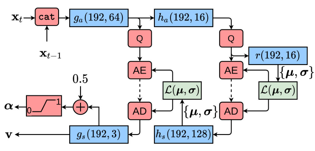
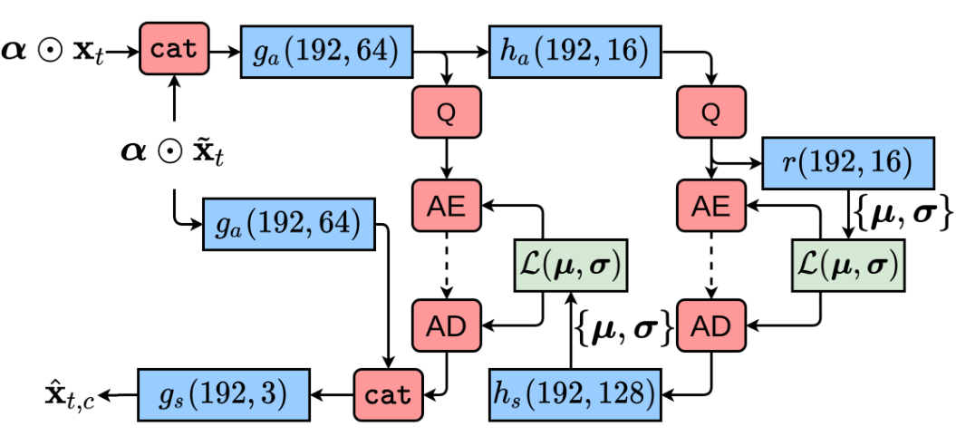
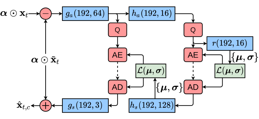
The two neural networks proposed in section III, MOFNet and CodecNet, are described in Fig. 2. They are both based on the common autoencoder with hyperprior (AE-HP) architecture [15] used in previous learned image coding systems.
MOFNet role is to compute and convey the optical flow and the pixel-wise weighting . Authors in [5] show that a single network can perform both estimation and coding of . This work follows this method and uses a common learned image coding architecture, depicted in Fig. 2(b). MOFNet takes and as inputs and retrieves and at the decoder side. To ensure that remains in , a clipping function is used. A bias of is added before clipping as it empirically ensures better convergence.
The purpose of CodecNet is to transmit pixels of conditioned to its prediction . It is designed as an AE-HP system with the ability to learn an arbitrary complex mixture of and , at the encoder side and the decoder side. CodecNet architecture (see Fig. 2(c)) is a direct extension of image coding autoencoders with both the frame and its prediction as inputs. Therefore, the encoder is able to learn a non-linear mixture of and . The same principle is used for the decoder, which has the latents from and as input, allowing it to invert the transform performed by the encoder.
IV-B Training
All networks are trained in an end-to-end fashion to minimize the global loss function stated in eq. (7). Non-differentiable parts are approximated as in Ballé’s work [13, 15] to make the training possible.
To the best of our knowledge, all previous work learn the flow with either a pre-trained network and/or a dedicated loss term. In the proposed coding scheme, the optical flow can be learned without a seperately pre-trained network or a dedicated additional loss term. Indeed, the areas directly copied from heavily foster the learning of a proper flow, with no need of pre-training and/or a dedicated loss term.
However, due to the competition between signal paths, some care is taken when training. The training process is composed of three phases:
- 1.
During the first five epochs, skip mode and CodecNet are not ready to compete. Thus, is frozen and set to 1 for one half of the frame, 0 for the other half. This allows to learn a meaningful MOFNet and CodecNet without interference between them.
- 2.
Alternate training of MOFNet and CodecNet, one epoch for each (i.e. the other network weights are frozen) for 45 epochs.
- 3.
Joint training of MOFNet and CodecNet for 20 epochs.
Training is performed on the CLIC20 P-frame dataset [11]. The training set is composed of half a million pairs of crops, randomly extracted from consecutive frames. The same learning rate of is used for all three phases with a decrease down to during the final phase.
V System Behavior and Visualisation
The processing of a pair of frames is thoroughly described in this section, illustrated in Fig. 3. The example frames are extracted from the CLIC20 P-frame dataset, sequence Vlog_2160P-310b frames 36 and 37.
First, MOFNet takes and (shown in Fig. 3(a)) as inputs. The pair of frames are encoded and decoded as and . The optical flow (illustrated in Fig. 3(d)) is used to perform a prediction of through a bilinear warping. Then, the pixel-wise weighting (see Fig. 3(c)) arbitrates between skip mode and CodecNet. Fig. 3(e) and 3(f) present the areas selected for both coding modes11 1 As images are in YCbCr format, zeroed areas appear in green. Finally, the two coding modes are combined to obtain the reconstructed frame, shown in Fig. 3(b).
represent areas in more suited for skip mode than coding, i.e. areas which are either well handled by motion compensation or too costly to transmit. In order to select these areas for skip mode, tends to be zero for pixels in . These areas correspond to the green ones in Fig. 3(e), e.g. the grass and most of the man. By contrast, is close to one for pixels in , which are not well predicted enough or relatively easy to transmit. To achieve an acceptable quality, those pixels rely on transmission by CodecNet. These areas appear in green in Fig. 3(f). They correspond to contents which are difficult to predict such as the edges of the man or the leaves of the tree.
Figures 3(g) and 3(h) represent the spatial distribution of the rate of CodecNet and ModeNet. As expected from eq. (6), areas with a small are zeroed before CodecNet and thus transmitted for free. The motion and the partitioning conveyed by MOFNet is complex throughout the frame, resulting in a small rate almost evenly distributed spatially.
This illustration highlights that MOFNet is able to learn a complex optical field, e.g. modeling a rotation motion for the background while not including the man in the foreground. In the meantime, MOFNet is also able to learn , an accurate and smooth partitioning of the frame, which indicates the properly predicted areas and those needing to rely on CodecNet. Both and are conveyed at low-bitrate (around 0.02 bpp in this example).
VI Experimental Results
VI-A System Performance
The performance of the proposed inter frame coding scheme is assessed on the CLIC20 validation set, under the challenge test conditions. In order to obtain a RD-curve, the system is trained with different . The rate-distortion curves are shown Fig. 4.
The proposed method is evaluated against the state-of-the-art video coder HEVC in low-delay P (LDP) coding configuration. HEVC encodings are performed with the HM 16.20 reference software slightly modified to be aligned with CLIC20 test conditions where the reference frame is lossless. Our approach performs as good as HEVC, proving the relevance of the proposed method. This demonstrates that the optical flow learned in an end-to-end fashion, without pre-training or a dedicated loss term, is able to achieve a temporal prediction competitive with state-of-the-art motion compensation.
VI-B Ablation study
The benefits of each component of the proposed system is also assessed in Fig. 4. In order to estimate the rate saving offered by the different components, the BD-rate [16] metric is used. It represents the rate difference necessary to obtain identical quality between two systems.
The interest of performing a conditional coding of and instead of residual coding is evaluated by training a complete systems (i.e. including skip mode) while substituting CodecNet by a neural-based residual codec, detailed in Fig. 2(d). Its performance is presented on Fig. 4 as Residual + Skip. According to the BD-rate metric, conditional coding reduces the rate by 32 % compared to direct residual coding, highlighting its relevance.
The improvements brought by the competition between skip mode and CodecNet is evaluated by setting (CodecNet only) or (Skip only) configuration. Both configurations are re-trained starting from the complete system and result in a performance decrease. In Skip only configuration, the system output is directly the prediction . Since prediction can not explain all the frame to code the performance saturates at low quality. In CodecNet only configuration, the absence of competition between coding modes results in a rate increase of 53 % according to the BD-rate metric. This experiment demonstrates the benefit of using a competition between skip mode and CodecNet.
VII Conclusions
In this paper, a new method for inter frame coding is introduced, based on two autoencoders: MOFNet and CodecNet. MOFNet role is to compute and convey the optical flow and a pixel-wise mode selection, allowing to choose between skip mode and coding through CodecNet.
The proposed coding scheme performances are illustrated under the CLIC20 P-frame coding task and it is shown to be competitive HEVC. Moreover, skip mode enables to learn the optical flow in an actual end-to-end fashion i.e. with no need of a pre-training or a dedicated loss term.
In future work, we plan to adapt the proposed coding scheme to more complex video coding tasks such as coding frames with multiple references, both in the past and in the future. This implies to enhance all sub-networks to leverage as much information as possible from the references.
References
- [1] D. Marpe, T. Wiegand, and G. J. Sullivan, “The H.264/MPEG4 advanced video coding standard and its applications,” IEEE Communications Magazine, vol. 44, no. 8, pp. 134–143, 2006. [Online]. Available: https://doi.org/10.1109/MCOM.2006.1678121
- [2] G. J. Sullivan, J.-R. Ohm, W.-J. Han, and T. Wiegand, “Overview of the high efficiency video coding (hevc) standard,” IEEE Trans. Cir. and Sys. for Video Technol., vol. 22, no. 12, pp. 1649–1668, Dec. 2012. [Online]. Available: http://dx.doi.org/10.1109/TCSVT.2012.2221191
- [3] S. K. J. Chen, Y. Ye, “Algorithm description for versatile video coding and test model 8 (vtm 8),” Jan. 2020.
- [4] G. Lu, W. Ouyang, D. Xu, X. Zhang, C. Cai, and Z. Gao, “DVC: an end-to-end deep video compression framework,” in IEEE Conference on Computer Vision and Pattern Recognition, CVPR 2019, Long Beach, CA, USA, pp. 11 006–11 015. [Online]. Available: http://openaccess.thecvf.com/content_CVPR_2019/html/Lu_DVC_An_End-To-End_Deep_Video_Compression_Framework_CVPR_2019_paper.html
- [5] H. Liu, H. Shen, L. Huang, M. Lu, T. Chen, and Z. Ma, “Learned video compression via joint spatial-temporal correlation exploration,” CoRR, vol. abs/1912.06348, 2019. [Online]. Available: http://arxiv.org/abs/1912.06348
- [6] A. Djelouah, J. Campos, S. Schaub-Meyer, and C. Schroers, “Neural inter-frame compression for video coding,” in The IEEE International Conference on Computer Vision (ICCV), October 2019.
- [7] R. Yang, F. Mentzer, L. V. Gool, and R. Timofte, “Learning for video compression with hierarchical quality and recurrent enhancement,” CoRR, vol. abs/2003.01966, 2020. [Online]. Available: https://arxiv.org/abs/2003.01966
- [8] A. Ranjan and M. J. Black, “Optical flow estimation using a spatial pyramid network,” CoRR, vol. abs/1611.00850, 2016. [Online]. Available: http://arxiv.org/abs/1611.00850
- [9] D. Sun, X. Yang, M. Liu, and J. Kautz, “Pwc-net: Cnns for optical flow using pyramid, warping, and cost volume,” in IEEE Conference on Computer Vision and Pattern Recognition, CVPR 2018, Salt Lake City, UT, USA, 2018, pp. 8934–8943. [Online]. Available: http://openaccess.thecvf.com/content_cvpr_2018/html/Sun_PWC-Net_CNNs_for_CVPR_2018_paper.html
- [10] A. Golinski, R. Pourreza, Y. Yang, G. Sautière, and T. S. Cohen, “Feedback recurrent autoencoder for video compression,” CoRR, vol. abs/2004.04342, 2020. [Online]. Available: https://arxiv.org/abs/2004.04342
- [11] Workshop and C. on Learned Image Compression, “https://www.compression.cc/,” June 2020.
- [12] Z. Wang, E. P. Simoncelli, and A. C. Bovik, “Multi-scale structural similarity for image quality assessment,” in in Proc. IEEE Conf. on Signals, Systems, and Computers, 2003, pp. 1398–1402.
- [13] J. Ballé, V. Laparra, and E. P. Simoncelli, “End-to-end optimized image compression,” in 5th International Conference on Learning Representations, ICLR 2017, Toulon, France, 2017. [Online]. Available: https://openreview.net/forum?id=rJxdQ3jeg
- [14] D. Minnen, J. Ballé, and G. Toderici, “Joint autoregressive and hierarchical priors for learned image compression,” in Conference on Neural Information Processing Systems 2018, NeurIPS,, Montréal, Canada., pp. 10 794–10 803. [Online]. Available: http://papers.nips.cc/paper/8275-joint-autoregressive-and-hierarchical-priors-for-learned-image-compression
- [15] J. Ballé, D. Minnen, S. Singh, S. J. Hwang, and N. Johnston, “Variational image compression with a scale hyperprior,” in 6th International Conference on Learning Representations, ICLR 2018, Vancouver, BC, Canada, 2018. [Online]. Available: https://openreview.net/forum?id=rkcQFMZRb
- [16] G. Bjontegaard, “Calculation of average psnr differences between rd-curves,” in ITU-T Q.6/16, Doc. VCEG-M33, March 2001.