UBER-GNN: A User-Based Embeddings Recommendation based on Graph Neural Networks Conference: Workshop; ;
Abstract.
The problem of session-based recommendation aims to predict user next actions based on session histories. Previous methods models session histories into sequences and estimate user latent features by RNN and GNN methods to make recommendations. However under massive-scale and complicated financial recommendation scenarios with both virtual and real commodities , such methods are not sufficient to represent accurate user latent features and neglect the long-term characteristics of users.
To take long-term preference and dynamic interests into account, we propose a novel method, i.e. User-Based Embeddings Recommendation with Graph Neural Network, UBER-GNN for brevity. UBER-GNN takes advantage of structured data to generate long-term user preferences, and transfers session sequences into graphs to generate graph-based dynamic interests. The final user latent feature is then represented as the composition of the long-term preferences and the dynamic interests using attention mechanism.
Extensive experiments conducted on real Ping An scenario show that UBER-GNN outperforms the state-of-the-art session-based recommendation methods.
Keywords:
Recommender Systems, Graph Representation Learning, Deep Learning1. Introduction

In financial service category, Ping An Jinguanjia, JD Finance, Ant Fortune (Ant Financial) are top 3 applications on Mobile. As a comprehensive app ensembles diverse functions such as insurance purchases, investment services, Health consulting and so on, Jinguanjia also provides a typical E-Commerce platform for online shopping, serving over 15,000,000 users per month.
Besides Jinguanjia, with the high-speed development of China’s Mobile Internet, more and more online transactions are driven by intelligent and efficient recommender algorithms. E-Commerce platforms like Alibaba, searching and advertising platforms like Baidu, and O2O lifestyle service platforms like Meituan, have their our recommender algorithm systems based on methods like association rules, Machine Learning(eg. collaborative filtering). Moreover, with the rapid improvement of computers in recent years, algorithms like DNNs have made breakthroughs in aspects like Computer Visions and others, more and more domestic E-Commerce and advertising platforms have been contributing new explorations and innovations. For instance, In (Cheng et al. 2016), members from Google Group explored a novel recommendation framework called Wide&Deep for jointly training feed-forward neural networks with embedding and linear model with feature transformations; In(Wang et al. 2019) , Meituan-Dianping Group advocated a Multi-task feature learning approach for knowledge graph enhanced recommendation, which presented a end-to-end deep KG network; In (Zhou et al. 2017), the group from Alibaba Group proposed a novel recommendation framework through attention-based DNN in consist of the heterogeneous behaviors of users.
Nevertheless, Deep Learning framework is not effective enough on the E-Commerce platform of Jinguanjia, where users can select various items more than hundred thousands types, including virtual financial commodities like short-term medical insurance, physical examination services, and real commodities like fruits, snacks, etc. Considering the mixture recommendation with virtual and real commodities, different from traditional E-Commerce only with real commodities, it is more complicated to predict the next-purchase item of users. During the practice, the prediction methods of CTR (click-through rate) like DeepFM (Guo et al. 2017), which combines FM (factorization machines) and deep learning architecture, play not well, since they solely extracts implicit interactions of short-term behaviors of users without aware of the purchase sequences and the relations of items. On the other hand, unlike shopping fruits or snacks, users are acting much more reasonably and making decision much more cautiously when selecting a financial commodity. Therefore, the traditional session-based recommendation methods like newest one SR-GNN(Wu et al. 2018), have limitations as only using item-purchased sessions but ignoring the characteristics of users.
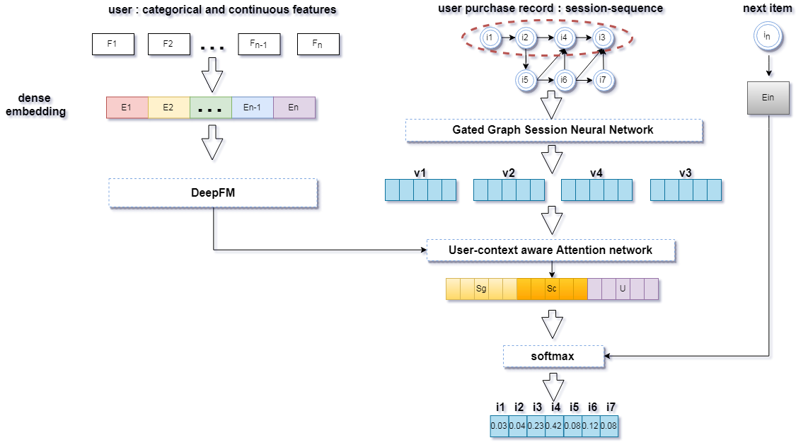
As a consequence, we propose a novel recommendation architecture on session-based Graph Neural Network, with the enhancement of learning sophisticated features embeddings of users through DeepFM method as shown in Figure 1.
The main contributions of our works include:
- •
We propose a novel session-based recommendation architecture to solve the massive-scale and complicated recommendation scenario with both virtual and real commodities.
- •
Our method takes advantages of latent user embeddings and graph-based latent item embeddings, to make an impressive progress on prediction of next-purchase commodity.
- •
Through the off-line experiments on the real transactions dataset of Jinguanjia, our model has shown improvement on precision and MRR than other state-of-the-art models. Additionally, we have completed the low stream test in the live environment and achieved advance than previous methods.
2. problem formulation
In session-based recommendation scenario, the main target is to predict which item will purchase next. Here is the formulation of this problem as below:
stands for a purchase session sequence, ordered by timestamps. stands for all unique items involved in all the purchase sessions. The target of recommendation is to predict the next purchase item in . In addition, we collect the portraits dataset of users in session sequences, such as characteristics of population, financial behavior, consumption behavior and so on. For each user, to judge a session-based recommendation model, for each session , the model generates probability vector for all items in , and each value of is the recommendation score of the corresponding item. Thus, the top-K recommendation will select K items from correspondingly.
3. proposed method
In this section, we illustrate our method named UBER-GNN (user-based embeddings recommendation on Graph Neural Networks), as shown in Figure 2. At first, we explain the vital step how user-based embeddings are generated. Second, in SECTION 3.2 and 3.3, we construct a GNN from purchase-sessions. Third, we describe the combinations of user embeddings and session embeddings of items. Finally, we present the details of model training.
3.1. User context based embeddings
In this section, we explain the extraction user-context based embeddings from the portraits data of users. Inspired by the end-to-end method DeepFM(Guo et al. 2017), we carry out low-order (order-2) feature interactions from Factorization Machines and high-order (above order-3) from DNN. The portraits data of users includes categorical and continuous features. To construct features embeddings, initially each categorical one is represented as a vector of one-hot encoding, and each continuous one is represented as a vector of one-hot encoding after discretization. we regard as the input of DeepFM, where X is a -dimensional vector, with being the vector of i-th field and n is the number of fields. After fed into DeepFM, we can generate user embeddings like:
| (1) |
where is the output of FM part and is the output of DNN part. is a sigmoid function.
3.1.1. FM part
The FM part is a factorization machine, which can learn order-1 by addition way and order-2 by inner product way of feature interactions, shown as:
| (2) |
where is the linear transformation of and the other part reflects the order-2 transformation. , are latent vectors.
3.1.2. DNN part
The DNN part is a feed-forward neural network, which can learn high-order feature interactions. =X is input into DNN and for each layer:
| (3) |
where i is the layer depth and is an activation function. ,, are the output of previous layer, weight and bias of the layer . Thus , where is the number of hidden layers of DNN.
3.2. Session graph representation
In this section, we introduce a method to represent graph. For each session sequence , there is a directed graph structure , where nodes collection takes each node , edges collection takes each in session sequence . stands for a user purchase after in the session . Because some items may be purchased more than once in a session , we assign each edge with a normalized weight, which is calculated as the occurrence of the edge divided by the outdegree of the start node of the edge.
Besides, the connection matrix is introduced to represents a session graph with an unique structure. , which represents weighted connections of outgoing and incoming edges in the session graph respectively. For example, a session graph and the connection matrix is shown in Figure 3, and the corresponding session is having nodes and purchased over once.
Meanwhile, our model will transform every item into a same embedding space with a node vector which is a latent vector learned via graph neural network(GNN). Additionally, each session can be represented by an embedding vector s at SECTION 3.4, which is combined through the node vectors v generated from GNN.
3.3. Item embeddings via GNN

Thirdly, The plain vanilla GNN is proposed by (Scarselli et al. 2009), then (Li et al. 2016) improved GNN by replacing propagation model with gated recurrent units(GRUs) and proposed Gated graphed Sequence Neural Networks(GGS-NNs) with Back-Propagation Through Time(BPTT) to compute gradients. Furthermore, GGS-NNs works are very suitable for session-based recommendation problems, as it can automatically extract features of session graphs with consideration of nodes having many connections.
In addition, there is an analogy can be drawn between the adaptation from GNNs to GGS-NNs, and the adaptation from LSTMs(Hochreiter and Schmidhuber 1997) to GRUs(Chung et al. 2014) in Recursive Neural Networks (Socher et al. 2011). In GGS-NNs, instead of the standard GNN recurrence, new adaptation can improve the long-term propagation of information across a graph structure.
In the GRU of GGS-NNs, the gated structure is shown like below:
| (4) |
| (5) |
| (6) |
| (7) |
| (8) |
Where and are the update gate and reset gate, and are the activation and the candidate activation. In equation(4), is the concatenation of two columns of in ; is the list of node vectors in session and represents the total number of total nodes in ; and are hyper-parameters matrices where d is pre-set as the dimension of item embeddings . In equation (5) and (6), operator is the sigmoid function, and are hyper-parameters matrices. In equation (7) and (8), operator is the element-wise multiplication operator and are hyper-parameters matrices.
To better illustrate, here we explain how GRU generate vector of item embeddings. GGS-NN can proceed nodes of session graph at the same time. In each GRU, equation (4) is used for information propagation between different nodes of the session graph construction of . Specifically, at first,the GRU extracts the latent vectors of neighborhoods and feeds them as input into the neighbor GRUs. Second, the update gate of equation (5) and reset gate of equation (6), utilize the sigmoid function to decide what information to be preserved or discarded respectively. Third, equation (7) constructs the candidate state by the current state, the reset gate and the previous gate. Finally, the final state of equation (8) is the combination of the previous state and the candidate state, with the consideration of the update gate. As a consequence, after all nodes in session graphs is processed by GGS-NN until convergence, we can obtain the final node vectors of all item embeddings.
3.4. Session embeddings with attention to user context
Regardless of user static features, previous session-based recommendation methods only focus on session sequences. On the contrary, to better predict the user’s next purchase item, we address an attention mechanism to combine users context as user embedding vectors and purchase sessions as item embedding vectors. In this section, we illustrate how to enhance session-based method with attention to user context.
| (9) |
| (10) |
where is the output from SECTION 3.1 which is unique for each user. , ,, as hyper-parameters, control the weights of embeddings. In SECTION 3.3, we generate the vectors of all nodes after feed all session graphs into GGS-NNs. Then in equation (10), instead of using to represent user purchase session , we extract essential latent information as by aggregating all nodes vectors. Moreover, to consider the influence of last-time purchase, we assign . therefore, we apply a hybrid combination through the concatenation of current purchase interest, global purchase preference and user’s latent context.
| (11) |
where matrix compresses three embedding vectors into latent space .
Furthermore, to emphasize the effect of different attention approaches, we assign adaptation to .
(1) global embedding with average pooling, equation (10) is changed as:
| (12) |
(2) global embedding with attention mechanism that only considers local embedding, equation (9) is changed as:
| (13) |
(3) global embedding with attention mechanism that only considers user embedding, equation (9) is changed as:
| (14) |
All the details of comparison is evaluated in SECTION 4.5.
3.5. Model training
With the compression process, we obtain each session latent vector, then we can compute the recommended score-value for each purchase item by times item vector and session vector , which is defined as:
| (15) |
Then the score vector where N stands for the total number of items is fed into softmax function to get the output probabilities:
| (16) |
where denotes the probability of items which is the next purchase one in session .
Finally, we take cross-entropy as the loss function of the prediction and the ground truth for each session . It is shown as:
| (17) |
Accordingly, to train the whole model, we use the Back-Propagation Through Time(BPTT) algorithm.
4. Experimental result
4.1. Datasets description
| Dataset | financial-include | financial-exclude |
|---|---|---|
| # of commodities | 82,126 | 65,623 |
| # of users | 24,022 | 21,921 |
| # of transactions | 753,960 | 473,495 |
| # of sessions | 91,433 | 76,816 |
| Avg length of session | 8.246 | 6.164 |
We implement and evaluate our method on real-world transaction data of Ping An Jinguanjia, which owns sufficient, multidimensional portraits of users to generate precise and comprehensive embeddings of user features.
Datasets have two major parts; First is the portraits data of users, including 306 features (212 categorical ones and 94 continuous ones); Second is the purchase session data of users, within 12 months selected from March 2018 to March 2019. Besides, to fair compare, we extract sessions data of length 1 and filter out items appearing 5 times from the initial datasets. And to generate the labels, we split the purchase sessions. For example, a purchase session can be extracted sequences and labels like, ,, …, , where is next-purchase item. Furthermore, considering Jinguanjia as a complex E-Commerce platform supplies not only real commodities but also virtual financial commodities, we select sessions without financial commodities as financial-exclude dataset.
The statistics of datasets are summarized in Table 1.
4.2. Baseline methods
For better comparison, we choose baseline methods as follows:
- •
BPR: (Rendle et al. 2010)optimized a pairwise ranking objective function via stochastic gradient descent. - •
DeepFM: (Guo et al. 2017) combined FM and deep learning architecture to learn implicit user behaviors for CTR prediction. - •
GRU4REC:(Hidasi et al. 2016) used RNNs to model user sequences for the session-based recommendation. - •
SRGNN:(Wu et al. 2018) used GNNs to model session sequences as graph structured data.
4.3. Evaluation Metrics
P@20(Precision) stands for the proportion of correctly recommended items among the top-20 items.
MRR@20(Mean Reciprocal Rank) stands for a statistic measure for evaluating average accuracy of ranking in top-20. The query of a reciprocal rank of top-20 is the multiplicative inverse of the rank of the first correct answer: 1 for first place, 12 for second place, 13 for third place and 0 for exceeding top-20.
4.4. Parameters settings
In our experiments, validation set is a random 20 percent subset of the training set. All parameters are initialized using a Gaussian distribution with a mean of zero and standard deviation of 0.1. In our methods, we set the hyper-parameters as following: the hidden size and the batch size is set to 200 and 32 respectively. The mini-batch Adam optimizer is utilized to optimize parameters, where the initial learning rate is set to 0.1 and will exponential decay to 0.01 after every 10 epoches. Moreover, the L2 penalty is set to 1e-5 to get better performance.
4.5. Results analysis
Comparison with baseline methods:
In order to evaluate the overall performance of our proposed model, we compare it with other state-of-art session-based recommendation methods and classical CTR prediction method DeepFM. The overall performance in terms of P@20 and MRR@20 is shown in Table 2.
In our proposed UBER-GNN model, it jointly utilizes both graph-structure data aggregated by session sequences and user-based classical-structure data. Thus our model consider user long-term static latent characteristics and preferences as well as their dynamic latent interests. According to the experiments, our proposed UBER-GNN model achieves the best performance on both two datasets in terms of Precision@20 and MRR@20.
Regarding traditional algorithms like BPR,the performance is relatively poor. Such simple methods make recommendations solely based on history items, which is problematic in session-based recommendation scenarios. As well as DeepFM, it’s not suitable when predicting next-purchase. Likewise, Short/Long-term memory models, like GRU4REC, use recurrent units to capture a user’s global interest. Such method explicitly model the user’s global behavior preferences. While graph neural network based models, like SR-GNN, transfer session history sequences into graph-structured data and utilize gated graph neural network to update item embeddings. However, their performances are still inferior to that of our proposed UBER-GNN Model.
Compared with the state-of-art models like SR-GNN and GRU4REC, our model firstly considers user-based classical-structure data to better represent user long-term latent characteristics and preferences, and further models transitions between items into graph that can capture more complex and implicit connections between recent behaviors. Whereas in GRU4REC and SR-GNN, they explicitly model item history and obtain user representations through sequences, losing sight of the characteristics information of users.
| Method | financial-include | financial-exclude | ||
|---|---|---|---|---|
| P@20(%) | MRR@20(%) | P@20(%) | MRR@20(%) | |
| BPR | 51.43 | 12.48 | 53.77 | 13.24 |
| DeepFM | 65.03 | 14.41 | 63.89 | 13.75 |
| GRU4REC | 68.48 | 20.09 | 65.59 | 18.84 |
| SRGNN | 74.64 | 24.47 | 75.62 | 25.01 |
| Ours | 77.91 | 26.66 | 78.04 | 25.75 |
Comparison with variants on session embedding strategy:
We compare the session embedding strategy with following different attention approaches:
(1) global embedding with average pooling.
(2) global embedding with attention mechanism that only considers local embedding.
(3) global embedding with attention mechanism that only considers user embedding.
(4) global embedding with attention mechanism that both considers user embedding and local embedding.
The result of methods with four different strategies on both two datasets are given in Table 3.
Firstly, the result is shown that attention mechanisms are useful in extracting significant behaviors from history sequences. Average pooling strategy may not be adaptive for the sequence scenario due to uncertain noisy behaviors.
Furthermore, hybrid attention embedding strategy considering both static user embedding and dynamic local embedding achieves best results on both two datasets. It validates the importance of explicitly incorporating dynamic latent features and static latent features. In additional, it supports that both static user features and dynamic local features are crucial for session-based recommendation.
| Method | financial-include | financial-exclude | ||
|---|---|---|---|---|
| P@20(%) | MRR@20(%) | P@20(%) | MRR@20(%) | |
| V1 | 75.21 | 24.92 | 75.42 | 24.98 |
| V2 | 77.01 | 26.22 | 75.83 | 25.34 |
| V3 | 76.59 | 25.87 | 77.05 | 25.56 |
| V4 | 77.91 | 26.66 | 78.04 | 25.75 |
5. Conclusions
In this paper, we propose a novel architecture for session-based recommendation that takes long-term preference and dynamic interests into consideration. The proposed method UBER-GNN not only takes advantage of structured data to generate long-term user preferences, but also transfers session sequences into graphs to generate graph-based dynamic interests. In addition, it develops an attention strategy to ensemble long-term preferences and dynamic interests to better predict users’ next actions. Extensive experiments conducted on real Ping An scenario show that UBER-GNN outperforms the state-of-the-art session-based recommendation methods.
References
- (1)
- Cheng et al. (2016) Heng-Tze Cheng, Levent Koc, Jeremiah Harmsen, Tal Shaked, Tushar Chandra, Hrishi Aradhye, Glen Anderson, Greg Corrado, Wei Chai, Mustafa Ispir, Rohan Anil, Zakaria Haque, Lichan Hong, Vihan Jain, Xiaobing Liu, and Hemal Shah. 2016. Wide & Deep Learning for Recommender Systems. CoRR abs/1606.07792 (2016). arXiv:1606.07792 http://arxiv.org/abs/1606.07792
- Chung et al. (2014) Junyoung Chung, Çaglar Gülçehre, KyungHyun Cho, and Yoshua Bengio. 2014. Empirical Evaluation of Gated Recurrent Neural Networks on Sequence Modeling. CoRR abs/1412.3555 (2014). arXiv:1412.3555 http://arxiv.org/abs/1412.3555
- Guo et al. (2017) Huifeng Guo, Ruiming Tang, Yunming Ye, Zhenguo Li, and Xiuqiang He. 2017. DeepFM: A Factorization-Machine based Neural Network for CTR Prediction. CoRR abs/1703.04247 (2017). arXiv:1703.04247 http://arxiv.org/abs/1703.04247
- Hidasi et al. (2016) Balázs Hidasi, Alexandros Karatzoglou, Linas Baltrunas, and Domonkos Tikk. 2016. Session-based Recommendations with Recurrent Neural Networks. In 4th International Conference on Learning Representations, ICLR 2016, San Juan, Puerto Rico, May 2-4, 2016, Conference Track Proceedings. http://arxiv.org/abs/1511.06939
- Hochreiter and Schmidhuber (1997) Sepp Hochreiter and Jürgen Schmidhuber. 1997. Long Short-Term Memory. Neural Comput. 9, 8 (Nov. 1997), 1735–1780. DOI:http://dx.doi.org/10.1162/neco.1997.9.8.1735
- Li et al. (2016) Yujia Li, Daniel Tarlow, Marc Brockschmidt, and Richard Zemel. 2016. Gated Graph Sequence Neural Networks. ICLR abs/1511.05493 (2016). arXiv:1511.05493 https://arxiv.org/abs/1511.05493
- Rendle et al. (2010) Steffen Rendle, Christoph Freudenthaler, and Lars Schmidt-Thieme. 2010. Factorizing Personalized Markov Chains for Next-basket Recommendation. In Proceedings of the 19th International Conference on World Wide Web (WWW ’10). ACM, New York, NY, USA, 811–820. DOI:http://dx.doi.org/10.1145/1772690.1772773
- Scarselli et al. (2009) Franco Scarselli, Marco Gori, Ah Chung Tsoi, Markus Hagenbuchner, and Gabriele Monfardini. 2009. The Graph Neural Network Model. IEEE transactions on neural networks / a publication of the IEEE Neural Networks Council 20 (01 2009), 61–80. DOI:http://dx.doi.org/10.1109/TNN.2008.2005605
- Socher et al. (2011) Richard Socher, Cliff C. Lin, Andrew Y. Ng, and Christopher D. Manning. 2011. Parsing Natural Scenes and Natural Language with Recursive Neural Networks. In Proceedings of the 26th International Conference on Machine Learning (ICML).
- Wang et al. (2019) Hongwei Wang, Fuzheng Zhang, Miao Zhao, Wenjie Li, Xing Xie, and Minyi Guo. 2019. Multi-Task Feature Learning for Knowledge Graph Enhanced Recommendation. CoRR abs/1901.08907 (2019). arXiv:1901.08907 http://arxiv.org/abs/1901.08907
- Wu et al. (2018) Shu Wu, Yuyuan Tang, Yanqiao Zhu, Liang Wang, Xing Xie, and Tieniu Tan. 2018. Session-based Recommendation with Graph Neural Networks. CoRR abs/1811.00855 (2018). arXiv:1811.00855 http://arxiv.org/abs/1811.00855
- Zhou et al. (2017) Chang Zhou, Jinze Bai, Junshuai Song, Xiaofei Liu, Zhengchao Zhao, Xiusi Chen, and Jun Gao. 2017. ATRank: An Attention-Based User Behavior Modeling Framework for Recommendation. CoRR abs/1711.06632 (2017). arXiv:1711.06632 http://arxiv.org/abs/1711.06632