跳到论文正文
W Papers独立论文阅读器 arXiv:2008.02418 论文正文 计算阅读时间 · 0%
引用这篇论文根据当前论文元数据生成,正式投稿前建议核对。


License: arXiv.org perpetual non-exclusive license
arXiv:2008.02418v3 [math.OC] 31 May 2021

Finding Equilibria in the Traffic Assignment Problem with Primal-Dual Gradient Methods for Stable Dynamics Model and Beckmann Model

Meruza Kubentayeva Affiliation: Institute for Information Transmission Problems RAS, kubentay@gmail.com    Alexander Gasnikov Affiliation: Moscow Institute of Physics and Technology, Affiliation: Institute for Information Transmission Problems RAS, Affiliation: Higher School of Economics, gasnikov@yandex.ru
Abstract

In this paper we consider the application of several gradient methods to the traffic assignment problem: we search equilibria in the stable dynamics model (Nesterov and De Palma 2003) and the Beckmann model. Unlike the celebrated Frank–Wolfe algorithm widely used for the Beckmann model, these gradients methods solve the dual problem and then reconstruct a solution to the primal one. We deal with the universal gradient method, the universal method of similar triangles, and the method of weighted dual averages, and estimate their complexity for the problem. Due to the primal-dual nature of these methods, we use a duality gap in a stopping criterion. In particular, we present a novel way to reconstruct admissible flows in the stable dynamics model, which provides us with a computable duality gap.

Keywords: stable dynamics model, Beckmann model, traffic equilibrium, universal gradient method, universal method of similar triangles, method of weighted dual averages, duality gap

1 Introduction

The Beckmann model for searching static traffic equilibria in road networks is among the most widely used models by transportation planners (Beckmann et al. 1956; Patriksson 2015). The equilibria found are practical for evaluating the network efficiency and distribution of business centers and residential areas, and establishing urban development plans, etc. This model introduces a cost function on every link of a transportation network, which defines a dependence of the travel cost on the flow along the link. In practice the BPR functions are usually employed (US Bureau of Public Roads 1964):

τe​(fe)=t¯e​(1+ρ​(fef¯e)1μ),\tau_{e}(f_{e})=\bar{t}_{e}\left(1+\rho\left(\frac{f_{e}}{\bar{f}_{e}}\right)^{\frac{1}{\mu}}\right), (1)

where t¯e\bar{t}_{e} are free flow times, and f¯e\bar{f}_{e} are road capacities of a given network’s link ee. We take these functions with parameters ρ=0.15\rho=0.15 and μ=0.25\mu=0.25.

Nesterov and De Palma 2003 proposed an alternative model called the stable dynamics model, which takes an intermediate place between static and dynamic network assignment models. Namely, its equilibrium can be interpreted as the stationary regime of some dynamic process. Its key assumption is that we no longer introduce a complex dependence of the travel cost on the flow (as in the standard static models), but only pose capacity constraints, i.e. the flow value on each link imposes the feasible set of travel times

τe​(fe)={t¯e,0≤fe<f¯e,[t¯e,∞],fe=f¯e,+∞,fe>f¯e.\tau_{e}(f_{e})=\begin{cases}\bar{t}_{e},&0\leq f_{e}<\bar{f}_{e},\\ \left[\bar{t}_{e},\infty\right],&f_{e}=\bar{f}_{e},\\ +\infty,&f_{e}>\bar{f}_{e}.\end{cases} (2)

Unlike in the Beckmann model, there is no one-to-one correspondence between equilibrium travel times and flows on the links of the network. We can illustrate the difference on a simple example of two parallel routes (Figure 1).
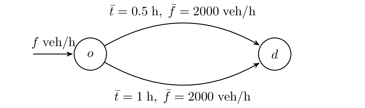
Refer to caption
Figure 1: Parallel routes

Let the input flow take values 1000, 2000, and 3000 veh/h. For the stable dynamics model, in the first and second cases, all drivers choose the upper route; the equilibrium travel time simply equals the upper route’s free flow time (0.5 h) in the first case and varies from 0.5 h to 1 h (according to the model) in the second. In the third case, the input flow exceeds the upper route’s capacity, so the upper route’s flow is 2000 veh/h, the lower one’s is 1000 veh/h, and the equilibrium travel time is 1 h. All these equilibria can be interpreted as stationary regimes of some dynamic processes, e.g. the last case can be viewed as the result of the queue at the beginning of the upper route (since this route’s capacity is smaller than the input flow) created by drivers who wanted to take this route until the waiting time plus the route’s travel time reached the lower route’s travel time (Nesterov and De Palma 2003). In the Beckmann model equilibria are as follows: for all three cases only the upper route is used, and the equilibrium travel times are approximately 0.5 h, 0.6 h, and 0.9 h, respectively. Chudak et al. 2007 conducted a detailed comparison — for large and small networks — of equilibria in these two models.

In the Beckmann model, searching equilibria reduces to minimization of a potential function. One of the most popular and effective approaches to solve this problem numerically is the famous Frank–Wolfe method (Frank and Wolfe 1956; Jaggi 2013) as well as its numerous modifications (Fukushima 1984; LeBlanc et al. 1985; Arezki and Van Vliet 1990; Chen et al. 2002).

In the case of the stable dynamics model, one cannot directly apply the Frank–Wolfe method. However, an equilibrium can be found as a solution of a pair of primal and dual optimization problems. The same holds also for the Beckmann model, so in both cases we can apply primal-dual (sub)gradient methods.

In this work, we compare several primal-dual gradient methods for searching equilibria in both the Beckmann and the stable dynamics models, namely, the universal gradient method (UGM) (Nesterov 2015), the universal method of similar triangles (UMST) (Gasnikov and Nesterov 2018), and the method of weighted dual averages (WDA) (Nesterov 2009). The main advantage of the above universal methods is an automatic adjustment to a local (Hölder) smoothness of a minimized function, which is especially important since the dual problems we are dealing with are essentially non-smooth. Due to the primal-dual nature of these methods, one can use an adaptive stopping criterion guaranteeing required accuracy.

The main contributions of this paper include the following:

  • •

    We propose a novel way to reconstruct admissible flows (i.e., meeting the capacity constraints and induced by flows on the paths) in the stable dynamics model and a novel computable duality gap, which can be used in a stopping criterion.

  • •

    We provide theoretical upper bounds on the complexity of searching equilibria by the considered algorithms: UMST, UGD, and WDA.

  • •

    We conducted numerical experiments comparing these algorithms on the Anaheim transportation network—the source code is available for use and can be found in Kubentayeva 2021.

The paper is organized as follows. In Section 2 we give a problem statement, define equilibria in the Beckmann and the stable dynamics models and corresponding optimization problems. Section 3 is devoted to the complexity analysis of UGM, UMST, and WDA. We show that the number of iterations required to obtain an ε\varepsilon-solution of primal and dual problems is O⁡(1/ε2)O(1/\varepsilon^{2}) for UGM and UMST. In Section 4 results of experiments on Anaheim transportation network are presented. Finally, some conclusions are drawn in Section 5.

2 Problem statement

Let the urban road network be represented by a directed graph G=(V,E)G=(V,E), where vertices VV correspond to intersections or centroids (Sheffi 1985) and edges EE correspond to roads, respectively. Suppose we are given the travel demands: namely, let dwd_{w}(veh/h) be a trip rate for an origin-destination pair ww from the set OD⊆{w=(i,j):i∈O,j∈D}OD\subseteq\{w=(i,j):i\in O,\;j\in D\}. Here O⊆VO\subseteq V is the set of all possible origins of trips, and D⊆VD\subseteq V is the set of destination nodes. For OD pair w=(i,j)w=(i,j) denote by PwP_{w} the set of all simple paths from ii to jj. Respectively, P=⋃w∈O​DPwP=\bigcup_{w\in OD}P_{w} is the set of all possible routes for all OD pairs. Agents traveling from node ii to node jj are distributed among paths from PwP_{w}, i.e. for any p∈Pwp\in P_{w} there is a flow xp∈ℝ+x_{p}\in\mathbb{R}_{+} along the path pp, and ∑p∈Pwxp=dw\sum_{p\in P_{w}}x_{p}=d_{w}. Flows from vertices from the set OO to vertices from the set DD create the traffic in the entire network GG, which can be represented by an element of

X={x∈ℝ+|P|:∑p∈Pwxp=dw,w∈OD}.X=\Bigl\{x\in\mathbb{R}_{+}^{|P|}:\;\sum_{p\in P_{w}}x_{p}=d_{w},\;w\in OD\Bigr\}.

Note that the dimension of XX can be extremely large: e.g. for n×nn\times n Manhattan network log⁡|P|=Ω⁡(n)\log|P|=\Omega(n). To describe a state of the network we do not need to know an entire vector xx, but only flows on arcs:

fe​(x)=∑p∈Pδe​p​xpfore∈E,f_{e}(x)=\sum_{p\in P}\delta_{ep}x_{p}\quad\text{for}\quad e\in E,

where δe​p=𝟙{e∈p}\delta_{ep}=\mathbbm{1}\{e\in p\}. Let us introduce a matrix Θ\Theta such that Θe,p=δe​p\Theta_{e,p}=\delta_{ep} for e∈Ee\in E, p∈Pp\in P, so in vector notation we have f=Θ​xf=\Theta x. To describe an equilibrium we use both path- and link-based notations (x,t)(x,t) or (f,t)(f,t).

Beckmann model. One of the key ideas behind the Beckmann model is that the cost (e.g. travel time, gas expenses, etc.) of passing a link ee is the same for all agents and depends solely on the flow fef_{e} along it. In what follows, we denote this cost for a given flow fef_{e} by te=τe​(fe)t_{e}=\tau_{e}(f_{e}). Another essential point is a behavioral assumption on agents called the first Wardrop’s principle: we suppose that each of them knows the state of the whole network and chooses a path pp minimizing the total cost

Tp​(t)=∑e∈pte.T_{p}(t)=\sum_{e\in p}t_{e}.

The cost functions are supposed to be continuous, non-decreasing, and non-negative. Then (x∗,t∗)(x^{*},t^{*}), where t∗=(te∗)e∈Et^{*}=(t_{e}^{*})_{e\in E}, is an equilibrium state, i.e. it satisfies conditions

te∗=τe​(fe∗),wheref∗=Θ​x∗,\displaystyle t_{e}^{*}=\tau_{e}(f_{e}^{*}),\quad\text{where}\quad f^{*}=\Theta x^{*},
xpw∗>0⟹Tpw​(t∗)=Tw​(t∗)=minp∈Pw⁡Tp​(t∗),\displaystyle x^{*}_{p_{w}}>0\Longrightarrow T_{p_{w}}(t^{*})=T_{w}(t^{*})=\min_{p\in P_{w}}T_{p}(t^{*}),

if and only if x∗x^{*} is a minimum of the potential function:

Ψ⁡(x)=∑e∈E∫0feτe​(z)​dz⏟σe​(fe)⟶minf=Θ​x,x∈X\displaystyle\Psi(x)=\sum_{e\in E}\underbrace{\int_{0}^{f_{e}}\tau_{e}(z)dz}_{\sigma_{e}(f_{e})}\longrightarrow\min_{f=\Theta x,\;x\in X}
⟺Ψ(f)=∑e∈Eσe(fe)⟶minf=Θ​x:x∈X,\displaystyle\Longleftrightarrow\Psi(f)=\sum_{e\in E}\sigma_{e}(f_{e})\longrightarrow\min_{f=\Theta x:\;x\in X}, (B)

and te∗=τe​(fe∗)t_{e}^{*}=\tau_{e}(f_{e}^{*}) (Beckmann et al. 1956).

Another way to find an equilibrium numerically is by solving a dual problem. According to Theorem 4 from Nesterov and De Palma 2003, we can construct it in the following way:

minf=Θ​x:x∈XΨ(f)\displaystyle\min_{f=\Theta x:\;x\in X}\Psi(f) =minx∈X,f⁡[Ψ⁡(f)+supt∈ℝ|E|⟨t,Θ​x−f⟩]=supt∈ℝ|E|minx∈X,f⁡[Ψ⁡(f)+⟨t,Θ​x−f⟩]\displaystyle=\min_{x\in X,\;f}\left[\Psi(f)+\sup_{t\in\mathbb{R}^{|E|}}\langle t,\Theta x-f\rangle\right]=\sup_{t\in\mathbb{R}^{|E|}}\min_{x\in X,\;f}\left[\Psi(f)+\langle t,\Theta x-f\rangle\right]
=supt∈ℝ|E|[−∑e∈Emaxfe{tefe−σe(fe)}+minx∈X∑p∑e∈Eteδe​pxp]\displaystyle=\sup_{t\in\mathbb{R}^{|E|}}\left[-\sum_{e\in E}\max_{f_{e}}\{t_{e}f_{e}-\sigma_{e}(f_{e})\}+\min_{x\in X}\sum_{p}\sum_{e\in E}t_{e}\delta_{ep}x_{p}\right]
=maxt∈dom⁡σ∗−[∑e∈Eσe∗​(te)−∑w∈O​Ddw​Tw​(t)]=−mint≥t¯⁡Q⁡(t),\displaystyle=\max_{t\in\dom\sigma^{*}}-\left[\sum_{e\in E}\sigma_{e}^{*}(t_{e})-\sum_{w\in OD}d_{w}T_{w}(t)\right]=-\min_{t\geq\bar{t}}Q(t),

where

σe∗​(te)=supfe≥0{te​fe−σe​(fe)}=f¯e​(te−t¯et¯e​ρ)μ​(te−t¯e)1+μ\sigma_{e}^{*}(t_{e})=\sup_{f_{e}\geq 0}\{t_{e}f_{e}-\sigma_{e}(f_{e})\}=\bar{f}_{e}\left(\frac{t_{e}-\bar{t}_{e}}{\bar{t}_{e}\rho}\right)^{\mu}\frac{\left(t_{e}-\bar{t}_{e}\right)}{1+\mu}

is the conjugate function of σe​(fe)\sigma_{e}(f_{e}), e∈Ee\in E. Finally, we obtain the dual problem, the solution of which is t∗t^{*}:

Q(t)=−∑w∈O​DdwTw(t)+∑e∈Eσe∗(te)⟶mint≥t¯.Q(t)=-\sum_{w\in OD}d_{w}T_{w}(t)+\sum_{e\in E}\sigma_{e}^{*}(t_{e})\longrightarrow\min_{t\geq\bar{t}}. (DualB)

When we search for the solution to this problem numerically, on every step of an applied method we can reconstruct primal variable ff from the current dual variable tt: f∈∂∑w∈O​Ddw​Tw​(t)f\in\partial\sum_{w\in OD}d_{w}T_{w}(t) (see Subsection 3.1). Then we can use the duality gap — which is always nonnegative — for the estimation of the method’s accuracy:

Δ⁡(f,t)=Ψ⁡(f)+Q⁡(t).\Delta(f,t)=\Psi(f)+Q(t).

It vanishes only at the equilibrium (f∗,t∗)(f^{*},t^{*}).

Stable dynamics model (Nesterov and De Palma 2003). An equilibrium state (x∗,t∗)(x^{*},t^{*}) of the stable dynamics model satisfies the next conditions:

te∗∈τe​(fe∗),\displaystyle t_{e}^{*}\in\tau_{e}(f_{e}^{*}),
xpw∗>0⟹Tpw​(t∗)=Tw​(t∗),\displaystyle x^{*}_{p_{w}}>0\Longrightarrow T_{p_{w}}(t^{*})=T_{w}(t^{*}),

where τ⁡(f)\tau(f) is defined earlier by (2). The above formula can be reformulated in terms of an optimization problem:

x∗\displaystyle x^{*} =arg​minx∈X∑w∈OD∑p∈PwxpTp(t∗)\displaystyle=\argmin\limits_{x\in X}\sum_{w\in OD}\sum_{p\in P_{w}}x_{p}T_{p}(t^{*})
=arg​minx∈X∑e∈Ete∗fe(x)\displaystyle=\argmin\limits_{x\in X}\sum_{e\in E}t^{*}_{e}f_{e}(x)
=arg​minx∈X∑e∈E[te∗fe(x)−(te∗−t¯e)​f¯e¯],\displaystyle=\argmin_{x\in X}\sum_{e\in E}[t^{*}_{e}f_{e}(x)-\underline{(t_{e}^{*}-\bar{t}_{e})\bar{f}_{e}}],
te∗∈τe​(fe∗)⟺te∗\displaystyle t_{e}^{*}\in\tau_{e}(f_{e}^{*})\Longleftrightarrow t_{e}^{*} =arg​maxte≥t¯e⁡te​(fe∗−f¯e)\displaystyle=\argmax_{t_{e}\geq\bar{t}_{e}}t_{e}(f_{e}^{*}-\bar{f}_{e})
=arg​maxte≥t¯e⁡[te​(fe∗−f¯e)+t¯e​f¯e¯].\displaystyle=\argmax_{t_{e}\geq\bar{t}_{e}}[t_{e}(f_{e}^{*}-\bar{f}_{e})+\underline{\bar{t}_{e}\bar{f}_{e}}].

Here, we add underlined constant terms to show that the pair (f∗,t∗)(f^{*},t^{*}) is an equilibrium if and only if it is a solution of the saddle-point problem

∑e∈E[tefe−(te−t¯e)f¯e]⟶minf=Θ​x:x∈Xmaxte≥t¯e,\sum_{e\in E}[t_{e}f_{e}-(t_{e}-\bar{t}_{e})\bar{f}_{e}]\longrightarrow\min_{\begin{subarray}{c}f=\Theta x:\\ x\in X\end{subarray}}\max_{t_{e}\geq\bar{t}_{e}}, (SaddleSD)

where its primal problem is

Ψ(x)=supte≥t¯e∑e∈E[tefe−(te−t¯e)f¯e]=∑e∈Et¯efe+∑e∈Esupte≥t¯e(te−t¯e)(fe−f¯e)⟶minf=Θ​x:x∈X\displaystyle\Psi(x)=\sup_{t_{e}\geq\bar{t}_{e}}\sum_{e\in E}[t_{e}f_{e}-(t_{e}-\bar{t}_{e})\bar{f}_{e}]=\sum_{e\in E}\bar{t}_{e}f_{e}+\sum_{e\in E}\sup_{t_{e}\geq\bar{t}_{e}}(t_{e}-\bar{t}_{e})(f_{e}-\bar{f}_{e})\longrightarrow\min_{f=\Theta x:x\in X}
⟺Ψ(f)=∑e∈Efet¯e⟶minf=Θ​x:x∈X,fe≤f¯e,\displaystyle\Longleftrightarrow\Psi(f)=\sum_{e\in E}f_{e}\bar{t}_{e}\longrightarrow\min_{\begin{subarray}{c}f=\Theta x:\\ x\in X,\,f_{e}\leq\bar{f}_{e}\end{subarray}}, (SD)

and its dual problem is

Q⁡(t)\displaystyle Q(t) =−inff=Θ​x:x∈X∑e∈E[tefe−(te−t¯e)f¯e]\displaystyle=-\inf_{f=\Theta x:x\in X}\sum_{e\in E}[t_{e}f_{e}-(t_{e}-\bar{t}_{e})\bar{f}_{e}]
=−∑w∈O​DdwTw(t)+⟨t−t¯,f¯⟩⟶minte≥t¯e.\displaystyle=-\sum_{w\in OD}d_{w}T_{w}(t)+\langle t-\bar{t},\bar{f}\rangle\longrightarrow\min_{t_{e}\geq\bar{t}_{e}}. (DualSD)

In contrast with the Beckmann model, the equilibrium state in the stable dynamics model is defined by pair (f∗,t∗)(f^{*},t^{*}) (in particular, it differs from the system optimum (f∗,t¯)(f^{*},\bar{t}) in the model only by the time value).

3 Numerical methods

We have the following objective functions

  • •

    The stable dynamics model:

    Q⁡(t)=−∑w∈O​DdwTw(t)⏟Φ⁡(t)+⟨t−t¯,f¯⟩⏟h⁡(t),Q(t)=\underbrace{-\sum_{w\in OD}d_{w}T_{w}(t)}_{\Phi(t)}+\underbrace{\langle t-\bar{t},\bar{f}\rangle}_{h(t)},
  • •

    The Beckmann model:

    Q⁡(t)=−∑w∈O​DdwTw(t)⏟Φ⁡(t)+∑e∈Ef¯e​(te−t¯et¯e​ρ)μ​(te−t¯e)1+μ⏟h⁡(t).Q(t)=\underbrace{-\sum_{w\in OD}d_{w}T_{w}(t)}_{\Phi(t)}+\underbrace{\sum_{e\in E}\bar{f}_{e}\left(\frac{t_{e}-\bar{t}_{e}}{\bar{t}_{e}\rho}\right)^{\mu}\frac{\left(t_{e}-\bar{t}_{e}\right)}{1+\mu}}_{h(t)}.

In both cases it has form

Q⁡(t)=Φ⁡(t)+h⁡(t)⟶mint≥t¯.Q(t)=\Phi(t)+h(t)\longrightarrow\min_{t\geq\bar{t}}. (3)

The optimization problem (3) is convex, non-smooth and composite. We use all these properties to identify the best optimization method to solve the considered problem.

3.1 Subgradient

In our research, we consider first-order methods, i.e. they require a subgradient of Φ⁡(t)\Phi(t), the properties and effective computation of which we discuss in this section.

To get the subdifferential ∂⁡Φ⁡(t)\sgr\Phi(t) let us re-write Φ⁡(t)\Phi(t) in the following way:

Φ(t)=−∑w∈O​DdwTw(t)=−∑w∈O​Ddwminp∈Pw⟨t,ap⟩,\Phi(t)=-\sum_{w\in OD}d_{w}T_{w}(t)=-\sum_{w\in OD}d_{w}\min_{p\in P_{w}}\langle t,a_{p}\rangle,

where the vector ap=(δe​p)e∈Ea_{p}=(\delta_{ep})_{e\in E} encodes a path pp. Obviously, the shortest path may not be unique. Using the rules of subgradient calculus (Rockafellar 2015) we get the following expression:

∂Φ(t)=−∑w∈ODdw∂(minp∈Pw⟨t,ap⟩)=−∑w∈ODdwConv{ap:p∈Pw,Tp(t)=Tw(t)},\sgr\Phi(t)=-\sum_{w\in OD}d_{w}\sgr\left(\min_{p\in P_{w}}\langle t,a_{p}\rangle\right)=-\sum_{w\in OD}d_{w}\mathrm{Conv}\{a_{p}:p\in P_{w},\;T_{p}(t)=T_{w}(t)\},

i.e. the subdifferential ∂⁡Φ⁡(t)\sgr\Phi(t) is a sum of convex hulls of binary vectors that encode the shortest length paths. An important consequence is that for any t1,t2∈ℝ+|E|t_{1},t_{2}\in\mathbb{R}_{+}^{|E|} and ∇Φ​(t1)∈∂⁡Φ⁡(t1)\nabla\Phi(t_{1})\in\sgr\Phi(t_{1}), ∇Φ​(t2)∈∂⁡Φ⁡(t2)\nabla\Phi(t_{2})\in\sgr\Phi(t_{2}) the following bound holds:

‖∇Φ​(t1)−∇Φ​(t2)‖2≤M=2​H​∑w∈O​Ddw,\left\lVert\nabla\Phi(t_{1})-\nabla\Phi(t_{2})\right\rVert_{2}\leq M=\sqrt{2H}\sum_{w\in OD}d_{w}, (4)

where HH is the diameter of the graph GG.

Note that any element from the set ∂⁡Φ⁡(t)\sgr\Phi(t) has form ∇Φ​(t)=−f\nabla\Phi(t)=-f, where f=Θ​xf=\Theta x is a flow distribution on links induced by x∈Xx\in X concentrated on the shortest paths for given times tt (and vice versa: any such ff corresponds to a subgradient of Φ⁡(t)\Phi(t)).

In practice, the calculation of flows ff is the most expensive part, since we have to find the shortest paths for all pairs w∈O​Dw\in OD. We use the following algorithm 1. We use Dijkstra’s algorithm (Dijkstra et al. 1959) to find the shortest paths in line 3, which runs in O⁡(|E|+|V|​log⁡|V|)O(|E|+|V|\log|V|) time; finding the traversal order with topological sort (Section 22.4 in Cormen et al. 2009) and further flows aggregation have linear performance O⁡(|V|)O(|V|). Hence, the total complexity of Algorithm 1 is O⁡(|O|​(|E|+|V|​log⁡|V|))O\bigl(|O|(|E|+|V|\log|V|)\bigr). When the transportation network is an (almost) planar graph or another sparse graph, |E|=O⁡(|V|)|E|=O(|V|) and the complexity is O⁡(|O|⋅|V|​log⁡|V|)O(|O|\cdot|V|\log|V|). Moreover, flows reconstruction for every source o∈Oo\in O can be computed in parallel. And Dijkstra’s algorithm also can be parallelized and has efficient implementations (Crauser et al. 1998; Chao and Hongxia 2010).

Algorithm 1 Flows reconstruction
0:  times tt
1:  f≔𝟎|E|f\coloneqq\bm{0}_{|E|} {flows on edges}
2:  for origin oo in OO do
3:   Get a shortest-path tree 𝒯o\mathcal{T}_{o} from oo to all destinations in DD with weights tt
4:   traversal​_​order≔TopologicalSort⁡(𝒯o)\mathrm{traversal\_order}\coloneqq\mathrm{TopologicalSort}(\mathcal{T}_{o}) {sorting from furthest to closest vertices}
5:   fout≔𝟎|V|f_{\mathrm{out}}\coloneqq\bm{0}_{|V|} {total output flow from each vertex}
6:   fout​[v]≔dwf_{\mathrm{out}}[v]\coloneqq d_{w} for w=(o,v)∈O​Dw=(o,v)\in OD
7:   for vv in traversal​_​order\mathrm{traversal\_order} do
8:    Get predecessor pp of vv in 𝒯o\mathcal{T}_{o}
9:    e≔(p,v)e\coloneqq(p,v)
10:    f⁡[e]≔f⁡[e]+fout​[v]f[e]\coloneqq f[e]+f_{\mathrm{out}}[v]
11:    fout​[p]≔fout​[p]+fout​[v]f_{\mathrm{out}}[p]\coloneqq f_{\mathrm{out}}[p]+f_{\mathrm{out}}[v]
12:   end for
13:  end for
14:  return flows ff

3.2 Reconstruction of admissible flows in SD model

For given times tt considered Algorithm 1 reconstructs feasible flows ff, i.e. f=Θ​xf=\Theta x for some x∈Xx\in X. These flows meet all the constraints in the Beckmann model, but they can violate the capacity constraints in the stable dynamics model. In the latter case, an additional step is required to obtain admissible flows from ff. Note that we could instead find flows that meet capacity constraints first (Theorem 8 from Nesterov and De Palma 2003), but to reconstruct feasible flows from them is a more complex problem.

Suppose we are given some flows g=Θ​xg=\Theta x such that

ξ=1−maxe∈E⁡ge/f¯e>0.\xi=1-\max_{e\in E}g_{e}/\bar{f}_{e}>0. (5)

Then for any f=Θ​xf=\Theta x we can construct admissible flows π⁡(f)\pi(f) in the following way: let η=maxe∈E⁡fe/f¯e−1\eta=\max_{e\in E}f_{e}/\bar{f}_{e}-1, then

π⁡(f)={f,η≤0,ξ​f+η​gξ+η,η>0.\pi(f)=\begin{cases}f,&\eta\leq 0,\\ \frac{\xi f+\eta g}{\xi+\eta},&\eta>0.\end{cases}

In practice, we propose the following procedure to find admissible flows gg: run some optimization method (e.g. UGM) for a small number of iterations for the same problem but with decreased capacities: 12​f¯\frac{1}{2}\bar{f} instead of f¯\bar{f}; if obtained feasible flows f^N\hat{f}^{N} satisfy f^N≤34​f¯\hat{f}^{N}\leq\frac{3}{4}\bar{f}, then take g=f^Ng=\hat{f}^{N}; otherwise, run it again with capacities 34​f¯\frac{3}{4}\bar{f} and check f^N≤78​f¯\hat{f}^{N}\leq\frac{7}{8}\bar{f}, etc.

Stopping criterion.

The stopping criterion we use for the stable dynamics model is based on a duality gap

Q⁡(t^N)+Ψ⁡(π⁡(f^N))≤ε,Q(\hat{t}^{N})+\Psi(\pi(\hat{f}^{N}))\leq\varepsilon, (6)

where f^N∈{Θ​x:x∈X}\hat{f}^{N}\in\left\{\Theta x:x\in X\right\}, t^N≥t¯\hat{t}^{N}\geq\bar{t} are estimates of an equilibrium (f∗,t∗)(f^{*},t^{*}) after NN iterations of the applied method. Note that here the duality gap with f^N\hat{f}^{N} is not applicable.

3.3 Universal gradient method

The method for solving non-smooth problems with smooth techniques was proposed by Nesterov 2015 and was called the universal gradient method. The pseudocode of UGM for the considered problem (3) is provided in Algorithm 2. Here the euclidean prox-structure is used. Note that we did not specify the stopping criterion as it can be different for different models.

Algorithm 2 Universal gradient method
0:  L0>0L_{0}>0, accuracy ε>0\varepsilon>0
1:  Set t0≔t¯t^{0}\coloneqq\bar{t}, k≔0k\coloneqq 0
2:  repeat
3:   Lk+1≔Lk/2L_{k+1}\coloneqq L_{k}/2
4:   while true do
5:    tk+1≔arg​mint∈dom⁡h⁡⟨∇Φ​(tk),t−tk⟩+h⁡(t)+Lk+1​‖t−tk‖222t^{k+1}\coloneqq\argmin\limits_{t\in\dom h}\langle\nabla\Phi(t^{k}),t-t^{k}\rangle+h(t)+L_{k+1}\frac{\left\lVert t-t^{k}\right\rVert_{2}^{2}}{2}
6:    if Φ⁡(tk+1)≤Φ⁡(tk)+⟨∇Φ​(tk),tk+1−tk⟩+Lk+1​‖tk+1−tk‖222+ε2\Phi(t^{k+1})\leq\Phi(t^{k})+\left\langle\nabla\Phi(t^{k}),t^{k+1}-t^{k}\right\rangle+L_{k+1}\frac{\left\lVert t^{k+1}-t^{k}\right\rVert_{2}^{2}}{2}+\frac{\varepsilon}{2} then
7:     break
8:    else
9:     Lk+1≔2​Lk+1L_{k+1}\coloneqq 2L_{k+1}
10:    end if
11:   end while
12:   k≔k+1k\coloneqq k+1
13:  until Stopping criterion is fulfilled

Now let us define

f^N=−1SN∑k=0N−1∇Φ​(tk)Lk+1,t^N=1SN∑k=1NtkLk,SN=∑k=1N1Lk,\hat{f}^{N}=-\frac{1}{S_{N}}\sum_{k=0}^{N-1}\frac{\nabla\Phi(t^{k})}{L_{k+1}},\quad\hat{t}^{N}=\frac{1}{S_{N}}\sum_{k=1}^{N}\frac{t^{k}}{L_{k}},\quad S_{N}=\sum_{k=1}^{N}\frac{1}{L_{k}}, (7)

where LkL_{k} are the estimates of the local Lipschitz constant in UGM and UMST methods.

Convergence of the UGM was proved in Nesterov 2015 and is summarized in the following lemma and theorem.

Lemma 3.1.

After NN iterations of UGM for the stable dynamics model it holds that

Q⁡(t^N)−Q⁡(t∗)≤R2SN+ε2,\displaystyle Q(\hat{t}^{N})-Q(t^{*})\leq\frac{R^{2}}{S_{N}}+\frac{\varepsilon}{2}, (8)
0≤Q⁡(t^N)+Ψ⁡(f^N)+⟨t∗−t¯,(f^N−f¯)+⟩≤R2SN+ε2,\displaystyle 0\leq Q(\hat{t}^{N})+\Psi(\hat{f}^{N})+\langle t^{*}-\bar{t},(\hat{f}^{N}-\bar{f})_{+}\rangle\leq\frac{R^{2}}{S_{N}}+\frac{\varepsilon}{2}, (9)
∥(f^N−f¯)+∥2≤4​RSN+2​εSN,\displaystyle\lVert(\hat{f}^{N}-\bar{f})_{+}\rVert_{2}\leq\frac{4R}{S_{N}}+\sqrt{\frac{2\varepsilon}{S_{N}}}, (10)

where f^N\hat{f}^{N}, t^N\hat{t}^{N}, and SNS_{N} are defined by (7), and R=∥t∗−t¯∥2R=\lVert t^{*}-\bar{t}\rVert_{2} is the distance from the starting point to a solution.

Theorem 3.2.

Let L0≤M2εL_{0}\leq\frac{M^{2}}{\varepsilon}, where MM comes from (4). Then after at most

NQ=2​(R​Mε)2N_{Q}=2\left(\frac{RM}{\varepsilon}\right)^{2} (11)

iterations of UGM for the stable dynamics model it holds that Q⁡(t^N)−Q⁡(t∗)≤εQ(\hat{t}^{N})-Q(t^{*})\leq\varepsilon. Moreover, the stopping criterion (6) is fulfilled after at most

Ns​t​o​p=O⁡((R​Mε)2​max⁡{1,(⟨g−f∗,t¯⟩ξ​R​mine​f¯e)2})N_{stop}=O\left(\left(\frac{RM}{\varepsilon}\right)^{2}\max\left\{1,\,\left(\frac{\langle g-f^{*},\bar{t}\rangle}{\xi R\min_{e}\bar{f}_{e}}\right)^{2}\right\}\right) (12)

iterations, where ξ\xi comes from (5).

Now we provide results on the rate of convergence for the Beckmann model. The stopping criterion in this case is the following:

Q⁡(t^N)+Ψ⁡(f^N)≤ε.Q(\hat{t}^{N})+\Psi(\hat{f}^{N})\leq\varepsilon. (13)
Lemma 3.3.

After NN iterations of UGM for the Beckmann model it holds that

Q⁡(t^N)−Q⁡(t∗)≤R2SN+ε2,\displaystyle Q(\hat{t}^{N})-Q(t^{*})\leq\frac{R^{2}}{S_{N}}+\frac{\varepsilon}{2},
0≤Q⁡(t^N)+Ψ⁡(f^N)≤∥τ⁡(f^N)−t¯∥22SN+ε2,\displaystyle 0\leq Q(\hat{t}^{N})+\Psi(\hat{f}^{N})\leq\frac{\lVert\tau(\hat{f}^{N})-\bar{t}\rVert_{2}^{2}}{S_{N}}+\frac{\varepsilon}{2},

where f^N\hat{f}^{N}, t^N\hat{t}^{N}, SNS_{N} are defined by (7), and R=∥t∗−t¯∥2R=\lVert t^{*}-\bar{t}\rVert_{2}

Theorem 3.4.

Let L0≤M2εL_{0}\leq\frac{M^{2}}{\varepsilon}, where MM comes from (4). Then after at most

NQ=2​(R​Mε)2N_{Q}=2\left(\frac{RM}{\varepsilon}\right)^{2} (14)

iterations of UGM for the Beckmann model it holds that Q⁡(t^N)−Q⁡(t∗)≤εQ(\hat{t}^{N})-Q(t^{*})\leq\varepsilon. Moreover, the stopping criterion (13) is fulfilled after at most

Ns​t​o​p=2​(R~​Mε)2N_{stop}=2\left(\frac{\tilde{R}M}{\varepsilon}\right)^{2} (15)

iterations, where

R~2=ρ2​∑e∈Et¯e2f¯e2/μ​(∑w∈O​Ddw)2/μ.\tilde{R}^{2}=\rho^{2}\sum_{e\in E}\frac{\bar{t}_{e}^{2}}{\bar{f}_{e}^{2/\mu}}\left(\sum_{w\in OD}d_{w}\right)^{2/\mu}. (16)

3.4 Universal Method of Similar Triangles

Let us introduce the following notations:

ϕ0​(t)=12​‖t−t0‖22,\phi_{0}(t)=\frac{1}{2}\left\lVert t-t^{0}\right\rVert_{2}^{2},
ϕk+1​(t)=ϕk​(t)+αk+1​[Φ⁡(yk+1)+⟨∇Φ​(yk+1),t−yk+1⟩+h⁡(t)].\phi_{k+1}(t)=\phi_{k}(t)+\alpha_{k+1}\left[\Phi(y^{k+1})+\left\langle\nabla\Phi(y^{k+1}),t-y^{k+1}\right\rangle+h(t)\right].
Algorithm 3 Universal Method of Similar Triangles
0:  L0>0L_{0}>0, accuracy ε>0\varepsilon>0
1:  u0=t0≔t¯u^{0}=t^{0}\coloneqq\bar{t}, A0≔0A_{0}\coloneqq 0, k≔0k\coloneqq 0
2:  repeat
3:   Lk+1≔Lk/2L_{k+1}\coloneqq L_{k}/2
4:   while true do
5:    {αk+1≔12​Lk+1+14​Lk+12+AkLk+1,Ak+1≔Ak+αk+1yk+1≔αk+1​uk+Ak​tkAk+1,uk+1≔arg​mint∈dom⁡h⁡ϕk+1​(t)tk+1≔αk+1​uk+1+Ak​tkAk+1\begin{cases}\alpha_{k+1}\coloneqq\frac{1}{2L_{k+1}}+\sqrt{\frac{1}{4L_{k+1}^{2}}+\frac{A_{k}}{L_{k+1}}},\quad A_{k+1}\coloneqq A_{k}+\alpha_{k+1}\\ y^{k+1}\coloneqq\frac{\alpha_{k+1}u^{k}+A_{k}t^{k}}{A_{k+1}},\quad u^{k+1}\coloneqq\argmin\limits_{t\in\dom h}\phi_{k+1}(t)\\ t^{k+1}\coloneqq\frac{\alpha_{k+1}u^{k+1}+A_{k}t^{k}}{A_{k+1}}\end{cases}
6:    if Φ⁡(tk+1)≤Φ⁡(yk+1)+⟨∇Φ​(yk+1),tk+1−yk+1⟩+Lk+12​‖tk+1−yk+1‖22+αk+12​Ak+1​ε\Phi(t^{k+1})\leq\Phi(y^{k+1})+\left\langle\nabla\Phi(y^{k+1}),t^{k+1}-y^{k+1}\right\rangle+\frac{L_{k+1}}{2}\left\lVert t^{k+1}-y^{k+1}\right\rVert_{2}^{2}+\frac{\alpha_{k+1}}{2A_{k+1}}\varepsilon then
7:     break
8:    else
9:     Lk+1≔2​Lk+1L_{k+1}\coloneqq 2L_{k+1}
10:    end if
11:   end while
12:   k≔k+1k\coloneqq k+1
13:  until Stopping criterion is fulfilled

Flows are reconstructed in the following way:

f^N=−1AN∑k=1Nαk∇Φ(yk)\hat{f}^{N}=-\frac{1}{A_{N}}\sum_{k=1}^{N}\alpha_{k}\nabla\Phi(y^{k}) (17)
Lemma 3.5.

After NN iterations of UMST for the stable dynamics model it holds that

Q⁡(tN)−Q⁡(t∗)≤R2AN+ε2,\displaystyle Q(t^{N})-Q(t^{*})\leq\frac{R^{2}}{A_{N}}+\frac{\varepsilon}{2}, (18)
0≤Q⁡(tN)+Ψ⁡(f^N)+⟨t∗−t¯,(f^N−f¯)+⟩≤R2AN+ε2,\displaystyle 0\leq Q(t^{N})+\Psi(\hat{f}^{N})+\langle t^{*}-\bar{t},(\hat{f}^{N}-\bar{f})_{+}\rangle\leq\frac{R^{2}}{A_{N}}+\frac{\varepsilon}{2}, (19)
∥(f^N−f¯)+∥2≤4​RAN+2​εAN,\displaystyle\lVert(\hat{f}^{N}-\bar{f})_{+}\rVert_{2}\leq\frac{4R}{A_{N}}+\sqrt{\frac{2\varepsilon}{A_{N}}}, (20)

where f^N\hat{f}^{N} is defined by (17) and R=∥t∗−t¯∥2R=\lVert t^{*}-\bar{t}\rVert_{2} is the distance from the starting point to a solution.

Theorem 3.6.

Let L0≤4​M2εL_{0}\leq\frac{4M^{2}}{\varepsilon}, where MM comes from (4). Then after at most

NQ=4​(R​Mε)2N_{Q}=4\left(\frac{RM}{\varepsilon}\right)^{2} (21)

iterations of UGM for the stable dynamics model it holds that Q⁡(tN)−Q⁡(t∗)≤εQ(t^{N})-Q(t^{*})\leq\varepsilon. Moreover, the stopping criterion (6) with t^N=tN\hat{t}^{N}=t^{N} is fulfilled after at most

Ns​t​o​p=O⁡((R​Mε)2​max⁡{1,(⟨g−f∗,t¯⟩ξ​R​mine​f¯e)2})N_{stop}=O\left(\left(\frac{RM}{\varepsilon}\right)^{2}\max\left\{1,\,\left(\frac{\langle g-f^{*},\bar{t}\rangle}{\xi R\min_{e}\bar{f}_{e}}\right)^{2}\right\}\right) (22)

iterations, where ξ\xi comes from (5).

Theorem 3.7.

Let L0≤4​M2εL_{0}\leq\frac{4M^{2}}{\varepsilon}, where MM comes from (4). Then after at most

NQ=4​(R​Mε)2N_{Q}=4\left(\frac{RM}{\varepsilon}\right)^{2} (23)

iterations of UMST for the Beckmann model it holds that Q⁡(tN)−Q⁡(t∗)≤εQ(t^{N})-Q(t^{*})\leq\varepsilon. Moreover, the stopping criterion (13) with t^N=tN\hat{t}^{N}=t^{N} is fulfilled after at most

Ns​t​o​p=4​(R~​Mε)2N_{stop}=4\left(\frac{\tilde{R}M}{\varepsilon}\right)^{2} (24)

iterations, where R~\tilde{R} is defined by (16).

3.5 Method of Weighted Dual Averages

Algorithm 4 Method of Weighted Dual Averages
0:  accuracy ε>0\varepsilon>0, constant χ>0\chi>0
1:  s0≔0→s^{0}\coloneqq\vec{0}, t0≔t¯t^{0}\coloneqq\bar{t}, k≔0k\coloneqq 0
2:  repeat
3:   Compute subgradient gkg^{k}, set sk+1≔sk+1∥gk∥2​gks^{k+1}\coloneqq s^{k}+\frac{1}{\lVert g^{k}\rVert_{2}}g^{k}
  • •

    non-composite case: gk≔∇Φ​(tk)+∇h​(tk)g^{k}\coloneqq\nabla\Phi(t^{k})+\nabla h(t^{k})

  • •

    composite case: gk≔∇Φ​(tk)g^{k}\coloneqq\nabla\Phi(t^{k})

4:   Set βk+1≔β^k+1χ\beta_{k+1}\coloneqq\frac{\hat{\beta}_{k+1}}{\chi}, where β^k+1=∑i=0k1β^i,β^0=1\hat{\beta}_{k+1}=\sum_{i=0}^{k}\frac{1}{\hat{\beta}_{i}},\;\hat{\beta}_{0}=1
5:   Set tk+1t^{k+1}
  • •

    non-composite case: tk+1≔arg​mint∈dom⁡h⁡⟨sk+1,t⟩+βk+12​‖t−t0‖22t^{k+1}\coloneqq\argmin\limits_{t\in\dom h}\langle s^{k+1},t\rangle+\frac{\beta_{k+1}}{2}\left\lVert t-t^{0}\right\rVert_{2}^{2}

  • •

    composite case: tk+1≔arg​mint∈dom⁡h⁡⟨sk+1,t⟩+βk+12​‖t−t0‖22+∑i=0k1∥gk∥2​h​(t)t^{k+1}\coloneqq\argmin\limits_{t\in\dom h}\langle s^{k+1},t\rangle+\frac{\beta_{k+1}}{2}\left\lVert t-t^{0}\right\rVert_{2}^{2}+\sum_{i=0}^{k}\frac{1}{\lVert g^{k}\rVert_{2}}h(t)

6:   k≔k+1k\coloneqq k+1
7:  until Stopping criterion is fulfilled

Convergence of WDA-method was proved in Nesterov 2009 and is summarized in the following theorem.

Theorem 3.8.

Non-composite WDA-method satisfies the following bounds

  • •

    for the stable dynamics model:

    Q⁡(t^k)−Q⁡(t∗)=O⁡(M+∥f¯∥2k​(R2χ+χ)),Q(\hat{t}^{k})-Q(t^{*})=O\left(\frac{M+\lVert\bar{f}\rVert_{2}}{\sqrt{k}}\left(\frac{R^{2}}{\chi}+\chi\right)\right),
  • •

    for the Beckmann model if μ≤1\mu\leq 1:

    Q⁡(t^k)−Q⁡(t∗)=O⁡(1k​(M+maxe⁡f¯e​[2​R+χt¯e​ρ]μ)​(R2χ+χ)).Q(\hat{t}^{k})-Q(t^{*})=O\left(\frac{1}{\sqrt{k}}\left(M+\max_{e}\bar{f}_{e}\left[\frac{2R+\chi}{\bar{t}_{e}\rho}\right]^{\mu}\right)\left(\frac{R^{2}}{\chi}+\chi\right)\right).

4 Numerical experiments

This section presents numerical results for the algorithms described above, namely, composite variants of UMST and UGM, both composite and non-composite WDA-method, on the Anaheim network (Transportation Networks for Research Core Team 2021; Chudak et al. 2007). The network consists of 38 zones, 416 nodes, and 916 links. Experiments and the source code in Python 3(Van Rossum and Drake 2009) can be found in Kubentayeva 2021. We used Dijkstra’s algorithm for finding the shortest paths in the network from the graph-tool library (Peixoto 2014), where it is implemented in C++. We also used the Numpy library (Harris et al. 2020) for all vector operations.

Stable dynamics model.

Parameters of the network are adjusted to the Beckmann model, so we have to increase the capacities to ensure the existence of an equilibrium for the stable dynamics model. In our experiments, the capacities are multiplied by 2.52.5. In Figure 2, we plot the number of (inner) iterations of the algorithms required to fulfill the stopping criterion (6) against 1/ε1/\varepsilon. We consider the number of inner iterations for Alg. 3 and Alg. 2 since the complexity of an inner iteration in this case is similar to the complexity of an iteration of the other algorithms. Note that according to (Nesterov 2015, formula (2.23)) the number N⁡(k)N(k) of inner iterations of UGM or UMST at step kk is bounded as

N⁡(k)≤2​k+log2⁡(M2ε​L0),N(k)\leq 2k+\log_{2}\left(\frac{M^{2}}{\varepsilon L_{0}}\right),

so asymptotic rates from Theorems 3.2, 3.4, 3.6, and 3.7 are still valid.

As we can see, the best results are shown by UMST, followed by UGM having similar performance. Both composite and non-composite WDA-method are much slower.

Refer to caption
Figure 2: Convergence rates of UMST, UGM, composite and non-composite WDA-methods for the stable dynamics model with the stopping criterion (6). Here ε~\tilde{\varepsilon} is the relative accuracy ε/Δ0\varepsilon/\Delta_{0}, where Δ0\Delta_{0} is the duality gap at the start point.

Beckmann model.

For the Beckmann model we also compare our methods with the Frank–Wolfe algorithm (Alg. 5) — which theoretical convergence rate for convex objective (with Lipschitz-continuous gradient) is O⁡(1/ε)O(1/\varepsilon) (Pedregosa et al. 2020; Jaggi 2013).

Algorithm 5 Frank-Wolfe algorithm
0:  accuracy ε>0\varepsilon>0
1:  t0≔t¯t^{0}\coloneqq\bar{t}, f0≔arg​mins∈{Θ​x:x∈X}⟨t0,s⟩f^{0}\coloneqq\argmin\limits_{s\in\{\Theta x:x\in X\}}\langle t^{0},s\rangle, k≔0k\coloneqq 0
2:  repeat
3:   sk≔arg​mins∈{Θ​x:x∈X}⟨tk,s⟩s^{k}\coloneqq\argmin\limits_{s\in\{\Theta x:x\in X\}}\langle t^{k},s\rangle, tek≔∂Ψ⁡(fk)∂fe=τe​(fk)t_{e}^{k}\coloneqq\frac{\partial\Psi(f^{k})}{\partial f_{e}}=\tau_{e}(f^{k})
4:   γk≔2k+2\gamma_{k}\coloneqq\frac{2}{k+2}, fk+1≔(1−γk)​fk+γk​skf^{k+1}\coloneqq(1-\gamma_{k})f^{k}+\gamma_{k}s^{k}
5:   k≔k+1k\coloneqq k+1
6:  until Stopping criterion is fulfilled

Figure 3 shows the convergence rates of the methods for the Beckmann model. The Frank–Wolfe method demonstrates the best results and is followed by UMST. Unlike the stable dynamics case, composite WDA-method is faster than UGM. However, the non-composite WDA-method has the worst performance again.

Refer to caption
Figure 3: Convergence rates of UMST, UGM, composite and non-composite WDA-methods, and the Frank–Wolfe method for the Beckmann model with the stopping criterion (13). Here ε~\tilde{\varepsilon} is the relative accuracy ε/Δ0\varepsilon/\Delta_{0}, where Δ0\Delta_{0} is the duality gap at the start point.

5 Conclusion

We considered several primal-dual subgradient methods for finding equilibria in the stable dynamics and the Beckmann models. We suggested a way to reconstruct admissible flows in the stable dynamics model, which provides us with a novel computable duality gap. Complexity bounds for UMST and UGM were presented in terms of the iterations number required to achieve a desired accuracy in the dual function value or the duality gap. Finally, we conducted numerical experiments comparing convergence of the considered algorithms on the Anaheim transportation network: UMST is the best one for optimization of the dual problems in both models. Also, using the duality gap as a stopping criterion, we compared these methods with the Frank–Wolfe algorithm for the Beckmann model — which, as expected, remains the most suitable approach in this case (but it is not applicable for the stable dynamics model).

The reader may be interested in another related topic, searching stochastic traffic equilibria. In Gasnikov and Kubentayeva 2018; Baimurzina et al. 2019 we with our colleagues studied the application of the UMST for finding Nash–Wardrop stochastic equilibria in the Beckmann model. In this case, a driver selects a route randomly according to Gibbs’ distribution taking into account current time costs on the links of the network. It leads to iteration complexity O⁡(1γ​ε)O(\frac{1}{\sqrt{\gamma\varepsilon}}), where γ>0\gamma>0 is a stochasticity parameter (when γ→0\gamma\to 0 the model boils down to the ordinary Beckmann model). However, the great decrease in the number of iterations comes along with a more expensive calculation of the objective function’s gradient.

Acknowledgements

We would like to thanks Yu. Nesterov for fruitful discussions.

The research of M. Kubentayeva was supported by Russian Science Foundation (project 18-71-10108).

The research of A. Gasnikov was partially supported by RFBR, project number 18-29-03071 mk, and was partially supported by the Ministry of Science and Higher Education of the Russian Federation (Goszadaniye) no 075-00337-20-03.

References

  • (1)
  • Arezki and Van Vliet (1990) Arezki, Y. and Van Vliet, D. (1990). A full analytical implementation of the PARTAN/Frank–Wolfe algorithm for equilibrium assignment, Transportation Science 24(1): 58–62.
  • Baimurzina et al. (2019) Baimurzina, D. R., Gasnikov, A. V., Gasnikova, E. V., Dvurechensky, P. E., Ershov, E. I., Kubentaeva, M. B. and Lagunovskaya, A. A. (2019). Universal method of searching for equilibria and stochastic equilibria in transportation networks, Computational Mathematics and Mathematical Physics 59(1): 19–33.
  • Beckmann et al. (1956) Beckmann, M. J., McGuire, C. B. and Winsten, C. B. (1956). Studies in the economics of transportation, Technical report.
  • Chao and Hongxia (2010) Chao, Y. and Hongxia, W. (2010). Developed Dijkstra shortest path search algorithm and simulation, 2010 International Conference on Computer Design and Applications, Vol. 1, IEEE, pp. V1–116.
  • Chen et al. (2002) Chen, A., Jayakrishnan, R. and Tsai, W. (2002). Faster Frank–Wolfe traffic assignment with new flow update scheme, Journal of Transportation Engineering-asce - J TRANSP ENG-ASCE 128.
  • Chudak et al. (2007) Chudak, F. A., Dos Santos Eleuterio, V. and Nesterov, Y. (2007). Static traffic assignment problem: A comparison between Beckmann (1956) and Nesterov & de Palma (1998) models, 7th Swiss Transport Research Conference, ETH.
  • Cormen et al. (2009) Cormen, T. H., Leiserson, C. E., Rivest, R. L. and Stein, C. (2009). Introduction to algorithms, 3rd-edition, MIT press.
  • Crauser et al. (1998) Crauser, A., Mehlhorn, K., Meyer, U. and Sanders, P. (1998). A parallelization of Dijkstra’s shortest path algorithm, International Symposium on Mathematical Foundations of Computer Science, Springer, pp. 722–731.
  • Dijkstra et al. (1959) Dijkstra, E. W. et al. (1959). A note on two problems in connexion with graphs, Numerische mathematik 1(1): 269–271.
  • Frank and Wolfe (1956) Frank, M. and Wolfe, P. (1956). An algorithm for quadratic programming, Naval research logistics quarterly 3(1-2): 95–110.
  • Fukushima (1984) Fukushima, M. (1984). A modified Frank–Wolfe algorithm for solving the traffic assignment problem, Transportation Research Part B: Methodological 18(2): 169–177.
  • Gasnikov and Kubentayeva (2018) Gasnikov, A. V. and Kubentayeva, M. B. (2018). Searching stochastic equilibria in transport networks by universal primal-dual gradient method, Computer research and modeling 10(3): 335–345.
  • Gasnikov and Nesterov (2018) Gasnikov, A. V. and Nesterov, Y. E. (2018). Universal method for stochastic composite optimization problems, Computational Mathematics and Mathematical Physics 58(1): 48–64.
  • Harris et al. (2020) Harris, C. R., Millman, K. J., van der Walt, S. J., Gommers, R., Virtanen, P., Cournapeau, D., Wieser, E., Taylor, J., Berg, S., Smith, N. J., Kern, R., Picus, M., Hoyer, S., van Kerkwijk, M. H., Brett, M., Haldane, A., del Río, J. F., Wiebe, M., Peterson, P., Gérard-Marchant, P., Sheppard, K., Reddy, T., Weckesser, W., Abbasi, H., Gohlke, C. and Oliphant, T. E. (2020). Array programming with NumPy, Nature 585(7825): 357–362.
    https://doi.org/10.1038/s41586-020-2649-2
  • Jaggi (2013) Jaggi, M. (2013). Revisiting Frank–Wolfe: Projection-free sparse convex optimization., Proceedings of the 30th international conference on machine learning, pp. 427–435.
  • Kubentayeva (2021) Kubentayeva, M. (2021). TransportNet, https://github.com/MeruzaKub/TransportNet. Accessed: 2021-04-30.
  • LeBlanc et al. (1985) LeBlanc, L. J., Helgason, R. V. and Boyce, D. E. (1985). Improved efficiency of the Frank–Wolfe algorithm for convex network programs, Transportation Science 19(4): 445–462.
  • Nesterov (2009) Nesterov, Y. (2009). Primal-dual subgradient methods for convex problems, Mathematical programming 120(1): 221–259.
  • Nesterov (2015) Nesterov, Y. (2015). Universal gradient methods for convex optimization problems, Mathematical Programming 152(1-2): 381–404.
  • Nesterov and De Palma (2003) Nesterov, Y. and De Palma, A. (2003). Stationary dynamic solutions in congested transportation networks: summary and perspectives, Networks and Spatial Economics 3(3): 371–395.
  • Patriksson (2015) Patriksson, M. (2015). The traffic assignment problem: models and methods, Courier Dover Publications.
  • Pedregosa et al. (2020) Pedregosa, F., Negiar, G., Askari, A. and Jaggi, M. (2020). Linearly convergent frank-wolfe with backtracking line-search, Proceedings of the 23rdInternational Conference on Artificial Intelligence and Statistics.
    https://arxiv.org/pdf/1806.05123.pdf
  • Peixoto (2014) Peixoto, T. P. (2014). The graph-tool python library, figshare .
    http://figshare.com/articles/graph_tool/1164194
  • Rockafellar (2015) Rockafellar, R. T. (2015). Convex analysis, Princeton university press.
  • Sheffi (1985) Sheffi, Y. (1985). Urban transportation networks, Vol. 6, Prentice-Hall, Englewood Cliffs, NJ.
  • Transportation Networks for Research Core Team (2021) Transportation Networks for Research Core Team (2021). Transportation networks for research, https://github.com/bstabler/TransportationNetworks. Accessed: 2021-04-30.
  • US Bureau of Public Roads (1964) US Bureau of Public Roads (1964). Traffic Assignment Manual, Department of Commerce, Urban Planning Division, Washington D.C.
  • Van Rossum and Drake (2009) Van Rossum, G. and Drake, F. L. (2009). Python 3 Reference Manual, CreateSpace, Scotts Valley, CA.

6 Appendix

6.1 Proofs for UGM

Proof of Lemma 3.1.

Note that function Φ⁡(t)\Phi(t) satisfies (4). Then according to Theorem 1 in Nesterov 2015 applied with ν=0\nu=0 one has

Q⁡(t^N)\displaystyle Q(\hat{t}^{N}) ≤1SN​∑k=1N1Lk​Q​(tk)\displaystyle\leq\frac{1}{S_{N}}\sum_{k=1}^{N}\frac{1}{L_{k}}Q(t^{k})
≤mint≥t¯⁡{1SN​∑k=0N−11Lk+1​[Φ⁡(tk)+⟨∇Φ​(tk),t−tk⟩]+h⁡(t)+∥t−t0∥22SN}+ε2.\displaystyle\leq\min_{t\geq\bar{t}}\left\{\frac{1}{S_{N}}\sum_{k=0}^{N-1}\frac{1}{L_{k+1}}\left[\Phi(t^{k})+\langle\nabla\Phi(t^{k}),t-t^{k}\rangle\right]+h(t)+\frac{\lVert t-t^{0}\rVert_{2}^{2}}{S_{N}}\right\}+\frac{\varepsilon}{2}. (25)

Equation (8) follows immediately if one substitutes t=t∗t=t^{*}. Now let us estimate the first term on the r.h.s.

mint≥t¯\displaystyle\min_{t\geq\bar{t}} {1SN​∑k=0N−11Lk+1​[Φ⁡(tk)+⟨∇Φ​(tk),t−tk⟩]+h⁡(t)+∥t−t¯∥22SN}\displaystyle\left\{\frac{1}{S_{N}}\sum_{k=0}^{N-1}\frac{1}{L_{k+1}}\left[\Phi(t^{k})+\langle\nabla\Phi(t^{k}),t-t^{k}\rangle\right]+h(t)+\frac{\lVert t-\bar{t}\rVert_{2}^{2}}{S_{N}}\right\}
=mint≥t¯⁡{1SN​∑k=0N−11Lk+1​[Φ⁡(tk)+⟨∇Φ​(tk),0−tk⟩]⏟≤Φ⁡(0)−⟨f^N,t⟩+⟨f¯,t−t¯⟩+∥t−t¯∥22SN}\displaystyle=\min_{t\geq\bar{t}}\left\{\frac{1}{S_{N}}\sum_{k=0}^{N-1}\frac{1}{L_{k+1}}\underbrace{\left[\Phi(t^{k})+\langle\nabla\Phi(t^{k}),0-t^{k}\rangle\right]}_{\leq\Phi(0)}-\langle\hat{f}^{N},t\rangle+\langle\bar{f},t-\bar{t}\rangle+\frac{\lVert t-\bar{t}\rVert_{2}^{2}}{S_{N}}\right\}
≤Φ⁡(0)−⟨f^N,t¯⟩+mint≥t¯⁡{⟨f¯−f^N,t−t¯⟩+∥t−t¯∥22SN}\displaystyle\leq\Phi(0)-\langle\hat{f}^{N},\bar{t}\rangle+\min_{t\geq\bar{t}}\left\{\langle\bar{f}-\hat{f}^{N},t-\bar{t}\rangle+\frac{\lVert t-\bar{t}\rVert_{2}^{2}}{S_{N}}\right\}
=−Ψ⁡(f^N)−SN​∥(f^N−f¯)+∥224.\displaystyle=-\Psi(\hat{f}^{N})-\frac{S_{N}\lVert(\hat{f}^{N}-\bar{f})_{+}\rVert_{2}^{2}}{4}.

Here we used that Φ(0)=−∑w∈O​DdwTw(0)=0\Phi(0)=-\sum_{w\in OD}d_{w}T_{w}(0)=0. Therefore,

Q⁡(t^N)+Ψ⁡(f^N)+SN​∥(f^N−f¯)+∥224≤ε2.Q(\hat{t}^{N})+\Psi(\hat{f}^{N})+\frac{S_{N}\lVert(\hat{f}^{N}-\bar{f})_{+}\rVert_{2}^{2}}{4}\leq\frac{\varepsilon}{2}.

Now notice that, since the flow f^N\hat{f}^{N} is induced by some traffic distribution x∈Xx\in X, we have

0\displaystyle 0 ≤Φ⁡(t∗)+⟨t∗,f^N⟩\displaystyle\leq\Phi(t^{*})+\langle t^{*},\hat{f}^{N}\rangle
=Q⁡(t∗)−⟨t∗−t¯,f¯⟩+Ψ⁡(f^N)−⟨t¯,f^N⟩+⟨t∗,f^N⟩\displaystyle=Q(t^{*})-\langle t^{*}-\bar{t},\bar{f}\rangle+\Psi(\hat{f}^{N})-\langle\bar{t},\hat{f}^{N}\rangle+\langle t^{*},\hat{f}^{N}\rangle
=Q⁡(t∗)+Ψ⁡(f^N)+⟨t∗−t¯,f^N−f¯⟩\displaystyle=Q(t^{*})+\Psi(\hat{f}^{N})+\langle t^{*}-\bar{t},\hat{f}^{N}-\bar{f}\rangle
≤Q⁡(t^N)+Ψ⁡(f^N)+⟨t∗−t¯,(f^N−f¯)+⟩,\displaystyle\leq Q(\hat{t}^{N})+\Psi(\hat{f}^{N})+\langle t^{*}-\bar{t},(\hat{f}^{N}-\bar{f})_{+}\rangle,

hence

Q⁡(t^N)+Ψ⁡(f^N)≥−⟨t∗−t¯,(f^N−f¯)+⟩≥−R​∥(f^N−f¯)+∥2.Q(\hat{t}^{N})+\Psi(\hat{f}^{N})\geq-\langle t^{*}-\bar{t},(\hat{f}^{N}-\bar{f})_{+}\rangle\geq-R\lVert(\hat{f}^{N}-\bar{f})_{+}\rVert_{2}.

This yields

SN​∥(f^N−f¯)+∥224−R​∥(f^N−f¯)+∥2≤ε2,\frac{S_{N}\lVert(\hat{f}^{N}-\bar{f})_{+}\rVert_{2}^{2}}{4}-R\lVert(\hat{f}^{N}-\bar{f})_{+}\rVert_{2}\leq\frac{\varepsilon}{2},

and thus

∥(f^N−f¯)+∥2≤2​RSN​(1+1+ε​SN2​R2)≤4​RSN+2​εSN.\lVert(\hat{f}^{N}-\bar{f})_{+}\rVert_{2}\leq\frac{2R}{S_{N}}\left(1+\sqrt{1+\frac{\varepsilon S_{N}}{2R^{2}}}\right)\leq\frac{4R}{S_{N}}+\sqrt{\frac{2\varepsilon}{S_{N}}}.

∎

Proof of Theorem 3.2.

Theorem 1 in Nesterov 2015 ensures that Lk≤M2εL_{k}\leq\frac{M^{2}}{\varepsilon} for all k≥0k\geq 0, thus SN≥ε​NM2S_{N}\geq\frac{\varepsilon N}{M^{2}}. Then the first bound (11) follows immediately from (8).

Now let us prove the second bound. First, suppose f^eN≤f¯e\hat{f}^{N}_{e}\leq\bar{f}_{e} for all e∈Ee\in E. Then π⁡(f^N)=f^N\pi(\hat{f}^{N})=\hat{f}^{N}, thus by (9) for N=NQN=N_{Q}

Q⁡(t^N)+Ψ⁡(π⁡(f^N))=Q⁡(t^N)+Ψ⁡(f^N)≤R2SN+ε2≤(R​M)2ε​N+ε2≤ε.Q(\hat{t}^{N})+\Psi(\pi(\hat{f}^{N}))=Q(\hat{t}^{N})+\Psi(\hat{f}^{N})\leq\frac{R^{2}}{S_{N}}+\frac{\varepsilon}{2}\leq\frac{(RM)^{2}}{\varepsilon N}+\frac{\varepsilon}{2}\leq\varepsilon.

Otherwise, if f^eN≰f¯e\hat{f}^{N}_{e}\not\leq\bar{f}_{e}, one has π⁡(f^N)=ξ​f^N+η​gξ+η\pi(\hat{f}^{N})=\frac{\xi\hat{f}^{N}+\eta g}{\xi+\eta}, where η=maxe∈E⁡f^eN/f¯e−1\eta=\max_{e\in E}\hat{f}^{N}_{e}/\bar{f}_{e}-1, hence (8) and (9) yield

Q⁡(t^N)+Ψ⁡(π⁡(f^N))\displaystyle Q(\hat{t}^{N})+\Psi(\pi(\hat{f}^{N})) ≤ξξ+η​(Q⁡(t^N)+Ψ⁡(f^N))+ηξ+η​(Q⁡(t^N)+Ψ⁡(g))\displaystyle\leq\frac{\xi}{\xi+\eta}\left(Q(\hat{t}^{N})+\Psi(\hat{f}^{N})\right)+\frac{\eta}{\xi+\eta}\left(Q(\hat{t}^{N})+\Psi(g)\right)
=ξξ+η​(Q⁡(t^N)+Ψ⁡(f^N))+ηξ+η​(Q⁡(t^N)−Q⁡(t∗))+ηξ+η​(Ψ⁡(g)−Ψ⁡(f∗))\displaystyle=\frac{\xi}{\xi+\eta}\left(Q(\hat{t}^{N})+\Psi(\hat{f}^{N})\right)+\frac{\eta}{\xi+\eta}\left(Q(\hat{t}^{N})-Q(t^{*})\right)+\frac{\eta}{\xi+\eta}\left(\Psi(g)-\Psi(f^{*})\right)
≤R2SN+ε2+ηξ​⟨g−f∗,t¯⟩.\displaystyle\leq\frac{R^{2}}{S_{N}}+\frac{\varepsilon}{2}+\frac{\eta}{\xi}\langle g-f^{*},\bar{t}\rangle.

Finally, according to (10)

η=maxe∈E⁡f^eN/f¯e−1=‖(f^N−f¯)+f¯‖∞≤1mine⁡f¯e​‖(f^N−f¯)+‖2≤1mine⁡f¯e​(4​RSN+2​εSN).\eta=\max_{e\in E}\hat{f}^{N}_{e}/\bar{f}_{e}-1=\left\lVert\frac{(\hat{f}^{N}-\bar{f})_{+}}{\bar{f}}\right\rVert_{\infty}\leq\frac{1}{\min_{e}\bar{f}_{e}}\left\lVert(\hat{f}^{N}-\bar{f})_{+}\right\rVert_{2}\leq\frac{1}{\min_{e}\bar{f}_{e}}\left(\frac{4R}{S_{N}}+\sqrt{\frac{2\varepsilon}{S_{N}}}\right).

Combining all bounds together we obtain

Q⁡(t^N)+Ψ⁡(π⁡(f^N))≤R2​M2ε​N+⟨g−f∗,t¯⟩ξ​mine​f¯e​(4​R​M2ε​N+2​M2N)+ε2,Q(\hat{t}^{N})+\Psi(\pi(\hat{f}^{N}))\leq\frac{R^{2}M^{2}}{\varepsilon N}+\frac{\langle g-f^{*},\bar{t}\rangle}{\xi\min_{e}\bar{f}_{e}}\left(\frac{4RM^{2}}{\varepsilon N}+\sqrt{\frac{2M^{2}}{N}}\right)+\frac{\varepsilon}{2},

and substituting N=Ns​t​o​pN=N_{stop}, we conclude that the stopping criterion (6) is fulfilled. ∎

Proof of Lemma 3.3.

First of all, note that

maxt≥t¯⁡{⟨f^N,t⟩−∑e∈Eσe∗​(te)}=∑e∈Eσe​(f^eN)=Ψ⁡(f^N),\max_{t\geq\bar{t}}\left\{\langle\hat{f}^{N},t\rangle-\sum_{e\in E}\sigma^{*}_{e}(t_{e})\right\}=\sum_{e\in E}\sigma_{e}(\hat{f}^{N}_{e})=\Psi(\hat{f}^{N}),

and maximum is attained at point t=∇Ψ​(f^N)=τ⁡(f^N)t=\nabla\Psi(\hat{f}^{N})=\tau(\hat{f}^{N}). As in the proof of Theorem 3.2, the inequality (6.1) holds in Beckmann’s model case. Then the first term in the r.h.s. can be estimated as follows

mint≥t¯\displaystyle\min_{t\geq\bar{t}} {1SN​∑k=0N−11Lk+1​[Φ⁡(tk)+⟨∇Φ​(tk),t−tk⟩]+h⁡(t)+∥t−t¯∥22SN}\displaystyle\left\{\frac{1}{S_{N}}\sum_{k=0}^{N-1}\frac{1}{L_{k+1}}\left[\Phi(t^{k})+\langle\nabla\Phi(t^{k}),t-t^{k}\rangle\right]+h(t)+\frac{\lVert t-\bar{t}\rVert_{2}^{2}}{S_{N}}\right\}
=mint≥t¯⁡{1SN​∑k=0N−11Lk+1​[Φ⁡(tk)+⟨∇Φ​(tk),0−tk⟩]⏟≤Φ⁡(0)−⟨f^N,t⟩+∑e∈Eσe∗​(te)+∥t−t¯∥22SN}\displaystyle=\min_{t\geq\bar{t}}\left\{\frac{1}{S_{N}}\sum_{k=0}^{N-1}\frac{1}{L_{k+1}}\underbrace{\left[\Phi(t^{k})+\langle\nabla\Phi(t^{k}),0-t^{k}\rangle\right]}_{\leq\Phi(0)}-\langle\hat{f}^{N},t\rangle+\sum_{e\in E}\sigma^{*}_{e}(t_{e})+\frac{\lVert t-\bar{t}\rVert_{2}^{2}}{S_{N}}\right\}
≤Φ⁡(0)+{∑e∈Eσe∗​(te​(f^eN))−⟨f^N,τ⁡(f^N)⟩+∥τ⁡(f^N)−t¯∥22SN}\displaystyle\leq\Phi(0)+\left\{\sum_{e\in E}\sigma^{*}_{e}(t_{e}(\hat{f}^{N}_{e}))-\langle\hat{f}^{N},\tau(\hat{f}^{N})\rangle+\frac{\lVert\tau(\hat{f}^{N})-\bar{t}\rVert_{2}^{2}}{S_{N}}\right\}
=−Ψ⁡(f^N)+1SN​∥τ⁡(f^N)−t¯∥22,\displaystyle=-\Psi(\hat{f}^{N})+\frac{1}{S_{N}}\lVert\tau(\hat{f}^{N})-\bar{t}\rVert_{2}^{2},

and we finally get an upper bound on the duality gap:

0≤Q⁡(t^N)+Ψ⁡(f^N)≤∥τ⁡(f^N)−t¯∥22SN+ε2.0\leq Q(\hat{t}^{N})+\Psi(\hat{f}^{N})\leq\frac{\lVert\tau(\hat{f}^{N})-\bar{t}\rVert_{2}^{2}}{S_{N}}+\frac{\varepsilon}{2}.

In the same time, substituting t=t∗t=t^{*} one obtains

Q⁡(t^N)≤Q⁡(t∗)+∥t∗−t¯∥2SN+ε2.Q(\hat{t}^{N})\leq Q(t^{*})+\frac{\lVert t^{*}-\bar{t}\rVert^{2}}{S_{N}}+\frac{\varepsilon}{2}.

∎

Proof of Theorem 3.4.

By construction, t^eN≤∑w∈O​Ddw\hat{t}^{N}_{e}\leq\sum_{w\in OD}d_{w} for all e∈Ee\in E, thus ∥τ⁡(f^N)−t¯∥2≤R~\lVert\tau(\hat{f}^{N})-\bar{t}\rVert_{2}\leq\tilde{R}. According to Theorem 1 in Nesterov 2015 SN≥ε​NM2S_{N}\geq\frac{\varepsilon N}{M^{2}}, thus the statement follows immediately from Lemma 3.3. ∎

6.2 Proofs for UMST

Proof of Lemma 3.5.

According to the inequality (30) in Gasnikov and Nesterov 2018

Q⁡(tN)≤mint≥t¯⁡{1AN​∑k=1Nαk​[Φ⁡(yk)+⟨∇Φ​(yk),t−yk⟩]+h⁡(t)+∥t−t0∥222​AN}+ε2.Q(t^{N})\leq\min_{t\geq\bar{t}}\left\{\frac{1}{A_{N}}\sum_{k=1}^{N}\alpha_{k}\left[\Phi(y^{k})+\left\langle\nabla\Phi(y^{k}),t-y^{k}\right\rangle\right]+h(t)+\frac{\lVert t-t^{0}\rVert_{2}^{2}}{2A_{N}}\right\}+\frac{\varepsilon}{2}. (26)

Note that the above inequality has the same form as (6.1), if one replaces SNS_{N} with ANA_{N}, 1Lk+1\frac{1}{L_{k+1}} with αk\alpha_{k}, yky^{k} with tkt^{k}, and ∥t−t0∥22SN\frac{\lVert t-t^{0}\rVert_{2}^{2}}{S_{N}} with ∥t−t0∥222​AN\frac{\lVert t-t^{0}\rVert_{2}^{2}}{2A_{N}}. Then the claim follows by the same reasoning as in the proof of Lemma 3.1. ∎

Proof of Theorem 3.6.

Due to (4) one has

Φ⁡(tk+1)≤Φ⁡(yk+1)+⟨∇Φ​(yk+1),tk+1−yk+1⟩+M​∥tk+1−yk+1∥2.\Phi(t^{k+1})\leq\Phi(y^{k+1})+\langle\nabla\Phi(y^{k+1}),t^{k+1}-y^{k+1}\rangle+M\lVert t^{k+1}-y^{k+1}\rVert_{2}.

From Young’s inequality we get that

M​∥tk+1−yk+1∥2≤αk+12​Ak+1​ε+Ak+1​M22​αk+1​ε​∥tk+1−yk+1∥22.M\lVert t^{k+1}-y^{k+1}\rVert_{2}\leq\frac{\alpha_{k+1}}{2A_{k+1}}\varepsilon+\frac{A_{k+1}M^{2}}{2\alpha_{k+1}\varepsilon}\lVert t^{k+1}-y^{k+1}\rVert_{2}^{2}.

If Lk+1≥Ak+1​M2αk+1​εL_{k+1}\geq\frac{A_{k+1}M^{2}}{\alpha_{k+1}\varepsilon}, then the stopping condition for inner iterations is fulfilled. Therefore, at the end of the kk-th iteration either Lk+1<2​Ak+1​M2αk+1​εL_{k+1}<\frac{2A_{k+1}M^{2}}{\alpha_{k+1}\varepsilon} or Lk+1=Lk2L_{k+1}=\frac{L_{k}}{2}.

Now we are going to prove by induction that αk≥ε2​M2\alpha_{k}\geq\frac{\varepsilon}{2M^{2}}, which is equivalent to Lk≤2​M2ε+4​M4ε2​AkL_{k}\leq\frac{2M^{2}}{\varepsilon}+\frac{4M^{4}}{\varepsilon^{2}}A_{k}, for all k≥1k\geq 1. For k=1k=1 it follows from A1=α1A_{1}=\alpha_{1} and L0≤4​M2εL_{0}\leq\frac{4M^{2}}{\varepsilon}. In case where Lk+1<2​Ak+1​M2αk+1​εL_{k+1}<\frac{2A_{k+1}M^{2}}{\alpha_{k+1}\varepsilon} equation Ak+1=Lk+1​αk+12A_{k+1}=L_{k+1}\alpha_{k+1}^{2} immediately yields αk+1≥ε2​M2\alpha_{k+1}\geq\frac{\varepsilon}{2M^{2}}. If Lk+1=Lk2L_{k+1}=\frac{L_{k}}{2}, then by the induction hypothesis and monotonicity of the sequence {Ak}k∈ℕ\{A_{k}\}_{k\in\mathbb{N}} we obtain

Lk+1≤M2ε+2​M4ε2​Ak−1<2​M2ε+4​M4ε2​Ak.L_{k+1}\leq\frac{M^{2}}{\varepsilon}+\frac{2M^{4}}{\varepsilon^{2}}A_{k-1}<\frac{2M^{2}}{\varepsilon}+\frac{4M^{4}}{\varepsilon^{2}}A_{k}.

Therefore,

AN≥ε​N2​M2.A_{N}\geq\frac{\varepsilon N}{2M^{2}}. (27)

Arguing in the same way as in the proof of Theorem 3.2 we obtain that

Q⁡(tN)−Q⁡(t∗)≤2​R2​M2ε​N+ε2Q(t^{N})-Q(t^{*})\leq\frac{2R^{2}M^{2}}{\varepsilon N}+\frac{\varepsilon}{2}

and

Q⁡(t^N)+Ψ⁡(π⁡(f^N))≤2​R2​M2ε​N+⟨g−f∗,t¯⟩ξ​mine​f¯e​(8​R​M2ε​N+4​M2N)+ε2.Q(\hat{t}^{N})+\Psi(\pi(\hat{f}^{N}))\leq\frac{2R^{2}M^{2}}{\varepsilon N}+\frac{\langle g-f^{*},\bar{t}\rangle}{\xi\min_{e}\bar{f}_{e}}\left(\frac{8RM^{2}}{\varepsilon N}+\sqrt{\frac{4M^{2}}{N}}\right)+\frac{\varepsilon}{2}.

After substitution N=NQN=N_{Q} or N=Ns​t​o​pN=N_{stop} the claim follows. ∎

Proof of Theorem 3.7.

Repeating the proof of Theorem 3.4 we obtain that

Q⁡(tN)−Q⁡(t∗)≤R2AN+ε2,Q⁡(tN)+Ψ⁡(f^N)≤R~2AN+ε2.Q(t^{N})-Q(t^{*})\leq\frac{R^{2}}{A_{N}}+\frac{\varepsilon}{2},\quad Q(t^{N})+\Psi(\hat{f}^{N})\leq\frac{\tilde{R}^{2}}{A_{N}}+\frac{\varepsilon}{2}.

Then we conclude applying (27). ∎

6.3 Proof of Theorem 3.8 (WDA)

According to eq. (3.5) from Nesterov 2009,

Q⁡(t^k)−Q⁡(t∗)=O⁡(Lk​(R2χ+χ)),Q(\hat{t}^{k})-Q(t^{*})=O\left(\frac{L}{\sqrt{k}}\left(\frac{R^{2}}{\chi}+\chi\right)\right),

whenever ∥gk∥2≤L\lVert g_{k}\rVert_{2}\leq L for all kk.

In case of the stable dynamics model ∇h​(t)=f¯\nabla h(t)=\bar{f}, thus we can take L=M+∥f¯∥2L=M+\lVert\bar{f}\rVert_{2}.

For the Beckmann model

∂h⁡(t)∂te=f¯e​(te−t¯et¯e​ρ)μ.\frac{\partial h(t)}{\partial t_{e}}=\bar{f}_{e}\left(\frac{t_{e}-\bar{t}_{e}}{\bar{t}_{e}\rho}\right)^{\mu}.

Theorem 3 in Nesterov 2009 yields that ∥tk−t∗∥22≤R2+χ2\lVert t^{k}-t^{*}\rVert_{2}^{2}\leq R^{2}+\chi^{2} for all kk, thus ∥tk−t¯∥2≤2​R+χ\lVert t^{k}-\bar{t}\rVert_{2}\leq 2R+\chi. Then using μ≤1\mu\leq 1 one obtains

∥∇h​(tk)∥2≤∥tk−t¯∥2μ​maxe​f¯e(t¯e​ρ)μ≤(2​R+χ)μ​maxe​f¯e(t¯e​ρ)μ,\lVert\nabla h(t^{k})\rVert_{2}\leq\lVert t^{k}-\bar{t}\rVert_{2}^{\mu}\max_{e}\frac{\bar{f}_{e}}{(\bar{t}_{e}\rho)^{\mu}}\leq(2R+\chi)^{\mu}\max_{e}\frac{\bar{f}_{e}}{(\bar{t}_{e}\rho)^{\mu}},

thus we can take

L=M+maxe⁡f¯e​(2​R+χt¯e​ρ)μ.L=M+\max_{e}\bar{f}_{e}\left(\frac{2R+\chi}{\bar{t}_{e}\rho}\right)^{\mu}.