Critical Phenomena in Complex Networks: from Scale-free to Random Networks
Abstract
Within the conventional statistical physics framework, we study critical phenomena in a class of configuration network models with hidden variables controlling links between pairs of nodes. We find analytical expressions for the average node degree, the expected number of edges, and the Landau and Helmholtz free energies, as a function of the temperature and number of nodes. We show that the network’s temperature is a parameter that controls the average node degree in the whole network and the transition from unconnected graphs to a power-law degree (scale-free) and random graphs. With increasing temperature, the degree distribution is changed from power-law degree distribution, for lower temperatures, to a Poisson-like distribution for high temperatures. We also show that phase transition in the so-called Type A networks leads to fundamental structural changes in the network topology. Below the critical temperature, the graph is completely disconnected. Above the critical temperature, the graph becomes connected, and a giant component appears.
Keywords:
complex networks; statistical mechanics; graph ensembles; phase transitions; hidden variables; graph temperatureI Introduction
Network science has contributed to very diverse fields in both the natural and human sciences due to its intrinsic interdisciplinary nature. The phenomena and processes in networks belonging to nature’s fundamental structures are quite different from those in lattices and fractals. That is why studying these intriguing effects will lead to a new understanding of a broad class of natural, artificial, and social systems Bollobás 2001; S. N. Dorogovtsev and J. F. F. Mendes 2003; Caldarelli 2007; Barrat et al. 2008; Barabási 2016; Newman 2018.
Current research in complex networks (or graphs) focuses on three main classes of models: random graphs, small-world, and scale-free networks Albert and Barabási 2002. In contrast to regular networks, in the random graph, some properties’ values are fixed. Still, others, such as the number of nodes, edges, and connections between them, are determined randomly Bollobás 2001; Barrat et al. 2008; Barabási 2016; Newman 2018.
In general, small-world networks are characterized by the property that the typical distance between any pairs of nodes is short; it depends logarithmically on the number of nodes. A subclass of the small-world networks, the so-called Watts-Strogatz networks, are additionally characterized by a relatively high clustering level compared to a random graph with the same node-edge density Watts and Strogatz 1998. This subclass is often identified with the whole class of the small-world networks. On the whole, small-world networks are intermediate between highly clustered regular lattices and random graphs. The coexistence of small path length and clustering may be taken as the main feature of small-world networks Albert and Barabási 2002; Kwapień and Drozdz 2012.
Scale-free networks, having a power-law degree distribution, are characterized by large hubs, i.e., a few nodes highly connected to other network nodes. Nowadays, scale-free models are of significant interest since many real networks such as social networks, airline networks, the World Wide Web, computer networks, the Internet, and others, can be treated as scale-free networks Bollobás 2001; S. N. Dorogovtsev and J. F. F. Mendes 2003; Barrat et al. 2008; Caldarelli 2007; Barabási 2009; Barabási 2016; Albert and Barabási 2002; Kwapień and Drozdz 2012; Newman 2018; Girvan and Newman 2002; Voitalov et al. 2019.
During the two last decades, methods of statistical mechanics applied to complex networks became a powerful tool for the study and explanation of the properties of real-world networks Newman et al. 2001; Newman 2003; Romualdo Pastor-Satorras 2003; Albert and Barabási 2002; Newman 2018; Park and Newman 2004; Garlaschelli and Loffredo 2008; Cimini et al. 2019; Barabási 2009; Barabási 2016. The idea that a statistical approach is adequate to study complex networks is a natural one, since networks are large complex systems, and a deterministic approach cannot describe their collective behavior. The recent development of these methods has revealed new and unexpected challenges in the statistical physics of networks. One of them is the concept of network temperature and its function in the formation and dynamics of complex networks Mikulecky 2001.
Usually, the temperature of a network is considered as a dummy variable. However, to complete the analogy with statistical physics, this concept should be more meaningful. One of the successful attempts to introduce the graph temperature as a parameter which controls clustering and/or the degree of topological optimization of a network, was made in Refs. Garlaschelli et al. 2013; Krioukov et al. 2009; Krioukov et al. 2010. Further progress in this approach has been achieved by determining the network temperature in terms of empirical data, such as the number of nodes, average node degree, and exponent of the degree distribution Nesterov and Mata Villafuerte 2020.
Critical phenomena in networks result in drastic changes in the networks’ topological properties, such as cluster and community structure of the network, the emergence of percolation and a giant connected component, etc. Callaway et al. 2000; Dorogovtsev et al. 2008. This leads to another challenge: is it possible to treat the critical phenomena in complex networks using statistical physics methods in terms of thermodynamic potentials?
The purpose of this paper is twofold. First, to reveal the role of temperature. Second, to employ methods of statistical mechanics to study the critical phenomena in detail. In this paper, we study the statistical properties of complex networks with hidden variables, assigned to each edge of the network Park and Newman 2004; Boguñá and Pastor-Satorras 2003; Serrano et al. 2008. Motivated by the importance of scale-free models for real networks, we concentrate on class configuration models consistent with the scale-free networks.
We use essentially analytical methods in our work, in contrast to the numerical simulations that form most studies’ core. While our approach works equally well for undirected and directed graphs, we restrict ourselves to considering the undirected case only for the sake of simplicity. The generalization to directed graphs is straightforward. It’s worth mentioning that in our work we consider only unweighted networks. The extension of our approach to the weighted network models requires a more profound development of the analytical methods.
The paper is organized as follows. In Sec. II, we discuss the statistical properties of complex networks. In particular, we show how a network’s temperature can be determined in terms of the empirical data available, such as the average node degree, the number of nodes, and degree exponent. In Sec. III, we explore phase transitions in complex networks with hidden variables. The transition from an unconnected to a connected network, the formation of a giant component, and other essential aspects of network phase transitions are discussed. In the Conclusion, we summarize our results and discuss possible generalizations of our approach. In Appendix A we study analytical properties of the global clustering coefficients in the limit of low temperatures. In Appendix B, we estimate the critical exponents of the phase transition.
II Statistical description of complex networks
II.1 General formalism
A network is a set of nodes (or vertices) connected by links (or edges). One can describe the network by an adjacency matrix, , where each existing or non-existing link between pairs of nodes () is indicated by a 1 or 0 in the entry. Individual nodes possess local properties such as node degree , and clustering coefficient Watts and Strogatz 1998; Newman et al. 2001; Boccaletti et al. 2006; Albert and Barabási 2002. The network as a whole can be described quantitatively by its degree distribution and connectivity. The connectivity is characterized by the connection probability , i.e. the probability that a pair of nodes is connected.
Unlike the conventional approach to the statistical mechanics, where the Gibbs distribution is derived by considering a system in weak interaction with the environment, the statistical description of complex networks is based on the informational Shannon-Gibbs entropy, subject to certain constraints Park and Newman 2004; Squartini and Garlaschelli 2017; van der Hoorn et al. 2018. For a particular graph , belonging to ensemble of graphs, , we denote by the probability of obtaining this graph. Consider the entropy of the graph, , and assume that the ollowing additional constraints are imposed: and , where is the graph Hamiltonian and is the “energy” of the graph.
From the principle of the maximum entropy, that taking into account the imposed constraint can be written as
| (1) |
where and are the Lagrange multipliers, we obtain the convenient Gibbs distribution:
| (2) |
The expected value of any function, , is calculated as follows:
| (3) |
The computation of the Shannon-Gibbs entropy yields
| (4) |
Employing the relation , we find that the Lagrange multiplier is the inverse “temperature” of the graph. Next, using the thermodynamic relation , where is the Helmholtz free energy, we find .
To fit the model to the real empirical network, , one can apply the maximum-likelihood principle, which specifies the parameter choice for the given set of constraints Squartini and Garlaschelli 2017. The log-likelihood
| (5) |
is maximized by a particular choice of yielding , where is the empirical value measured on the real network:
| (6) |
Thus, the temperature of the graph becomes a parameter that can be defined from the empirical data.
The most general statistical description of an undirected network in equilibrium, with a fixed number of vertices and a varying number of links, is given by the grand canonical ensemble Park and Newman 2004; Garlaschelli and Loffredo 2008; Garlaschelli et al. 2013; Cimini et al. 2019. For an undirected network with fixed number of vertices and varying number of links, the probability of obtaining a graph, , with energy can be written as Park and Newman 2004; Garlaschelli and Loffredo 2008; Garlaschelli et al. 2013; Cimini et al. 2019
| (7) |
where , with being the network temperature, is the chemical potential, and is number of links in the graph . The partition function reads
| (8) |
The temperature is a parameter that controls clustering, and the chemical potential controls the link density and the connection probability in the network. It’s worth noting that for all graphs when , and when we have for the graph with the maximum value of , and for all other graphs Garlaschelli et al. 2013.
To obtain the grand potential, , which we will refer to as the Landau free energy, we use the relation . Next, one can recover the Helmholtz free energy , internal energy , entropy , and heat capacity , using the following relations:
| (9) | ||||
| (10) | ||||
| (11) | ||||
| (12) |
Finally, having the Landau free energy, one can find the expected number of links as follows: .
Remark. If we have empirical information about the number of nodes, average node degree, chemical potential, and other parameters that can be included in the density of states, i.e., the exponent of the degree distribution, etc., then we can define the temperature of a given network employing the equation of state, .
II.2 Fermionic and bosonic graphs
Let us assign to each edge the ‘energy’ . Then the energy of the graph can be written as , and the partition function and the graph probability are given by Garlaschelli et al. 2013
| (13) |
The connection probability of the existing link between nodes and is
| (14) |
The probability is equivalent to the expected number of edges between vertices and , namely, .
Consider two sets of undirected graphs : (1) simple (fermionic) graphs with only one edge allowed between any pair of vertices; (2) multi-edge (bosonic) graphs with any number of edges between any pair of vertices (excluding self-edges) Park and Newman 2004. The computation of the partition function yields
- •
Fermionic graph:
(15) - •
Bosonic graph:
(16)
Employing Eq. (14), we obtain
| (17) |
where the upper sign corresponds to the Fermi-Dirac distribution and lower sign to the Bose-Einstein distribution.
Using the relation , we obtain
| (18) |
Having the Landau free energy, one can find the expected number of links as follows: . The computation yields
| (19) |
The expected degree of a vertex reads
| (20) |
Denoting the average node degree in the whole network with , we obtain
| (21) |
Comparing this expression with (19), we obtain the following relation between the expected number of links and average node degree: .
II.3 Configuration fermionic model
We will focus now on the model introduced in Park and Newman 2004 with the graph Hamiltonian given by
| (22) |
where is an“energy” assigned to each vertex . Noting that , one can rewrite (22) as follows:
| (23) |
The Landau free energy (24) takes the form
| (24) |
For one can replace the sum by an integral, , and recast (24) as
| (25) |
where denotes the density of states, with the standard normalization . Next, employing the relation , we obtain
| (26) |
In the same limit, the expected degree of a vertex with energy is
| (27) |
where
| (28) |
For the average node degree in the whole network this yields
| (29) |
Remark. Unlike the soft configuration models, where the expected degree sequence is constrained to a given sequence, expected degrees are random variables in our model. In recent terminology these models are called hypersoft configuration models Anand et al. 2014; van der Hoorn et al. 2018; Voitalov et al. 2020.
The density of a simple network is characterized by the connectance or density of the network, which is defined as the fraction of those edges that are actually present Newman 2018
| (30) |
As one can see, the range of density values is . Using the relation , one can rewrite the expression for the network’s density (30) in the equivalent form , where is the average node degree per node.
There are two important classes of networks to consider. One is when the network remains connected ( is non-zero) in the limit of large (dense network). The opposite case is when the network becomes empty (sparse) for large , i.e. .
We will say that a network is asymptotically sparse if for large the density as , where is a critical temperature. It’s worth noting that for both networks the density converges to as .
Clustering coefficient
The clustering coefficient is defined as the probability that two nodes, connected to a third node, will also be connected to each other Watts and Strogatz 1998. For a given node with energy , the local clustering coefficient, , can be calculated as follows Boguñá and Pastor-Satorras 2003:
| (31) |
The clustering coefficient for vertices of degree is given by Boguñá and Pastor-Satorras 2003
| (32) |
where is the propagator, yielding
| (33) |
There are two possible characterizations of the global clustering coefficient. First, and most used, is by averaging of over the whole network, i.e. writing . In the continuous limit we obtain
| (34) |
In the computation of this expression, we used the normalization condition . Substitution of yields
| (35) |
The second definition is as follows Barrat and Weigt 2000; Park and Newman 2004:
| (36) |
This can be recast as Bollobás and Riordan 2003
| (37) |
In the continuous limit we have
| (38) |
This can be rewritten as
| (39) |
In the limit of high temperatures, the connection probability , as . Using this result, one can show that the average node degree in the whole network, , converges to , and for both definitions the average clustering coefficient , when .
Comment. The definitions for the global clustering coefficient introduced above are highly non-equivalent, i.e., in some situations, one can obtain and (see, for instance, the discussion in Refs. Bollobás and Riordan 2003). In Section III, we will show that the first definition leads to the wrong results for asymptotically sparse networks.
Generating function formalism
Critical phenomena in networks with arbitrary degree distribution can be treated successfully using the generating function formalism Wilf 2006; Newman et al. 2001. Following Newman et al. 2001, we define a generating function as
| (40) |
where is the degree distribution (the probability that any given vertex has degree ). Further, all calculations will be confined to the region .
To compute , we use the generating function formalism for networks with hidden variables developed in Boguñá and Pastor-Satorras 2003. If we consider as a hidden variable, then the degree distribution can be written
| (41) |
where denotes the propagator, with the normalization condition . Substituting in Eq. (40), we obtain
| (42) |
As shown in Boguñá and Pastor-Satorras 2003,
| (43) |
Using this result in Eq. (42), we obtain
| (44) |
Having the generating function, one can easily calculate the degree distribution and its moments:
| (45) | |||
| (46) |
In particular, this yields
| (47) |
Further, it is convenient to introduce the abbreviation for derivatives of the generating function:
| (48) |
Then, using Eq. (46), we obtain , , etc.
Using (44) and the results of Ref. Boguñá and Pastor-Satorras 2003, we find that the generating function can be written as
| (49) |
where is the expected degree of the node with the hidden variable . Straightforward computation leads to the following relation: , where we denote by the -th moment of the node degree with the hidden variable ,
| (50) |
Using the relation and Eq. (47) , one can calculate the -th moment of the degree distribution, , if we know the corresponding moments for the hidden variables, . In particular, we obtain
| (51) |
II.4 Configuration models consistent with scale-free networks
Scale-free networks are characterized by a power-law degree distribution, , where , and the exponent of the distribution is . We will focus now on the class of configuration models consistent with the scale-free networks. The simplest example is the soft configuration model, whose expected degree sequence is constrained to a given (observed) sequence Park and Newman 2004; Chung and Lu 2002a; Chung and Lu 2002b; Caldarelli et al. 2002; Servedio et al. 2004; Squartini and Garlaschelli 2011,
| (52) |
In the limit of , the expected degree of a vertex with energy can be written as
| (53) |
If is a monotonous function of , then the probability distribution is given by Caldarelli et al. 2002; Servedio et al. 2004
| (54) |
To specify the model one should define a density of state, . Let us assume that it is distributed according to , where ; is a constant with dimension of inverse temperature. Substituting in (53), we find that in the low-temperature limit the leading term is . Using this result, we assign to each node with the energy a degree . The parameter is bounded by . Substituting in Eq. (54), we obtain a power-law degree distribution, with . Thus, in the low-temperature regime, our model describes a scale-free network.
As pointed out in Ref. Garlaschelli et al. 2013, the soft configuration model considered above can also be regarded as a particular case of the so-called fitness model introduced in Caldarelli et al. 2002. In the fitness model, each node is characterized by a fitness , and the connection probability takes the form , with being a symmetric function of the variables and . In terms of the hidden variables, , we can rewrite Eq. (28) as
| (55) |
where . In Ref. Park and Newman 2003 it has been shown that the choice of leads to a scale-free degree distribution with the same exponent, . A similar measure, , was considered in sparse hypersoft configuration models Anand et al. 2014; van der Hoorn et al. 2018; Voitalov et al. 2020.
The alternative, yielding a power-law degree distribution in the low-temperature limit, can be made by choosing the density with exponential growth, . A similar consideration, as has been made in the case of the exponential decay of , leads to . The parameter is bounded by . We obtain a power-law degree distribution with .
Comments. In contrast to Ref. Garlaschelli et al. 2013, where the temperature of a network was directly related to the exponent of its degree distribution by setting , we allow the temperature to be a free parameter. It can be calculated if the empirical data are known. Next, since the re-scaling of can adjust , without loss of generality, one can take its value to be . Throughout the paper, we choose , and in most of numerical simulations we take . (Note the chosen value of is typical for many real networks.)
Further, the networks with exponential growth (decay) of the density of states, , we will denote as Type A (Type B), respectively. Imposing the standard normalization condition, , we obtain
| (56) | ||||
| (57) |
where .
We are now able to calculate the expected vertex degree , expected number of links , and the Landau free energy . After some algebra we obtain rather long expressions:
- •
Type A
(58) (59) (60) - •
Type B
(61) (62) (63)
where is the generalized hypergeometric function, and denotes the Lerch transcendent A. et al. 1953; Frank W. J. Olver 2010.
Thermodynamic limit
To study the thermodynamic limit, one should specify the model by determining the parameters and . As one can see the graph density and the clustering coefficients do not depend explicitly on the network’s size, and . Since the chemical potential and temperature are intensive variables, the graph density and the correlation coefficient would depend on the system’s size if the cut-off depends on . Therefore it is instructive to analyze their asymptotics for large . Before proceeding, it’s worth mentioning that, from the relation , it follows when .
We make use of the asymptotic properties of the generalized hypergeometric functions A. et al. 1953; Frank W. J. Olver 2010; Abramowitz and Stegun 1965 to obtain
| (64) | ||||
| (65) | ||||
| (66) | ||||
| (67) |
The asymptotics of the global clustering coefficient can be found by substituting (64) and (65) in Eqs. (35) and (39),
| (68) | ||||
| (69) |
where . It follows that in the limit of , the A-graph becomes sparse, and its properties do not depend on the temperature. However, for the B-graph, this is not true. We consider its features below in detail.
Fitness model
As the first application of the developed approach, we consider the fitness model proposed in Ref. Caldarelli et al. 2002. In this model for each vertex of the random network, a real non-negative hidden variable, called the fitness, is assigned. The fitness model belongs to the class of dense soft configuration networks described above, with being the hidden variable, such that and the chemical potential Caldarelli et al. 2002; Servedio et al. 2004. The linking probability is described by Eq. (14) with the density of states given by
| (70) |
The computation of the expected degree of a vertex, the expected value of links and the Landau free energy yields:
| (71) | ||||
| (72) | ||||
| (73) |

Our numerical simulations show that in the fitness model both definitions of the clustering coefficient yield the same result; therefore, we omit indices, writing instead of . In Figs 1, 2 the average clustering coefficient , in the whole network and the average node degree per node, , are depicted. As shown in Fig. 1, the clustering coefficient for low temperatures, , and when . The behavior of the average node degree is typical for Type B graphs: for low temperatures , and in the limit of high temperatures, (Fig. 2).
III Critical phenomena
One of the important specific cases of configuration models is when . Our choice of cut-off, , leads to the following modifications of Eqs. (56) – (64). The density of states for a Type A/Type B networks is given now by
| (74) | ||||
| (75) |
Further we assume that the number of nodes 1. Then the expressions for the expected vertex degree, number of links and Landau free energy are modified as follows:
- •
Type A
(76) (77) (78) - •
Type B
(79) (80) (81)




Numerical simulations presented in Figs. 3, 4 validate our analytical predictions for the behavior of average node degree as a function of temperature for Type A and Type B graphs. As one can see, for . The behavior of the average node degree near zero temperature coincides for both graphs in the limit of yielding (Fig. 3). Note, a true sparse (dense) graph, that implies () at , only exists in the limit of when .
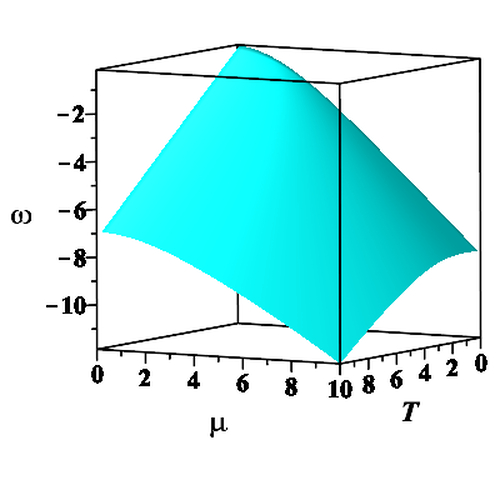
In Figs. 5, 6, the Landau and Helmholtz free energies are depicted as functions of temperature and chemical potential. For low temperatures and high values of the chemical potential, one can observe a slightly pronounced minimum in the behavior of the Helmholtz free energy and a flat Landau free energy for the Type A graph (Fig. 6).
In Figs. 7, 8 the average clustering coefficients in the whole network, are presented for different magnitudes of the chemical potential. For high temperatures, both clustering coefficients behave according to the theoretical predictions, . However, for low temperatures, the results are quite different. For Type B graphs, both definitions lead to the clustering coefficient’s correct behavior in the limit of the low -regime: when .
The low density of the graph characterizes type A in the limit of low temperatures and , i.e., as . Therefore, one expects the clustering coefficient to behave in the same way, as . While the first definition yields the wrong result, when , the behavior of is in agreement with the behavior of the average node degree (Fig. 4).
Our numerical simulations are confirmed by Appendix A’s analytical results, where the comparison between the two measures is made. We show that in a low-temperature regime, the clustering coefficients behave as
| (82) | ||||
| (83) |
Based on these findings, we will use the definition of for the global clustering coefficient.
III.1 Phase transitions in asymptotically sparse networks
We are interested in the asymptotically sparse network model with large number of nodes, , and vanishing average node degree in the range of temperature . Since , we will replace by in all formulas having this factor. We consider a particular model with the chemical potential defined as , where is a temperature-independent parameter Krioukov et al. 2009; Krioukov et al. 2010; Nesterov and Mata Villafuerte 2020. As follows from our previous analysis, the chemical potential should be infinite at .
To determine , we use the relation . After substitution of in Eq. (77), we obtain
| (84) |
where we use the relation Prudnikov et al. 2002
| (85) |
to replace the second term in Eq. (77). Here
| (86) |
and denotes the digamma function Frank W. J. Olver 2010.
We make use of the asymptotic properties of the generalized hypergeometric functions A. et al. 1953; Frank W. J. Olver 2010; Abramowitz and Stegun 1965 to get
| (87) |
As seen, the asymptotic series converges when . Still supposing and, in addition, assuming that when , we obtain
| (88) |
For high temperatures, , similar consideration yields
| (89) |
Substituting and taking the limit of , we get
| (90) |
Now that we have obtained the constant , we can find the dependence of the chemical potential on temperature for Type A and Type B networks employing Eqs. (77), (80). We obtain
| (91) |
where is the expected number of links. (Hereafter we omit the subindices in all calculations.)
Since an analytical solution of this equation does not exist, we solve it numerically. In Fig. 9 the chemical potential for Type A (blue curve) and Type B (red curve) networks is depicted. For the Type A graph we have as . The Type B network’s chemical potential is a continuous and bounded function of temperature and for both networks when .

In Fig. 10 the average node degree per node, , is presented. For both graphs, when , as expected. However, the average node degree’s behavior for Type A and Type B graphs is highly different for low temperatures. While is a smooth function of temperature for the Type B graph, for the Type A graph, this is not true. At the point , the system experiences a phase transition. Below the critical temperature, the graph is completely disconnected, . In Fig. 11 the Landau and Helmholtz free energies of Type A graphs are depicted. Both energies are continuous functions of temperature; however, they lost their analytical properties at the critical point .
Near the critical temperature the chemical potential behaves as
| (92) |
where is the reduced temperature. The constant, , is calculated by performing the numerical simulations (see SM for details). We obtain
To describe the phase transition, we introduce the order parameter, , which ranges between zero and one. We find that near the critical temperature the thermodynamic potentials behave as (see SM for details)
| (95) | ||||
| (96) | ||||
| (97) | ||||
| (98) | ||||
| (99) |
where
| (100) |
Next, substituting in Eqs. (196) – (164), we obtain the dependence of the thermodynamic potentials on the average node degree in the whole network
| (101) | ||||
| (102) | ||||
| (103) | ||||
| (104) | ||||
| (105) |
Finally, employing Eq. (179) and keeping the leading terms in Eqs.(101) – (105), one can obtain the dependence of thermodynamic functions on the reduced temperature. In Table I, we summarize our results.
Table I. Critical exponents for
| Thermodynamic functions | Relation |
|---|---|
| Chemical potential | |
| Order parameter | |
| Landau free energy | |
| Helmholtz free energy | |
| Internal energy | |
| Entropy | |
| Heat capacity |
III.2 Degree distribution
We are now ready to analyze the topological properties of the network. First, we are interested in the degree distribution, . To proceed, we use generating functions approach presented in Sec. II. The generating function for sparse networks is given by Eq. (49), written as
| (106) |
where is the expected degree of the node with the hidden variable (see Eq. (76)).
The computation of the degree distribution yields
| (107) |

In Fig. 12 the degree distribution, , is depicted as a function of and temperature. With increasing temperature, the dependence of on is changed from power-degree, for lower temperatures, to a Poisson-like distribution for high temperatures. To prove this conjecture, below we will consider two limited cases, and , and derive the approximate formulas for their degree distribution.
Low temperatures
Near the critical temperature, taking into account that , we obtain
| (108) | ||||
| (109) | ||||
| (110) |
As one can see, the main contribution in computation of integrals (106), (107) yield high energies, . Using the asymptotic properties of the hypergeometric functions Abramowitz and Stegun 1965; Frank W. J. Olver 2010, we obtain
| (111) | ||||
| (112) |
where . Note that at the critical point .
Using these results, we rewrite Eq. (106) as
| (113) |
where and . Performing the integration, we obtain
| (114) |
where . To verify our results, we derive and . We find that and , as expected.
In order to get the degree distribution, we use expression (113) for the generating function. Taking the derivatives at the point , we find
| (115) |
Performing the integration, we obtain
| (116) |
where we have used Eq. (45) in computing the degree distribution.
Since , one can neglect the last term and write
| (117) |
Thus, near the critical point the degree distribution scales as , with . At the critical point we have .
High temperatures
Now let us consider the case of high temperatures, . Proceeding as above, we obtain
| (118) | ||||
| (119) | ||||
| (120) |
When we have , as was predicted by the model.
Now we can repeat the same procedure that we did in the case of of low temperatures (). Straightforward computation of the generating function yields
| (121) |
In the calculation of this expression we have used the asymptotic properties of the incomplete gamma function for large Frank W. J. Olver 2010. This leads to a Poisson distribution for the degree distribution:
| (122) |
Thus, we find that in the limit of high temperatures the degree distribution does not depend on , and the graph becomes a random graph. This is a universal behavior of scale-free networks.
(a)
(b)
In Fig. 13 we compare the approximate (red dashed curves) and exact (solid blue curves) expressions for the degree distribution. One can see an excellent agreement between both the approximate and exact results for low and high temperatures.
III.3 Formation of a giant component
Most real networks exhibit inhomogeneity in their link distribution leading to the natural clustering of the network into groups or communities. Within the same community, node-node connections are dense, but between groups, connections are less dense. A group of nodes forms a component when all of them are connected, directly or indirectly Newman et al. 2001; Girvan and Newman 2002.
A “giant component” contains a significant part of the total number of nodes. For instance, if the degree connection , the whole network is a giant component. In particular, this is valid for a Type B graph in the limit of . In Sec. II, we have shown that, for both dense and Type A graphs, in the limit of high temperatures. Thus, one can expect that with increasing temperature the dense network should be fragmented in a finite number of giant components, and in a sparse network, giant components should arise. In what follows, we will show that only one giant component arises in our model.
A giant component is formed in the network when the following condition holds Girvan and Newman 2002:
| (123) |
Using the relations and , one can recast (123) as
| (124) |
The computation of employing the generating function (113) yields
| (125) |
Using this in combination with Eq. (124) leads to
where is the threshold.
The structural phase transition, leading to percolation, results in the giant component emerging and occurs at the temperature , where . Employing (III.3) we find that the critical temperature , if , and when . We see that for networks with , the transition associated with percolation still exists, though at a vanishing threshold this result was reported before in Cohen et al. 2002.).
Let be the fraction of the graph occupied by the giant component. Then the size of the giant component is defined by Newman et al. 2001
| (128) |
where is the smallest non-negative real solution of the equation
| (129) |
Fig. 14 shows the giant component’s size for a network with and nodes. As one can see, the size of the giant component is a rapidly increasing function. The saturation occurs for comparatively low temperatures and values of the average node degree.
(a)
(b)
Below we study two important cases in detail: low and high temperature limits .
Low temperatures
As has been shown above, for low temperatures the generating function can be approximated as
| (130) |
where and . In the thermodynamic limit, one can neglect the last term and write
| (131) |
We now examine Eq. (129) in detail. Using the series expansion for the incomplete gamma function Frank W. J. Olver 2010,
| (132) |
we recast Eq.(129) as
| (133) |
where .
First we consider the case with . Keeping only dominant terms as , we obtain
| (134) |
For networks with we have a non-vanishing threshold, , therefore it is convenient to introduce a new small parameter, . Returning to Eq. (133) we find
| (135) |
Considering only the leading terms as , we obtain
Returning to the size of the giant component we find that . In conjunction with (134) and (III.3) this yields
To compare our results with those known for the percolation phase transitions, we use the relation
| (141) |
where , is the threshold, and denotes the fraction of nodes (and their links) removed from the network Romualdo Pastor-Satorras 2003; Cohen et al. 2002.
The size of the giant component near the critical point behaves as Romualdo Pastor-Satorras 2003. Employing Eq. (III.3) in combination with Eq. (III.3), we find that the critical exponent, , is given by
This is in agreement with the results reported in Cohen et al. 2002.
High temperatures
In this case, in order to to derive the size of the giant component, we employ Eq.(121) for the generating function,
| (145) |
Proceeding as above, we find that satisfies the functional equation:
| (146) |
In this limit , and the size of the giant component can be estimated as follows:
| (147) |
When we obtain . Thus, for , almost all nodes of the network belong to the giant component. However, since , the giant component does not fill the entire graph. Moreover, only one giant component can be formed in the network, in agreement with the known results for graphs with purely power-law distributions Newman et al. 2001.
Conclusion
We demonstrated some diverse critical effects and phenomena occurring in networks, which significantly differ from those in lattices. We have shown how to treat random and scale-free networks within the conventional statistical physics approach and elucidated the role of network temperature. The temperature is a parameter that controls the average node degree in the whole network and governs the transition from unconnected to power-degree (scale-free) and random graphs. With increasing temperature, the degree distribution is changed from power-degree, for lower temperatures, to a Poisson-like distribution for high temperatures. Temperature can act contra common sense in networks; for instance, increasing the sparse scale-free networks’ temperature results in a high connection degree. For dense networks, the opposite is valid.
We introduced a configuration network model with hidden variables and found a finite-temperature phase transition for an asymptotically sparse network. The phase transition leads to fundamental structural changes in the network topology. The low-temperature phase yields a wholly disconnected graph. Above the critical temperature, the graph becomes connected, and a giant component appears. Near the critical temperature, the size of the giant component . This implies many vertices with a low degree and a small number with a high degree in the network. For high temperatures, almost all nodes of the network belong to the giant component. However, it turns out that the giant component does not fill the entire graph, even for the network’s infinite temperature.
Our results suggest that a network temperature might be an inalienable property of real networks placing conditions on degree distribution, the topology of networks, and spreading information across these systems. We believe that our approach provides a unified statistical description of real networks’ properties, from their scale-free and random graphs behavior to community structure and topology change.
Acknowledgements.
The authors acknowledge the support by the CONACYT.Appendix A Clustering coefficients
In this Appendix, we obtain the analytic expressions for the global clustering coefficients for type A networks in the limit of low temperatures, . We assume that the chemical potential . The small parameters in the asymptotic expansions been used are: and . As one can see , therefore, when it is applied, we keep the term and omit .
The global clustering coefficients, , are given by
| (148) | ||||
| (149) |
where , ,
| (150) |
and so on.
It is convenient to introduce a new variable and recast (148) and (149), as
| (151) | ||||
| (152) |
where , and
| (153) |
In Eqs. (151) and (152), we set
| (154) | ||||
| (155) |
| (156) | ||||
| (157) |
The computation of in the low-temperature limit yields . Next, substituting in (154), we obtain . The computation of in the low-temperature limit yields . Next, substituting in (154), we obtain . To calculate we take into account that the leading term is obtained when . Then taking the integral (157), we obtain
| (158) |
Substitution of in (156) yields
| (159) |
The computation of the integral with help of the formula from the table of integrals Prudnikov et al. 2002,
| (160) |
where
| (161) | ||||
| (162) |
yields
| (163) |
Global clustering coefficient
In the low-temperature regime, the clustering coefficient’s behavior is described by the following Proposition.
Proposition 1.
In the low-temperature limit, , the global clustering coefficient behaves as
where .
Proof.
The leading contribution in is determined by
| (164) |
Substitution of and yields
| (165) |
where
| (166) |
Making a change of variables, , we obtain
| (167) |
To proceed further we employ the formula from the table of integrals Prudnikov et al. 2002
| (168) |
where
| (169) |
and denotes the digamma function Frank W. J. Olver 2010. The computation yields
| (170) |
Substitution of this result in (165) yields
| (171) |
∎
Global clustering coefficient
In the low temperature regime, the clustering coefficient’s behavior is described by the following Proposition.
Proposition 2.
In the low-temperature limit, the global clustering coefficient behaves as
where .
Proof.
Substituting and in Eq. (152), we obtain
| (172) |
where and
| (173) |
The leading contribution in is determined by the term , where
| (174) |
The limit exists, since as . Using this result, we obtain
| (175) |
Thus, in low-temperature regime
| (176) |
∎
Appendix B Supplementary Material
In the Supplementary Material (SM), we calculate the critical exponent and find the logarithmic corrections to the leading power laws that govern the order parameter and thermodynamic potentials as a phase transition point is approached. First, we consider the behavior of the chemical potential near the critical temperature. The dependence of the chemical potential on temperature is defined by the equation, , where is the expected number of links. Assuming and substituting in the equation,
| (177) |
we obtain
| (178) |
The solution of this equation yields the chemical potential as a function of temperature.
To describe the behavior of the chemical potential near the critical point, we use the trial function
| (179) |
where is the reduced temperature, and is a fitting constant. As shown in Fig.15, formula (179) approximates the exact solution of the Eq. (178) well, with the choice of being
Further it is convenient to introduce a new function . Now we can find as a limit of , when , i.e. . After the substitution in Eq. (178), it becomes the equation that implicitly defines the dependence of the function on temperature. In Fig. 16 we compare the results of our numerical solution of Eq. (178) obtained for with the critical exponent given by Eq. (B). One can see a good agreement between both the approximate and exact results.
The critical exponent associated with the order parameter, , is defined as
| (182) |
In our model the order parameter is determined by the chemical potential, . Substituting from Eq. (179), we find , where the critical exponent, , is given by Eq. (B).
To obtain the Landau free energy dependence on the order parameter, we start with the exact expression for .
| (183) |
Near the critical point one can approximate it as
| (184) |
where ,
| (185) |
In derivation of Eq. (190) we use the relation A. et al. 1953; Frank W. J. Olver 2010; Abramowitz and Stegun 1965; Prudnikov et al. 2002,
to replace the Lerch transcendent by the hypergeometric function .
To proceed further, we use the linear transformation formulas of the hypergeometric function, yielding
| (188) |
For we get
| (189) |
and after substituting (189) in Eq.(190) with , we obtain
| (190) |
The limiting case with being integer, , can be covered by using the linear transformation of variables Abramowitz and Stegun 1965
| (191) |
followed by the hypergeometric series A. et al. 1953
| (192) |
where and
| (193) |
The computation yields
| (194) |
where , and denotes the Psi-function Frank W. J. Olver 2010. Using (194) in Eq.(190) we obtain
| (195) |
References
- Bollobás (2001) B. Bollobás, Random Graphs (Cambridge University Press, Cambridge, 2001).
- S. N. Dorogovtsev and J. F. F. Mendes (2003) S. N. Dorogovtsev and J. F. F. Mendes, Evolution of Networks: From Biological Nets to the Internet and WWW (Oxford University Press, Oxford, 2003).
- Caldarelli (2007) G. Caldarelli, Scale-Free Networks: Complex Webs in Nature, and Technology (Oxford University Press, Oxford, 2007).
- Barrat et al. (2008) A. Barrat, M. Barthelemy, and A. Vespignani, Dynamical Processes on Complex Networks (Cambridge University Press, Cambridge, 2008).
- Barabási (2016) A.-L. Barabási, Network Science (Cambridge University Press, Cambridge, 2016).
- Newman (2018) M. Newman, Networks (Oxford University Press, Oxford, 2018).
- Albert and Barabási (2002) R. Albert and A.-L. Barabási, “Statistical mechanics of complex networks,” Rev. Mod. Phys. 74, 47–97 (2002).
- Watts and Strogatz (1998) Duncan J. Watts and Steven H. Strogatz, “Collective dynamics of ‘small-world’ networks,” Nature 393, 440 – 442 (1998).
- Kwapień and Drozdz (2012) J. Kwapień and S. Drozdz, “Physical approach to complex systems,” Physics Reports 515, 115 – 226 (2012).
- Barabási (2009) Albert-László Barabási, “Scale-free networks: A decade and beyond,” Science 325, 412–413 (2009).
- Girvan and Newman (2002) M. Girvan and M. E. J. Newman, “Community structure in social and biological networks,” Proceedings of the National Academy of Sciences 99, 7821–7826 (2002).
- Voitalov et al. (2019) I. Voitalov, P. van der Hoorn, R. van der Hofstad, and Dmitri Krioukov, “Scale-free networks well done,” Phys. Rev. Research 1, 033034 (2019).
- Newman et al. (2001) M. E. J. Newman, S. H. Strogatz, and D. J. Watts, “Random graphs with arbitrary degree distributions and their applications,” Phys. Rev. E 64, 026118 (2001).
- Newman (2003) M. E. J. Newman, “The structure and function of complex networks,” SIAM Review 45, 167–256 (2003).
- Romualdo Pastor-Satorras (2003) A. Diaz-Guilera (eds.) R. Pastor-Satorras, M. Rubi, Statistical Mechanics of Complex Networks, Lecture Notes in Physics 625 (Springer-Verlag, New York, 2003).
- Park and Newman (2004) J. Park and M. E. J. Newman, “Statistical mechanics of networks,” Phys. Rev. E 70, 066117 (2004).
- Garlaschelli and Loffredo (2008) D. Garlaschelli and M. I. Loffredo, “Maximum likelihood: Extracting unbiased information from complex networks,” Phys. Rev. E 78, 015101(R) (2008).
- Cimini et al. (2019) G. Cimini, T. Squartini, F. Saracco, D. Garlaschelli, A. Gabrielli, and G. Caldarelli, “The statistical physics of real-world networks,” Nature Reviews Physics 1, 58–71 (2019).
- Mikulecky (2001) D. C. Mikulecky, “Network thermodynamics and complexity: a transition to relational systems theory,” Computers Chemistry 25, 369 – 391 (2001).
- Garlaschelli et al. (2013) D. Garlaschelli, S. E. Ahnert, T. M. A. Fink, and G. Caldarelli, “Low-temperature behaviour of social and economic networks,” Entropy 15, 3148–3169 (2013).
- Krioukov et al. (2009) D. Krioukov, F. Papadopoulos, A. Vahdat, and M. Boguñá, “Curvature and temperature of complex networks,” Phys. Rev. E 80, 035101(R) (2009).
- Krioukov et al. (2010) D. Krioukov, F. Papadopoulos, M. Kitsak, A. Vahdat, and M. Boguñá, “Hyperbolic geometry of complex networks,” Phys. Rev. E 82, 036106 (2010).
- Nesterov and Mata Villafuerte (2020) A. I. Nesterov and P. H. Mata Villafuerte, “Complex networks in the framework of nonassociative geometry,” Phys. Rev. E 101, 032302 (2020).
- Callaway et al. (2000) D. S. Callaway, M. E. J. Newman, S. H. Strogatz, and Duncan J. Watts, “Network robustness and fragility: Percolation on random graphs,” Phys. Rev. Lett. 85, 5468–5471 (2000).
- Dorogovtsev et al. (2008) S. N. Dorogovtsev, A. V. Goltsev, and J. F. F. Mendes, “Critical phenomena in complex networks,” Rev. Mod. Phys. 80, 1275–1335 (2008).
- Boguñá and Pastor-Satorras (2003) M. Boguñá and R. Pastor-Satorras, “Class of correlated random networks with hidden variables,” Phys. Rev. E 68, 036112 (2003).
- Serrano et al. (2008) M. Á. Serrano, D. Krioukov, and Marián Boguñá, “Self-similarity of complex networks and hidden metric spaces,” Phys. Rev. Lett. 100, 078701 (2008).
- Boccaletti et al. (2006) S. Boccaletti, V. Latora, Y. Moreno, M. Chavez, and D.-U. Hwang, “Complex networks: Structure and dynamics,” Physics Reports 424, 175 – 308 (2006).
- Squartini and Garlaschelli (2017) T. Squartini and D. Garlaschelli, Maximum-Entropy Networks: Pattern Detection, Network Reconstruction and Graph Combinatorics (Springer International Publishing, Cham, 2017).
- van der Hoorn et al. (2018) P. van der Hoorn, G. Lippner, and D. Krioukov, “Sparse Maximum-Entropy Random Graphs with a Given Power-Law Degree Distribution,” Journal of Statistical Physics 173, 806–844 (2018).
- Anand et al. (2014) K. Anand, D. Krioukov, and G. Bianconi, “Entropy distribution and condensation in random networks with a given degree distribution,” Phys. Rev. E 89, 062807 (2014).
- Voitalov et al. (2020) I. Voitalov, P. van der Hoorn, M. Kitsak, F. Papadopoulos, and D. Krioukov, “Weighted hypersoft configuration model,” Phys. Rev. Research 2, 043157 (2020).
- Barrat and Weigt (2000) A. Barrat and M. Weigt, “On the properties of small-world network models,” The European Physical Journal B - Condensed Matter and Complex Systems 13, 547–560 (2000).
- Bollobás and Riordan (2003) B. Bollobás and O. M. Riordan, “Mathematical results on scale-free random graphs,” in Handbook of graphs and networks: from the genome to the Internet, edited by Stefan Bornholdt and Heinz Georg Schuster (Wiley-VCH, Weinheim, 2003).
- Wilf (2006) H. S. Wilf, Generatingfunctionology, 3rd ed. (A K Peters, Wellesley, MA, 2006).
- Chung and Lu (2002a) F. Chung and L. Lu, “Connected Components in Random Graphs with Given Expected Degree Sequences,” Annals of Combinatorics 6, 125–145 (2002a).
- Chung and Lu (2002b) F. Chung and Linyuan Lu, “The average distances in random graphs with given expected degrees,” Proceedings of the National Academy of Sciences 99, 15879 (2002b).
- Caldarelli et al. (2002) G. Caldarelli, A. Capocci, P. De Los Rios, and M. A. Muñoz, “Scale-free networks from varying vertex intrinsic fitness,” Phys. Rev. Lett. 89, 258702 (2002).
- Servedio et al. (2004) V. D. P. Servedio, G. Caldarelli, and P. Buttà, “Vertex intrinsic fitness: How to produce arbitrary scale-free networks,” Phys. Rev. E 70, 056126(R) (2004).
- Squartini and Garlaschelli (2011) T. Squartini and D. Garlaschelli, “Analytical maximum-likelihood method to detect patterns in real networks,” New Journal of Physics 13, 083001 (2011).
- Park and Newman (2003) J. Park and M. E. J. Newman, “Origin of degree correlations in the Internet and other networks,” Phys. Rev. E 68, 026112 (2003).
- Frank W. J. Olver (2010) R. F. Boisvert, C. W. Clark, F. W. J. Olver, D. W. Lozier, NIST Handbook of Mathematical Functions (Cambridge University Press, Cambridge, 2010).
- A. et al. (1953) E. A., Magnus W., and Oberhettinger F., Higher Transcendental Functions, Vol. I. (McGraw-Hill, New York, NY, USA, 1953).
- Prudnikov et al. (2002) A. P. Prudnikov, Yu. A. Brychkov, and O. I. Marichev, Integrals and series. 3, More special functions (Gordon and Breach Science Publishers, 2002).
- Abramowitz and Stegun (1965) M. Abramowitz and I. A. Stegun, eds., Handbook of Mathematical Functions (Dover, New York, 1965).
- Cohen et al. (2002) R. Cohen, D. ben-Avraham, and S. Havlin, “Percolation critical exponents in scale-free networks,” Phys. Rev. E 66, 036113 (2002).
- Prudnikov et al. (2002) A. P. Prudnikov, Yu. A. Brychkov, O. I. Marichev, and N. M. Queen (Translator), Integrals and Series: elementary functions (CRC, 1998).