A parallel structured divide-and-conquer algorithm for symmetric tridiagonal eigenvalue problems
Abstract
In this paper, a parallel structured divide-and-conquer (PSDC) eigensolver is proposed for symmetric tridiagonal matrices based on ScaLAPACK and a parallel structured matrix multiplication algorithm, called PSMMA. Computing the eigenvectors via matrix-matrix multiplications is the most computationally expensive part of the divide-and-conquer algorithm, and one of the matrices involved in such multiplications is a rank-structured Cauchy-like matrix. By exploiting this particular property, PSMMA constructs the local matrices by using generators of Cauchy-like matrices without any communication, and further reduces the computation costs by using a structured low-rank approximation algorithm. Thus, both the communication and computation costs are reduced. Experimental results show that both PSMMA and PSDC are highly scalable and scale to 4096 processes at least. PSDC has better scalability than PHDC that was proposed in [J. Comput. Appl. Math. 344 (2018) 512–520] and only scaled to 300 processes for the same matrices. Comparing with PDSTEDC in ScaLAPACK, PSDC is always faster and achieves x–x speedup for some matrices with few deflations. PSDC is also comparable with ELPA, with PSDC being faster than ELPA when using few processes and a little slower when using many processes.
Index Terms:
PSMMA, PUMMA Algorithm, ScaLAPACK, Divide-and-conquer, Rank-structured matrix, Cauchy-like matrixI Introduction
Computing the eigendecomposition of a symmetric tridiagonal matrix is an important linear algebra problem and is widely used in many fields of science and engineering. It is usually solved by divide-and-conquer (DC) [1, 2], QR [3], MRRR [4, 5], and some other methods. The DC algorithm is now the default method in LAPACK [6] and ScaLAPACK [7] when the eigenvectors are required. DC is usually very efficient in practice, requiring only flops for matrices with dimension on average [8], but its complexity can still be for some matrices with few deflations. The performance of an algorithm not only depends on the number of floating point operations, but also other ingredients such as communication and data movements, etc. Some communication-avoiding algorithms have been developed recently [9, 10]. In this work, we aim to accelerate the parallel DC algorithm on distributed memory machines by reducing both the computation complexity and communication complexity. Our algorithm can be much faster than the ScaLAPACK routine PDSTEDC for those difficult matrices, and can scale to thousands of processes. Experimental results are included in section IV.
It is known that some Cauchy-like matrices with off-diagonally low-rank properties appear in the DC algorithm [1, 2], which can be approximated by hierarchically semiseparable (HSS) matrices [11, 12]. Then, the worst case complexity of DC can be reduced from to , where is a modest number and is usually much smaller than a large , see [13]. This technique was extended for the bidiagonal and banded DC algorithms for the SVD problem on a shared memory multicore platform in [14, 15]. For distributed memory machines, a parallel DC algorithm is similarly proposed in [16] by using STRUMPACK (STRUctured Matrices PACKage) [17], which provides some distributed parallel HSS algorithms. The accelerated DC proposed in [16] was called PHDC. However, numerical results show that for the simple matrix-matrix multiplication operations, STRUMPACK is not as scalable as PDGEMM, and may become slower than PDGEMM when using 300 or more processes on Tianhe-2 supercomputer. See [16] for details.
Instead of using HSS, this work exploits a much simpler type of rank-structured matrix, called BLR (Block low-rank format [18]). Compared with HSS, BLR abandons the hierarchy but compresses the off-diagonal blocks. It loses the near-linear complexity of other hierarchical matrices such as -matrix [19], -matrix [20], and HSS matrix. Because of its simple structure, BLR is easy to implement in parallel, and often improves the scalability of corresponding algorithms, see [18, 21] for more details.
In this paper, we propose a parallel structured matrix-matrix multiplication algorithm for Cauchy-like matrices, which will be named PSMMA. It exploits the off-diagonal low-rank property of matrices like BLR, and it can further reduce the communication cost by constructing local submatrices using the generators, which will be explained in section III. Our main contributions include the following:
- •
We propose a parallel structured matrix multiplication algorithm (PSMMA) for structured matrices including Cauchy-like, Toeplitz, Hankel, Vandermonde, etc. PSMMA can reduce both the communication and computation costs by using low-rank approximations. To the best of the authors’ knowledge, none of the matrix multiplication algorithms has been developed to reduce the communication cost by exploiting the structure of matrices.
- •
PSMMA works for matrices both in the block cyclic data distribution (BCDD) form (like ScaLAPACK) and block data distribution (BDD) form (2D block partitioning). It also works for general process grids.
- •
Combining PSMMA with the DC algorithm in ScaLAPACK, we propose a parallel structured DC algorithm (PSDC), which can be much faster than PDSTEDC in ScaLAPACK. PSDC is also competitive with ELPA [22].
The process of PSMMA is similar to Cannon [23] and Fox [24] algorithms. However, PSMMA works for matrices in BCDD form and works for any rectangular process grids. From this perspective, PSMMA is more like PUMMA [25], a generalized Fox algorithm. PSMMA is more efficient than PUMMA for structured matrices and details are shown in section III-A2. It has three advantages compared with PUMMA. One advantage is that PSMMA constructs the required submatrix locally by using the generators without communication and thus requires less communication. Another one is that PSMMA combines with low-rank approximations and therefore the computation complexity is also reduced. The third one is that PSMMA requires less workspace and the size of local matrix multiplications is also larger than PUMMA. In this paper, SRRSC [14, 26] is used to compute the low-rank approximations of Cauchy-like matrices in PSMMA, which only requires linear storage. Note that PDGEMM implements an algorithm similar to SUMMA [27]. Compared with SUMMA [27], which is based on the outer product form of matrix multiplication, PSMMA can naturally exploit the off-diagonal low-rank property of matrices.
By incorporating PSMMA into the DC algorithm in ScaLAPACK [8], we obtain a highly scalable DC algorithm, which has much better scalability than the previous PHDC algorithm [16]. To distinguish from PHDC, we call the newly proposed algorithm parallel structured DC algorithm (PSDC). Numerical results show that PSDC is always faster than PDSTEDC in ScaLAPACK, and scales to 4096 processes at least. That is because PSDC requires both less computations and communications than PDSTEDC. The speedups of PSDC over PDSTEDC can be up to x-x for some matrices with dimension on Tianhe-2 supercomputer. Note that PHDC in [16] can only scale to 300 processes for the same matrices.
The remaining sections of this paper are organized as follows. Section II introduces the DC algorithm, the SRRSC algorithm for constructing low-rank approximations of Cauchy-like matrices, and some classical parallel matrix multiplication algorithms. Section III presents the newly proposed parallel structured matrix multiplication algorithm PSMMA, and describes the implementation details of PSDC, which combines PSMMA with the parallel tridiagonal DC algorithm in ScaLAPACK. All the experimental results are reported in section IV, and some future works are included in section IV-B. Conclusions are drawn in section V.
II Preliminaries
Assume is a symmetric tridiagonal matrix,
| (1) |
We briefly introduce some formulae of Cuppen’s divide-and-conquer algorithm [1, 8]. The ScaLAPACK routine also implements this version of DC algorithm [8] based on rank-one update.
Firstly, is decomposed into the sum of two matrices,
| (2) |
where , is the off-diagonal element at the th row of and with ones at the th and th entries. If and , then can be written as
| (3) |
where
Since and are orthogonal matrices, the problem is reduced to computing the spectral decomposition of a diagonal plus rank-one matrix,
| (4) |
where is a diagonal matrix, is a diagonal matrix whose diagonal elements are the eigenvalues of matrix , and is the eigenvector matrix of . Then, the eigenvector matrix of is computed as
| (5) |
The eigenvalues of are the roots of the secular equation
| (6) |
where is the th diagonal entry of , is the th component of . Then, the eigenvector is computed as
| (7) |
The main observation of works [16, 13] is that
| (8) |
where , is a Cauchy-like matrix, and the vectors and are called generators.
The whole classical DC algorithm is shown in Algorithm 1. The main computational task of DC lies in computing the eigenvectors via matrix-matrix multiplications (MMM) (5), which costs flops. Since is a Cauchy-like matrix and off-diagonally low-rank, MMM (5) can be accelerated by using HSS matrix algorithms, and the computational complexity can be reduced significantly, see [16, 13] for more details. The aim of this work is not only to reduce the computation cost of MMM (5) but also its communication cost in the distributed memory environment. For simplicity, we do not consider deflation in (5). About the deflation process, we refer the interested readers to [1, 28] and section III-B.
II-A SRRSC low-rank approximation
A novel low-rank approximation method for Cauchy-like matrix is proposed in [14, 26], which only requires linear storage. For completeness, this method is introduced briefly in this section, which only works on the generators.
Assume that is an Cauchy-like matrix, . The following factorization is called the th Schur complement factorization of ,
| (9) |
where and is called the th Schur complement.
One good property of a Cauchy-like matrix is that its th Schur complement is also Cauchy-like [29, 30], and its generators can be computed recursively as follows.
Theorem 1
The th Schur complement satisfies
with and . Then
| (10) |
| (11) |
with , , and .
Corollary 1
For , the generators of are
| (12) |
| (13) |
It is easy to prove that is also Cauchy-like, and its generators can also be computed recursively.
Theorem 2
The generators of satisfy the displacement equation
where and , and
| (14) |
and are computed recursively by equation (13). Furthermore,
Since permutation does not destroy the structure of Cauchy-like matrices, we can permute generators and to make the first entry of , , large. A complete pivoting strategy could be used. Some efficient pivoting strategies have been proposed in [30] and [31]. We used the pivoting strategy proposed in [14].
If the entries of are negligible, and then by ignoring , we get a low-rank approximation to ,
| (15) |
where and is a permutation matrix which records the column permutations during the pivotings. To be more specific, consists of a subset of columns of , and from Theorem 2,
| (16) |
where is the array after permutation.
II-B Parallel Matrix-Matrix multiplications
Matrix-matrix multiplication is a very important computational kernel of many scientific applications. In this subsection, we briefly introduce some parallel matrix multiplication algorithms, which compute .
Cannon algorithm [23] was the first efficient algorithm for parallel matrix multiplication providing theoretically optimal communication cost. However it requires the process grid to be square, which limits its practical usage. Fox algorithm proposed in [24] has the same problem. The PUMMA algorithm [25] is a generalized Fox algorithm, and it works for a general processor grid. PUMMA was designed for ScaLAPACK and used the BCDD form.
The current version of ScaLAPACK implements SUMMA [27], which was proposed in the mid-1990s and designed for a general processor grid. It also uses the block-cyclic data distribution form. It implements the outer product form of matrix multiplication, and allows to pipeline them. PUMMA implements the inner product form, and requires the largest possible matrices for computations and communications. Some more efficient matrix multiplication algorithms have been proposed recently, like 2.5D algorithm [32], CARMA [33], CTF [34], and COSMA [35], and many others. Since they are not quite related to this current work, we do not attempt to give a complete literature review.
PUMMA is more appropriate for the rank-structured matrices than SUMMA, since the large off-diagonal blocks can be compressed by low-rank approximations. So are Cannon and Fox algorithms. It is not obvious for SUMMA to exploit the rank-structured property of the input matrices.
In this paper, we propose a parallel structured matrix multiplication algorithm, which is called PSMMA for short. We assume at least one of the two matrices is a structured matrix. By ’structured matrices’ we mean those matrices which can be expressed using parameters where is the dimension of matrix, e.g. Cauchy-like, Toeplitz, Hankel, and Vandermonde matrices [36]. PSMMA can be based on the BCDD structure like PUMMA and ScaLAPACK, and it can also be based on the BDD structure like Cannon or Fox algorithms. As shown later, the second approach is more efficient to exploit the off-diagonal low-rank structure. Its drawback is that it requires to redistribute the matrix from the BCDD form to BDD form, since the matrices are initially stored in BCDD form in ScaLAPACK routines. The PSMMA in BCDD form fits well with ScaLAPACK routines and does not need any data redistribution.
By exploiting the special structure of matrix, PSMMA can reduce both the computation and communication costs. To the best of the authors’ knowledge, this work is the first one proposing a reduction of the communication cost of matrix multiplication algorithms by exploiting the structures of matrices.
III Algorithm Proposed
The main contributions of this paper consist of two parts. First, we design a parallel structured matrix multiplication algorithm for structured matrices in section III-A, which is called PSMMA and can reduce both the computation and communication costs.
Secondly, section III-B shows how to combine PSMMA with the parallel tridiagonal DC algorithm in ScaLAPACK. It illustrates how to modify several routines in ScaLAPACK in order to use PSMMA. The parallel structured DC algorithm is called PSDC, and its whole procedure is summarized in Algorithm 3. A cartoon is included in Fig. 4 to show the whole workflow of PSDC.
III-A PSMMA for structured matrices
In this subsection, we introduce PSMMA to compute , where is a general matrix, is a structured matrix, and its entries can be represented by parameters. The case that is a structured matrix and is a general matrix is similar. When both and are structured matrices, all operations can be performed locally without any communication, which will be explained later. In the following sections, we assume is stored in BCDD form and is represented by its generators.
Suppose the matrix has block rows and block columns, and the matrix has block rows and block columns. Block of is then computed by
| (17) |
where . Cannon and Fox algorithms initially considered only the case of matrices in which each processor contains a single row or a single column of blocks [23, 24]. PUMMA considered the matrix multiplication algorithms with BCDD form [27]. Fig. 1 shows a block matrix stored in a process grid. It is easy to see that the matrix in the block cyclic form is obtained from the original matrix by performing row and column block permutations.

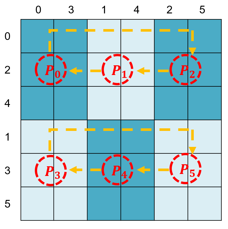
Since the matrix can be represented by its generators, any submatrices of can be formed easily. This fact enables us to treat the submatrices of in each process as a whole continuous block, and we only need to construct the proper submatrices of correctly. This is our main observation. After discovering this fact, the proposal of the PSMMA algorithm becomes very natural and simple, just following the equation (17). The whole procedure is shown in Algorithm 2.
- 1.
Each process constructs the column indexes (CIndex) of matrix based on its process column in the process grid;
- 2.
Set
- 3.
do
- (a)
For each process , construct the column indexes (RIndex) of matrix based on the process column ;
- (b)
Calculate the required subblock , and construct its low-rank approximation (if needed) by using its generators, ;
- (c)
Multiply the copied subblock with the currently residing subblock: ;
- (d)
Shift matrix leftward cyclically along each process row;
end do
- (a)
To illustrate the algorithm from the process point of view, we show how the submatrices of stored at process (located at position of the process grid) are computed for the matrix shown in Fig. 1(b). This consists of three steps, and the process is depicted in Figure 2. The column indexes of are fixed, and its row indexes are determined by the column indexes of . After each step, matrix would be shifted leftward, and the local matrix on process is updated by the matrix on process . As shown in Fig. 1(b), the local matrix of process at step is updated by that of process , which is located at the right of process . After process has received the matrix from all other processes, the algorithm stops.

Algorithm 2 works both for block cyclic data distribution and block data distribution. It only depends on the distribution of to determine the row indexes of local matrix . In step 3(b) of Algorithm 2, we construct a low rank approximation only when the local matrix is probably low rank. For the tridiagonal DC algorithm in section II, matrix is a Cauchy-like matrix and we can check whether the intersection of CIndex and RIndex is empty or not. If the intersection is empty, the submatrix is probably numerically low-rank. Otherwise, the submatrix is probably full rank. For Cauchy-like matrices, we use SRRSC discussed in section II-A to construct a low-rank approximation to matrix .
Remark 1. The PSMMA algorithm introduced in this section is also suitable for other structured matrices, such as Toeplitz, Vandermonde, and DFT (Discrete Fourier Transform) matrices. Some results will be shown in our future works.
Remark 2. Only step 3(d) of Algorithm 2 requires point-to-point communications. It can be overlapped with other computations if implemented carefully. During our numerical experiments, we did not implement this technique.
III-A1 Storage form affects the off-diagonally low-rank property
For our problem, the eigenvector matrix in equation (4) is a Cauchy-like matrix, see equation (8). It is further off-diagonally low rank, since and are interlacing. The storage form of matrix affects the low-rank property of matrix in Fig. 2. We use the following example to show the main points.
Example 0. Assume that matrix is defined as , where and are random numbers, , , , for It is known that is a rank-structured Cauchy-like matrix, see [14]. Let and assume is distributed over a process grid. Suppose that (the parameter of block size for distribution), we get the BCDD form of matrix , as shown in Fig. 3(a). By choosing , we get the BDD form of in Fig. 3(b).
Fig. 3 shows the block partitions of matrix when choosing different . The numbers in Fig. 3 are the ranks of the corresponding blocks. Fig. 3(a) shows the ranks of blocks of when is in the BCDD form. From it we can see the off-diagonal ranks in Fig. 3(a) are larger than those when is in the BDD form, which are shown in Fig. 3(b). Many flops can be saved when the ranks are small. When is initially stored in the BCDD form with small , we can transform it to the BDD form by using ScaLAPACK routine PDGEMR2D. We compare these two cases in Example 1 in section IV.


III-A2 Comparison with other algorithms
Algorithm 2 works on the whole block of local matrices, like the block partition based algorithms such as Cannon and Fox algorithms. The advantages of PSMMA over Cannon and Fox algorithms are that Algorithm 2 also works for matrices of BCDD form and also works for any rectangular process grids.
Comparing with PUMMA, which works for block cyclic data distribution and rectangular process grids, Algorithm 2 requires less workspace and the size of local matrix multiplications is larger than that in PUMMA. Based on the LCM concept, PUMMA needs extra workspace to permute the block columns of and block rows of together, which can be multiplied simultaneously. Therefore, PUMMA requires roughly as much extra workspace to store another copy of the local matrices and , which makes it impractical in real applications, see [25, 37]. Furthermore, only partial block columns (rows) can be merged together in PUMMA, while PSMMA always multiplies the whole local matrix with and it does not need to permute the block columns of or the block rows of .
Comparing with SUMMA, which is based on the outer product form of matrix multiplication, PSMMA can further exploit the low-rank structure of matrix . It is not easy for SUMMA to exploit this property.
III-B Parallel Structured DC Algorithm
The excellent performance of the DC algorithm is partially due to deflation [38, 1], which happens in two cases. If the entry of is negligible or zero, the corresponding is already an eigenpair of . Similarly, if two eigenvalues in are identical then one entry of can be transformed to zero by applying a sequence of plane rotations. All the deflated eigenvalues are moved to the end of by a permutation matrix, and so are the corresponding eigenvectors. Then, after deflation, (3) reduces to
| (18) |
where is the product of all rotations, is a permutation matrix, and are the deflated eigenvalues.
According to (4), the eigenvectors of are computed as
| (19) |
To improve efficiency, Gu [39] suggested a permutation strategy for reorganizing the data structure of the orthogonal matrices, which has been used in ScaLAPACK. The matrix in square brackets is permuted as , where the first and third block columns contain the eigenvectors that have not been affected by deflation, the fourth block column contains the deflated eigenvectors, and the second block column contains the remaining columns. Then, the computation of can be done by two parallel matrix-matrix products (calling PDGEMM) involving parts of and the matrices , . Another factor that contributes to the excellent performance of DC is that most operations can take advantage of highly optimized matrix-matrix products.
When there are few deflations, the size of matrix in (19) will be large, and most of the time spent by DC would correspond to the matrix-matrix multiplication in (19). Furthermore, it is well-known that matrix defined as in (4) is a Cauchy-like matrix with off-diagonally low rank property, see [2, 13]. Therefore, we simply use the parallel structured matrix-matrix multiplication algorithm to compute the eigenvector matrix in (19). Since PSMMA requires much fewer floating point operations and communications than the plain matrix-matrix multiplication, PDGEMM, this approach makes the DC algorithm in ScaLAPACK much faster.
As mentioned before, the central idea is to replace PDGEMM by PSMMA. The eigenvectors are updated in the ScaLAPACK routine PDLAED1, and therefore we modify it and call PSMMA in it instead of PDGEMM. The whole procedure of PSDC accelerated by PSMMA is summarized in Algorithm 3. Comparing with the classical DC algorithm (Algorithm 1), the only difference is that PSMMA is used when the size of matrix is large. In Fig. 4 the stages of PSDC are graphically represented.

Note that after applying permutations to in (19), matrix should also be permuted accordingly. From the results in [2, 13, 14], we know that is a Cauchy-like matrix and off-diagonally low-rank, the numerical rank is usually around -. When combining with PSMMA, we would not use Gu’s idea [39] since permutation may destroy the off-diagonally low-rank structure of in (19). We need to modify the ScaLAPACK routine PDLAED2, and only when the size of deflated matrix in (18) is large enough, PSMMA would be used, otherwise use Gu’s idea. In section IV, we denote the size of by , whose value depends on the matrix as well as the architecture of the particular parallel computer used, and may be different for different computers. In Example 2, PSMMA is used when .
Remark 3. To keep the orthogonality of (see equation (8)), must be computed by
| (20) |
where (the distance between and ), and (the distance between and ), which can be returned by calling the LAPACK routine DLAED4. In our implementation, is represented by using five generators, and .
IV Experimental results
All the experimental results are obtained on the Tianhe-2 supercomputer [40, 41], located in Guangzhou, China. Each compute node is equipped with two 12-cores Intel Xeon E5-2692 v2 CPUs and our experiments only use CPU cores. The details of the test platform and environment of compute nodes are shown in Table I. For all these numerical experiments, we only used plain MPI, run MPI processes per node in principle, and one process per core. For example, we used compute nodes for testing processes.
| Items | Values |
|---|---|
| 2*CPU | Intel Xeon CPU E5-2692 v2@2.2GHz |
| Memory size | 64GB (DDR3) |
| Operating System | Linux 3.10.0 |
| Complier | Intel ifort 2013_sp1.2.144 |
| Optimization | -O3 -mavx |
Example 1. Assume that is a random matrix and is defined as , where and are random numbers, , , , for It is known that is a rank-structured Cauchy-like matrix, see [14, 13]. We compute . Let , and , respectively, and choose different number of processes, , , , and , to compare PDGEMM with PSMMA. To avoid performance variance during multiple executions, we evaluated the performance of PDGEMM and PSMMA twice in the same program and called that program three times, and chose the best results among these six executions. Our codes will be released on Github (available at https://github.com/shengguolsg/PSMMA).
It is well-known that the performance of PDGEMM depends on the block size . We tested the performances of PDGEMM by choosing , and , and we found that their differences are very small. But they are better than choosing . Therefore, we chose and , which corresponds to the BCDD form and BDD form, respectively. Note that a large is better for PSMMA since the ranks of off-diagonal blocks after permutations may be smaller, see Table II.
As shown in section III-A1, we can redistribute matrix from BCDD to BDD to exploit the off-diagonal low-rank property of matrix . In this example, we tested four versions of PSMMA, which are
- •
PSMMA_BCDD: and with low-rank approximation;
- •
PSMMA_BDD: and with low-rank approximation;
- •
PSMMA_WRedist: and with data redistribution and low-rank approximation (matrix is transformed from BCDD to BDD with and then back);
- •
PSMMA_NLowrank: and without low-rank approximation;
The speedups of PSMMA over PDGEMM are shown in Fig. 5(a), 5(b) and 5(c) with dimensions , , , respectively. From the results, we can see that PSMMA_BCDD is always faster than PDGEMM except for . It is because the ranks of blocks are very large when using the BCDD form, and most of the time is spent in computing the low-rank approximations. Table II shows the ranks of the off-diagonal blocks in the first block column, see Fig. 3 for the structure of matrix . Without using low-rank approximation, PSMMA can be faster than PDGEMM. It is interesting to see that PSMMA_NLowrank is always faster than PDGEMM for these three matrices. Note that PSMMA_NLowrank requires more floating point operations than PDGEMM since it needs to construct the local submatrices. However, PSMMA_NLowrank requires fewer communications than PDGEMM.
PSMMA_WRedist is only slower than PDGEMM when the size of the matrix is small and the number of processes is large. From the last row of Table II, we can see that the ranks of off-diagonal submatrices in BDD form are much smaller than the sizes of submatrices. PSMMA_WRedist is generally faster than both PSMMA_BCDD and PSMMA_NLowrank. The disadvantage of PSMMA_WRedist is that it requires to perform data redistribution (communication). When the number of processes is large, the data redistribution represents a large portion of the overall time. Fig. 6 shows the percentages of transforming matrix from BCDD to BDD and transforming it back. It takes over of total time when is small and is large.
PSMMA_BDD is always the best and can be more than ten times faster than PDGEMM. This is because it assumes that matrix is initially stored in BDD form and the low-rank property of matrix is not destroyed either.
It is difficult to know exactly why the speedups of PSMMA_WRedist and PSMMA_BDD over PDGEMM firstly increase and then decrease. It depends on the properties of these two algorithms. Comparing with PDGEMM, PSMMA_BDD and PSMMA_WRedist save both computations and communications. When the number of processes increases, these two contributions make the speedups first increase. As the number of processes increases, the size of the local submatrix located on each process decreases, and therefore the percentage of floating point operations saved from using low-rank approximations decreases. Since PSMMA_BDD does not save many floating point operations compared to PDGEMM, the speedups decrease when using more processes. For PSMMA_WRedist, the cost of data redistribution also increases as the number of processes increases. Meanwhile, as the number of processes grows, the percentage of saved communication by PSMMA_BDD and PSMMA_WRedist increases. Therefore, PSMMA_BDD can be always faster than PDGEMM since it not only reduces computations but also communications. It is better to use PSMMA_NLowrank instead of PSMMA_WRedist when the number of processes is very large.
Remark 4. We can adaptively choose a particular PSMMA algorithm based on the size of matrix and the number of processes. It is better to use PSMMA_WRedist when the number of processes is small, and use PSMMA_BCDD or PSMMA_NLowrank when the number of processes is large and/or the size of matrix is small. It is always best to use PSMMA_BDD when it is available and matrix is off-diagonally low rank.


Example 2. We use some ’difficult’ matrices [42] for the DC algorithm, for which few or no eigenvalues are deflated. Examples include the Clement-type, Hermite-type and Toeplitz-type matrices, which are defined as follows.
The Hermite-type matrix is given as [42],
The Toeplitz-type matrix is defined as [42],
For the results of strong scaling, we let the dimension be , and use rank-structured techniques only when the size of the secular equation is larger than . We used PSMMA_WRedist and chose The results for strong scaling of PSDC are shown in Fig. 7(a). The speedups of PSDC over ScaLAPACK are reported in Fig. 7(b). We can see that PSDC is about x–x times faster than PDSTEDC in ScaLAPACK for all cases. Because of deflations, the performances of these three matrices can be different even though they have the same dimensions.


The orthogonality of the eigenvectors computed by PSDC is in the same order as those by ScaLAPACK, as shown in Table III. The orthogonality of matrix is defined as , where is the maximum absolute value of entries of . We confirm that the residuals of eigenpairs computed by PSDC are in the same order as those computed by ScaLAPACK though the results are not included here.
| Matrix | Number of Processes | |||
|---|---|---|---|---|
| Clement | - | - | - | - |
| Hermite | - | - | - | - |
| Toeplitz | - | - | - | - |
Furthermore, we compare PSDC with PHDC which was introduced in [16] and used STRUMPACK to accelerate the matrix-matrix multiplications. The results are shown in Fig. 8. For these three matrices, PSDC is much faster than PHDC when using many processes. It is better to use STRUMPACK when using few processes since HSS-based multiplications can save more floating point operations than BLR-based multiplications.

IV-A Results from real applications
In this subsection, we use three matrices that come from real applications to test PSDC. One comes from the spherical harmonic transform (SHT) [43], which has been used in [16]. One symmetric tridiagonal matrix is defined as follows, which will be denoted by SHT,
| (21) |
for , where ,
for We assume the dimension of this matrix is and .
The other two are sparse matrices obtained from the SuiteSparse matrix collection [44], called SiO and Si5H12. We first reduce each matrix into its tridiagonal form by calling ScaLAPACK routines and then call PSDC to compute its eigendecomposition. It is also the general process for computing the eigenvalue decomposition of any symmetric (sparse) matrices. These matrices are real and symmetric and their dimensions are and , respectively.
Example 3. We use matrices SHT, SiO and Si5H12 to compare PSDC with PDSTEDC. In this example, we use the rank-structured techniques, i.e. calling PSMMA, whenever the size of the secular equation is larger than , since the largest for matrix Si5H12 is when . The speedups of PSDC over PDSTEDC are reported in Table IV. The backward errors of the computed eigenpairs are also included in the third column, which are computed as
| (22) |
where is orthogonal, is diagonal with the eigenvalues as its diagonal elements, denotes the maximum Frobenius norm of each column of and denotes the 2-norm of , its largest singular value.
| Matrix | Residual | Number of Processes | ||||
|---|---|---|---|---|---|---|
| SHT | e- | 1.20 | 1.48 | 1.42 | 1.41 | |
| Si5H12 | e- | 1.27 | 1.16 | 1.15 | 1.05 | |
| SiO | e- | 1.46 | 1.31 | 1.10 | 1.15 | |
Example 4. It is known that ELPA (Eigenvalue soLver for Petascale Applications [22, 45]) has better scalability and is faster than the MKL version of ScaLAPACK. As opposed to ScaLAPACK, ELPA routines do not rely on BLACS and PBLAS, and it can overlap the computations with communications, and the computation is also optimized by using OpenMP and even GPU. For the tridiagonal eigensolver, ELPA rewrites the DC algorithm and implements its own matrix-matrix multiplications and does not use the PBLAS routine PDGEMM. In contrast, PSDC follows the main procedure of PDSTEDC, and only uses PSMMA to accelerate the expensive matrix-matrix multiplication part.
We compare PSDC with ELPA and find that it competes with ELPA (with version 2018.11.001). We use the Clement matrix to do experiments. Fig. 9 shows the execution times of PSDC and ELPA when using different processes. It shows that PSDC is faster than ELPA when using few processes, but PSDC becomes slower when using more than processes. It is because matrix multiplication is no longer the dominant factor when using many processes. It is shown in [16] that the percentage of time dedicated to the matrix multiplications can be less than 10% of the total time. The gains of ELPA are obtained from other optimization techniques.

IV-B Future works
We discuss some bottlenecks of current implementation and future works in this subsection. A restriction of our current codes is that PSMMA was only used at the top level of the DC tree. It should be used at any level as long as the size of the matrix is large. This will be modified in the near future. We did not use OpenMP or vectorization to optimize our routines. The routines for constructing the local submatrices from generators can be optimized by using vectorization and OpenMP.
Following our current work, there are some interesting research projects to do in the future. First, PSMMA can be used to extend the banded DC algorithms proposed in [15, 46] to distributed memory platforms in a similar manner. Secondly, the structured matrix-matrix multiplication techniques can be used in heterogeneous architectures, which can reduce the data movements from CPU to the accelerators such as GPU11 1 The authors would like to thank the referee for pointing out this research direction.. We only need to transform the generators to GPUs once instead of many submatrices. Last but not least, PSMMA can be adapted for Toeplitz, Hankel, DFT (Discrete Fourier Transform) and other structured matrices [47]. Some results will be included in our future works.
V Conclusions
The starting point of this paper is trying to accelerate the tridiagonal DC algorithm implemented in ScaLAPACK [8] for some difficult matrices. It is known that the main task lies in multiplying a general matrix with a rank-structured Cauchy-like matrix, see [1, 2, 13]. The main contribution of this paper is that a highly scalable parallel matrix multiplication algorithm is proposed for rank-structured Cauchy-like matrices, which fits well for the parallel tridiagonal DC algorithm.
The matrix multiplication problem is known to be very compute intensive. However, as HPC moves towards exascale computing, the development of communication-avoiding or communication-decreasing algorithms becomes more and more important. By taking advantage of the particular structures of Cauchy-like matrices, we proposed a parallel structured matrix multiplication algorithm PSMMA, which can reduce both computation and communication costs. The workflow of PSMMA is similar to PUMMA [27] and further exploits the rank-structured property of input matrices. Experimental results show that PSMMA can be much faster than PDGEMM for rank-structured Cauchy-like matrices, and the speedups over PDGEMM can be up to .
By combing PSMMA with the parallel tridiagonal DC algorithm, we propose a parallel structured DC algorithm (PSDC). For these difficult matrices for which DC deflates very few eigenvalues, PSDC is always much faster than the classical DC algorithm implemented in ScaLAPACK. Unlike PHDC which is proposed in [16], PSDC does not have scalability problem and it can scale to 4096 processes at least.
Acknowledgments
The authors would like to thank the referees for their valuable comments which greatly improve the presentation of this paper. This work is supported by National Natural Science Foundation of China (No. NNW2019ZT6-B20, NNW2019ZT6-B21, NNW2019ZT5-A10, U1611261, 61872392 and U1811461), National Key RD Program of China (2018YFB0204303), NSF of Hunan (No. 2019JJ40339), NSF of NUDT (No. ZK18-03-01), Guangdong Natural Science Foundation (2018B030312002), and the Program for Guangdong Introducing Innovative and Entrepreneurial Teams under Grant (No. 2016ZT06D211). Jose E. Roman was supported by the Spanish Agencia Estatal de Investigación (AEI) under project SLEPc-DA (PID2019-107379RB-I00).
References
- [1] J. J. M. Cuppen, “A divide and conquer method for the symmetric tridiagonal eigenproblem,” Numer. Math., vol. 36, pp. 177–195, 1981.
- [2] M. Gu and S. C. Eisenstat, “A divide-and-conquer algorithm for the symmetric tridiagonal eigenproblem,” SIAM J. Matrix Anal. Appl., vol. 16, pp. 172–191, 1995.
- [3] G. H. Golub and C. F. V. Loan, Matrix Computations, 3rd ed. The Johns Hopkins University Press, Baltimore, MD, 1996.
- [4] I. S. Dhillon and B. N. Parlett, “Multiple representations to compute orthogonal eigenvectors of symmetric tridiagonal matrices,” Linear Algebra Appl., vol. 387, pp. 1–28, 2004.
- [5] M. Petschow, E. Peise, and P. Bientinesi, “High-performance solvers for dense Hermitian eigenproblems,” SIAM J. Numer. Anal., vol. 35, pp. C1–C22, 2013.
- [6] E. Anderson, Z. Bai, C. Bischof, S. Blackford, J. Demmel, J. Dongarra, J. Du Croz, A. Greenbaum, S. Hammarling, A. McKenney, and D. Sorensen, LAPACK Users’ Guide, 3rd ed. SIAM, Philadelphia, 1999.
- [7] J. Choi, J. Demmel, I. Dhillon, J. Dongarra, S. Ostrouchov, A. Petitet, K. Stanley, D. Walker, and R. Whaley, “Scalapack: A portable linear algebra library for distributed memory computers-design issues and performance,” Computer Physics Communications, vol. 97, pp. 1–15, 1996.
- [8] F. Tisseur and J. Dongarra, “A parallel divide and conquer algorithm for the symmetric eigenvalue problem on distributed memory architectures,” SIAM J. Sci. Comput., vol. 20, no. 6, pp. 2223–2236, 1999.
- [9] G. Ballard, J. Demmel, O. Holtz, and O. Schwartz, “Minimizing communication in numerical linear algebra,” SIAM J. Matrix Anal. Appl., vol. 21, no. 2, pp. 562–580, 2011.
- [10] J. Demmel, L. Grigori, M. Hoemmen, and J. Langou, “Communication-optimal parallel and sequential QR and LU factorizations,” SIAM J. Sci. Comput., vol. 34, pp. A206–A239, 2012.
- [11] S. Chandrasekaran, M. Gu, and T. Pals, “Fast and stable algorithms for hierarchically semi-separable representations,” University of California, Berkeley, CA, Tech. Rep., 2004.
- [12] S. Chandrasekaran, P. Dewilde, M. Gu, W. Lyons, and T. Pals, “A fast solver for HSS representations via sparse matrices,” SIAM J. Matrix Anal. Appl., vol. 29, pp. 67–81, 2006.
- [13] S. Li, X. Liao, J. Liu, and H. Jiang, “New fast divide-and-conquer algorithm for the symmetric tridiagonal eigenvalue problem,” Numer. Linear Algebra Appl., vol. 23, pp. 656–673, 2016.
- [14] S. Li, M. Gu, L. Cheng, X. Chi, and M. Sun, “An accelerated divide-and-conquer algorithm for the bidiagonal SVD problem,” SIAM J. Matrix Anal. Appl., vol. 35, no. 3, pp. 1038–1057, 2014.
- [15] X. Liao, S. Li, L. Cheng, and M. Gu, “An improved divide-and-conquer algorithm for the banded matrices with narrow bandwidths,” Comput. Math. Appl., vol. 71, pp. 1933–1943, 2016.
- [16] S. Li, F.-H. Rouet, J. Liu, C. Huang, X. Gao, and X. Chi, “An efficient hybrid tridiagonal divide-and-conquer algorithm on distributed memory architectures,” J. Comput. Appl. Math., vol. 344, pp. 512–520, 2018.
- [17] F. Rouet, X. Li, P. Ghysels, and A. Napov, “A distributed-memory package for dense hierarchically semi-separable matrix computations using randomization,” ACM Trans. Math. Softw., vol. 42, no. 4, pp. 27:1–35, 2016.
- [18] P. Amestoy, C. Ashcraft, O. Boiteau, A. Buttari, J.-Y. L’Excellent, and C. Weisbecker, “Improving multifrontal methods by means of block low-rank representations,” SIAM J. Sci. Comput., vol. 37, no. 3, pp. A1451–A1474, 2015.
- [19] W. Hackbusch, “A sparse matrix arithmetic based on -matrices. Part I: Introduction to -matrices,” Computing, vol. 62, pp. 89–108, 1999.
- [20] W. Hackbusch, B. Khoromskij, and S. Sauter, “On -matrices,” in Lecture on Applied Mathematics, Z. C. Bungartz H, Hoppe RHW, Ed. Berlin: Springer, 2000, pp. 9–29.
- [21] I. Yamazaki, A. Ida, R. Yokota, and J. Dongarra, “Distributed-memory lattice -matrix factorization,” International Journal of High Performance Computing Applications, vol. 33, no. 5, pp. 1046–1063, 2019.
- [22] T. Auckenthaler, V. Blum, H. J. Bungartz, T. Huckle, R. Johanni, L. Krämer, B. Lang, H. Lederer, and P. R. Willems, “Parallel solution of partial symmetric eigenvalue problems from electronic structure calculations,” Parallel Computing, vol. 37, no. 12, pp. 783–794, 2011.
- [23] L. E. Cannon, “A cellular computer to implement the kalman filter algorithm,” Ph.D. dissertation, College of Engineering, Montana State Univesity, 1969.
- [24] G. C. Fox, S. W. Otto, and A. J. G. Hey, “Matrix algorithms on a hypercube I: matrix multiplication,” Parallel Comput., vol. 4, no. 1, pp. 17–31, 1987.
- [25] J. Choi, D. W. Walker, and J. J. Dongarra, “Pumma: Parallel universal matrix multiplication algorithms on distributed memory concurrent computers,” Concurr. Comput.: Pract. Exper., vol. 6, no. 7, pp. 543–570, 1994.
- [26] M. Gu and J. Xia, “A multi-structured superfast Toeplitz solver,” preprint, 2009.
- [27] R. A. V. De Geijn and J. Watts, “SUMMA: scalable universal matrix mltiplication algorithm,” Concurr. Comput.: Pract. Exper., vol. 9, no. 4, pp. 255–274, 1997.
- [28] M. Gu and S. C. Eisenstat, “A stable and efficient algorithm for the rank-one modification of the symmetric eigenproblem,” SIAM J. Matrix Anal. Appl., vol. 15, pp. 1266–1276, 1994.
- [29] I. Gohberg, T. Kailath, and V. Olshevsky, “Fast Gaussian elimination with partial pivoting for matrices with displacement structure,” Mathematics of Computation, vol. 64, no. 212, pp. 1557–1576, 1995.
- [30] M. Gu, “Stable and efficient algorithms for structured systems of linear equations,” SIAM J. Matrix Anal. Appl., vol. 19, no. 2, pp. 279–306, 1998.
- [31] C.-T. Pan, “On the existence and computation of rank revealing LU factorizations,” Linear Algebra Appl., vol. 316, pp. 199–222, 2000.
- [32] E. Solomonik and J. Demmel, “Communication-optimal parallel 2.5d matrix multiplication and lu factorization algorithms,” in Proc. 17th international conference on Parallel processing (Euro-Par 2011), Part II, 2011, pp. 90–109.
- [33] J. Demmel, D. Eliahu, A. Fox, S. Kamil, B. Lipshitz, O. Schwartz, and O. Spillinger, “Communication-optimal parallel recursive rectangular matrix multiplication,” in 2013 IEEE 27th International Symposium on Parallel and Distributed Processing. IEEE, 2013, pp. 261–272.
- [34] E. Solomonik, D. Matthews, J. Hammond, and J. Demmel, “Cyclops tensor framework: Reducing communication and eliminating load imbalance in massively parallel contractions,” in 2013 IEEE 27th International Symposium on Parallel and Distributed Processing. IEEE, 2013, pp. 813–824.
- [35] G. Kwasniewski, M. Kabić, M. Besta, J. VandeVondele, R. Solcà, and T. Hoefler, “Red-blue pebbling revisited: Near optimal parallel matrix-matrix multiplication,” in Proceedings of the International Conference for High Performance Computing, Networking, Storage and Analysis, 2019, pp. 1–22.
- [36] V. Y. Pan, Structured Matrices and polynomials, unified superfast algorithms. New York: Birkhäuser, Springer, 2001.
- [37] J. Choi, “A new parallel matrix multiplication algorithm on distributed-memory concurrent computers,” Concurrency: practice and experience, vol. 10, no. 8, pp. 655–670, 1998.
- [38] J. R. Bunch, C. P. Nielsen, and D. C. Sorensen, “Rank one modification of the symmetric eigenproblem,” Numer. Math., vol. 31, pp. 31–48, 1978.
- [39] M. Gu, “Studies in numerical linear algebra,” Ph.D. dissertation, Department of Computer Science, Yale University, New Haven, CT, 1993.
- [40] X. Liao, L. Xiao, C. Yang, and Y. Lu, “Milkyway-2 supercomputer: System and application,” Front. Comput. Sci., vol. 8, no. 3, pp. 345–356, 2014.
- [41] Y. Liu, C. Yang, F. Liu, X. Zhang, Y. Lu, Y. Du, C. Yang, M. Xie, and X. Liao, “623 Tflop/s HPCG run on Tianhe-2: Leveraging millions of hybrid cores,” International Journal of High Performace Computing Applications, vol. 30, no. 1, pp. 39–54, 2016.
- [42] O. A. Marques, C. Voemel, J. W. Demmel, and B. N. Parlett, “Algorithm 880: A testing infrastructure for symmetric tridiagonal eigensolvers,” ACM Trans. Math. Softw., vol. 35, pp. 8:1–13, 2008.
- [43] M. Tygert, “Fast algorithms for spherical harmonic expansions, II,” Journal of Computational Physics, vol. 227, pp. 4260–4279, 2008.
- [44] T. Davis and Y. Hu, “The University of Florida sparse matrix collection,” ACM Trans. Math. Softw., vol. 38, no. 1, pp. 1:1–1:25, 2011.
- [45] A. Marek, V. Blum, R. Johanni, V. Havu, B. Lang, T. Auckenthaler, A. Heinecke, H. Bungartz, and H. Lederer, “The ELPA library: scalable parallel eigenvalue solutions for electronic structure theory and computational science,” J. Phys.: Condens. Matter, vol. 26, pp. 1–15, 2014.
- [46] P. Arbenz, “Divide-and-conquer algorithms for the bandsymmetric eigenvalue problem,” Parallel Comput., vol. 18, pp. 1105–1128, 1992.
- [47] D. Bini and V. Pan, Polynomial and Matrix Computations, Volume I Fundamental Agorithms, ser. Process in Theoretical Computer Science. Birkhäuser, 1994.
| Xia Liao received the B.S. degree from the College of Computer Science, National University of Defense Technology (NUDT), Changsha, China. She is a PhD candidate in the College of Computer Science at National University of Defense Technology. Her research interests include high performance computing, big data analysis and processing and parallel computing. |
| Shengguo Li received BS, MS and PhD from National University and Defense Technology, Changsha, China, in computational mathematics. He is currently an assistant professor with the College of Computer Science, NUDT. His research interests include numerical linear algebra, high performance computing, and machine learning. |
| Yutong Lu received the MSc and PhD degrees in computer science from the National University of Defense Technology (NUDT), Changsha, China respectively. She is currently a professor with the School of Data and Computer Science, Sun Yatsen University, Guangzhou, China. She is also the director of National Supercomputer Center in Guangzhou. Her research interests include high performance computing, parallel system management, high-speed communication, distributed file systems, and advanced programming environments with the MPI. |
| Jose E. Roman received the MSc and PhD degrees in computer science from Universitat Politecnica de Valencia (UPV), Spain. He is currently a professor with the School of Computer Science at UPV. His research interests focus mainly on software engineering for large-scale scientific computing, especially in the field of numerical solution of large-scale eigenvalue problems. He is the lead developer of SLEPc, a parallel software library for eigenvalue computations. Other topics of interest are numerical linear algebra, matrix functions, matrix equations, and high performance computing. |