Periodic Anderson model for magnetism and superconductivity in UTe2
Abstract
We provide and analyze a periodic Anderson model for studying magnetism and superconductivity in UTe2, a recently-discovered candidate for a topological spin-triplet superconductor. The 24-band tight-binding model reproduces the band structure obtained from a DFT calculation consistent with an angle-resolved photoemission spectroscopy. The Coulomb interaction of -electrons enhances Ising ferromagnetic fluctuation along the -axis and stabilizes spin-triplet superconductivity of either or symmetry. When effects of pressure are taken into account in hopping integrals, the magnetic fluctuation changes to an antiferromagnetic one, and accordingly spin-singlet superconductivity of symmetry is stabilized. Based on the results, we propose pressure-temperature and magnetic field-temperature phase diagrams revealing multiple superconducting phases as well as an antiferromagnetic phase. In particular, a mixed-parity superconducting state with spontaneous inversion symmetry breaking is predicted.
I Introduction
A recent discovery of superconductivity in UTe2 Ran et al. 2019a provides a new platform of spin-triplet superconductivity, which has been attracting renewed interest stimulated by the topological nature and accompanied Majorana fermion Qi and Zhang 2011; Sato and Fujimoto 2016; Sato and Ando 2017. Indeed, identifying the spin-triplet pairing state and pairing mechanism is one of the central topics in modern condensed matter physics. Evidence for spin-triplet superconductivity in UTe2 is manifested by an extremely large upper critical field Ran et al. 2019a; Aoki et al. 2019, ferromagnetic fluctuation Tokunaga et al. 2019; Sundar et al. 2019, reentrant superconductivity near metamagnetic transition Knebel et al. 2019; Knafo et al. 2019; Miyake et al. 2019; Imajo et al. 2019; Mineev 2020, and NMR Knight shift revealing almost temperature-independent spin susceptibility below Nakamine et al. 2019. Existence of topological surface states expected in odd-parity superconductors was indeed reported Jiao et al. 2020; Bae et al. 2019. Spin-triplet superconductivity is also implied by low-energy excitations measured by specific heat Ran et al. 2019a; Kittaka et al. 2020, thermal conductivity Metz et al. 2019; Izawa and Hosoi, and magnetic penetration depth Metz et al. 2019, all of which are consistent with nodal quasiparticles.
Despite extensive research, the symmetry of superconductivity in UTe2 still remains unsolved. Time-reversal symmetry breaking has been reported by a scanning tunneling microscopy Jiao et al. 2020 and polar Kerr effect Hayes et al. 2020, and a nonunitary chiral superconducting state has been proposed. However, the proposed chiral axes are different in the two studies. Furthermore, the issue of whether the time-reversal symmetry breaking is an intrinsic property or not needs to be solved by future studies.
Recent progress uncovered an impressive feature of this material, namely, multiple superconducting phases under pressure Braithwaite et al. 2019; Ran et al. 2020; Lin et al. 2020; Knebel et al. 2020; Aoki et al. 2020; Thomas et al. 2020. A superconducting transition temperature K is monotonically suppressed by pressure, and another superconducting phase appears with increasing up to K at GPa. When the pressure is further increased, superconductivity is suppressed, and a potentially magnetic ordered state appears. An implication for an antiferromagnetic state is reported Aoki et al. 2020; Thomas et al. 2020 although UTe2 has been considered to be near the ferromagnetic critical point. Furthermore, magnetic fields induce rich multiple superconducting phases under pressure Lin et al. 2020; Aoki et al. 2020; Thomas et al. 2020 as well as at ambient pressure Knebel et al. 2019; Ran et al. 2019b; Ishizuka et al. 2019.
From these observations, UTe2 is expected to be a superconducting analog of superfluid 3He Leggett 1975 with multicomponent order parameters. However, different from 3He and another multicomponent superconductor UPt3 Sauls 1994; Joynt and Taillefer 2002, the orthorhombic crystal structure of UTe2 prohibits degenerate order parameters with the same Sigrist and Ueda 1991. Thus, accidental degeneracy not ensured by symmetry is required, and then, phenomenological theories Nevidomskyy 2020; Machida 2020 implementing symmetry constraint are less useful. On the other hand, the presence of the multiple superconducting phases is expected to be closely related to the magnetic phases, and therefore, theoretical studies linking superconductivity with magnetism are desired. For this purpose, a microscopic model for correlated electrons is needed. However, an effective Hamiltonian for UTe2 has not been constructed. In order not only to clarify the pairing mechanism but also to identify the symmetry of multiple superconducting phases, the construction and analysis of a microscopic model for UTe2 are highly awaited. Such a theory is also useful for uncovering topological superconducting phases because they can be specified by pairing symmetry, crystal structures, and Fermi surfaces (FSs) Sato and Fujimoto 2016; Sato and Ando 2017; Yanase and Shiozaki 2017; Daido et al. 2019; Ono et al. 2019; Skurativska et al. 2020; Ono et al. 2020.
A difficulty for theories of heavy fermion systems is a complex electronic structure. For this, first-principles calculations combined with experiments are informative. Density functional theory plus Hubbard (DFT) Shick and Pickett 2019; Ishizuka et al. 2019; Xu et al. 2019 and DFT combined with dynamical mean-field theory (DFT+DMFT) Xu et al. 2019; Miao et al. 2020 consistently predicted rectangular quasi-two-dimensional (2D) FSs for a large Coulomb interaction. Then, the FSs are formed by light electrons similar to ThTe2 Miao et al. 2020; Harima 2020. On the other hand, for an intermediate Coulomb interaction we predicted an additional heavy FS around Ishizuka et al. 2019, and it was indicated by angle-resolved photoemission spectroscopy (ARPES) Miao et al. 2020. This case realizes topological superconductivity Ishizuka et al. 2019. Another ARPES study observed electron bands far below the Fermi level consistent with first-principles calculations Fujimori et al. 2019. A large carrier density is also compatible with thermoelectric power Niu et al. 2020.
In this paper, we provide a minimal tight-binding model for UTe2 based on the first-principles calculation for an intermediate and investigate magnetic fluctuation and superconductivity. Although we can successfully derive a realistic -orbital model using the first-principles downfolding method, it is hard to study many-body effects in such a complicated model. Therefore, we here construct a -band periodic Anderson model, which appropriately reproduces not only the topology of FSs but also the weight of U 5, U 6, and Te 5 electrons obtained from DFT calculations. The model predicts a reasonable pressure-temperature (-) phase diagram revealing spin-triplet superconductivity due to ferromagnetic fluctuation with the easy -axis as well as spin-singlet superconductivity by antiferromagnetic fluctuations. From the result, we propose a mixed even-/odd-parity superconducting phase with spontaneous inversion symmetry breaking under pressure.
II Model
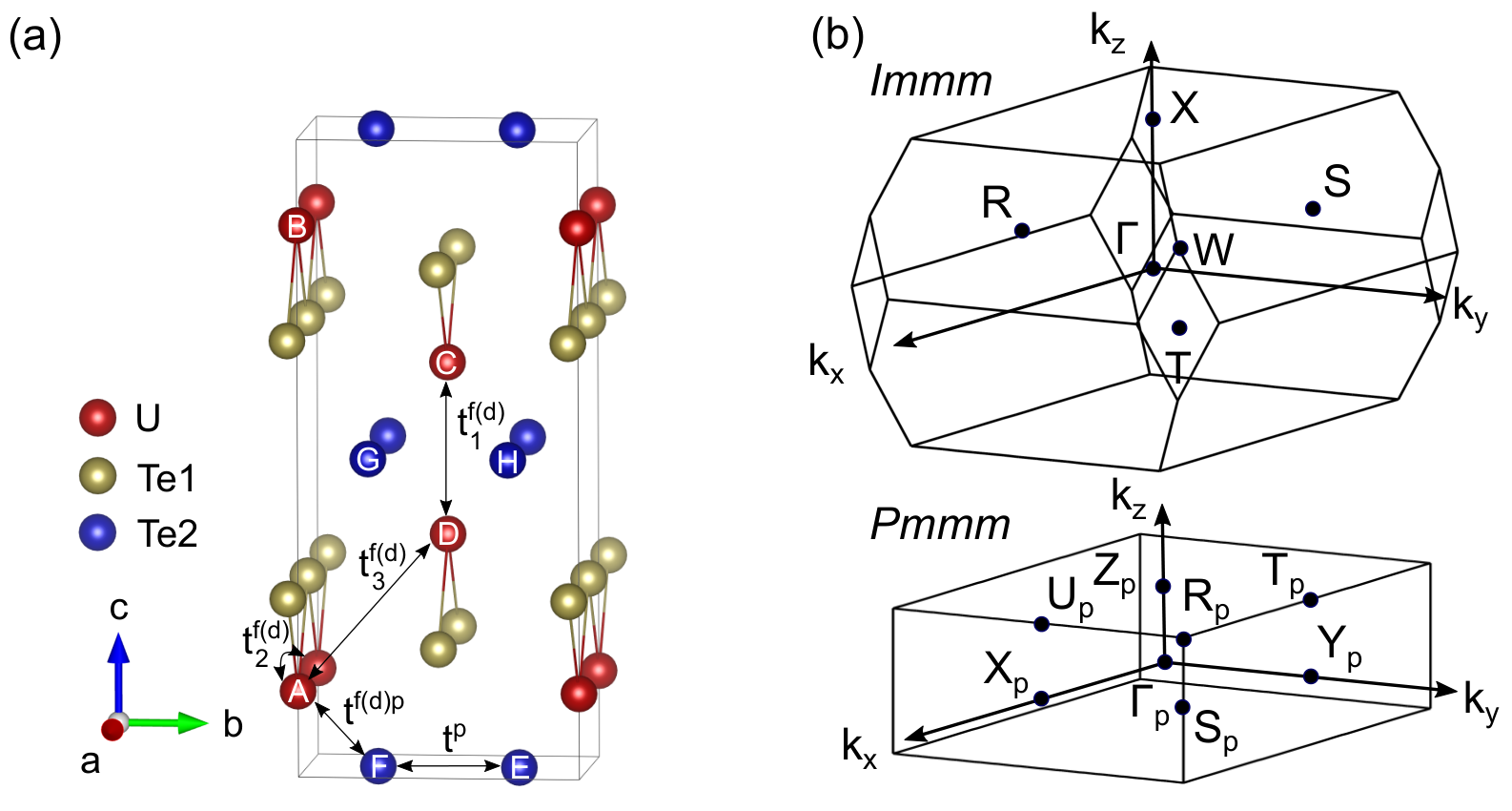
The DFT calculations clarified hole and electron FSs, indicating a rather simple electronic structure near the Fermi level Ishizuka et al. 2019; Xu et al. 2019. Therefore, we can construct a model including minimal hopping parameters [see Fig. 1(a)] which reproduces the low-energy electronic band structures in UTe2. We adopt an original unit cell of the space group to illustrate FSs (Fig. 2), while a primitive unit cell () with a folded Brillouin zone (BZ) [Fig. 1(b)] is adopted for convenience to calculate magnetic fluctuation and superconductivity. The resultant model is a - or -band periodic Anderson model, when we take into account on-site Coulomb interaction of -electrons. In addition, a sublattice-dependent antisymmetric spin-orbit coupling (sASOC) Sigrist et al. 2014; Maruyama et al. 2012; Fischer et al. 2011; Yanase 2016 is introduced in accordance with the local inversion symmetry breaking at uranium atoms. Since uranium atoms form a ladder structure with local site symmetry , a Rashba-type sASOC appears with opposite coupling constants . This sASOC induces magnetic anisotropy consistent with experiments Ran et al. 2019a; Aoki et al. 2019. Here and hereafter, we set sASOC as . Details of the tight-binding model are given in Appendix A. We study the pressure effect by introducing an enhancement factor of hopping integrals. Hopping integrals of -electrons and hybridization between and other orbitals are multiplied by , while at ambient pressure. To translate into a real pressure, DFT calculations for UTe2 under pressure are required. However, the lattice parameters under pressure have not been reported, and thus, we left it for a future study.
The band structure and FSs are shown in Figs. S1 and 2. The weight of Te2 -, U -, and U -electrons is illustrated by color. The band structure exhibits flat -electron bands and one-dimensional dispersive - and -electron bands, each of which contributes to the FSs. For a range of , the topology of FS is consistent with ARPES Miao et al. 2020 and DFT calculations with intermediate Ishizuka et al. 2019. Conducting directions of - and -electrons are orthogonal, and quasi-2D rectangular FSs are formed. Owing to the contribution of itinerant -electrons the hole FS is bent and encloses (-point) as shown in Figs. 2(b) and 2(d). For [Fig. 2(b)], a large -orbital component is found near the -point. When the factor is increased by pressure, the orbital character on FSs is largely changed, although FSs are only slightly changed. For [Fig. 2(d)] we see a sizable -electron component in a broad region on FSs. The change in orbital character results in a peculiar magnetic and superconducting phase diagram as we show below.

III Magnetic fluctuation
We apply the random phase approximation for the Coulomb interaction of -electrons. Diagonal magnetic susceptibilities, , , and , are calculated from the susceptibility matrix of -electrons (see Appendix B), and the momentum dependence is shown in Fig. 3. For , we see a ferromagnetic fluctuation with Ising anisotropy along the -axis [Figs. 3(a), 3(g), and 3(m)]; at maximum is much larger than and . This is in good agreement with experiments at ambient pressure Ran et al. 2019a; Aoki et al. 2019. On the other hand, with increasing , ferromagnetic fluctuation gradually changes to the antiferromagnetic fluctuation. This result implies that the magnetically ordered phase observed under pressure Braithwaite et al. 2019; Knebel et al. 2020; Aoki et al. 2020; Thomas et al. 2020 is an antiferromagnetic phase. The magnetic anisotropy at the ordering vector is reduced by pressure; for instance, at for .
Growth of antiferromagnetic fluctuation originates from the change in orbital characters. Although the FSs show nesting property irrespective of the factor , the -electron component is negligible on the nested part of FSs for . Therefore, -electrons around the -point enhance the ferromagnetic fluctuation rather than antiferromagnetic one. However, for the -electron component is sizable on the nested FSs, and therefore, antiferromagnetic fluctuation develops around a nesting vector . The -vector corresponds to antiparallel alignment of the magnetic moment along Uranium chains. As for an intra-unit-cell structure, parallel alignment of magnetic moment between sublattices is favored. This means that, from the view point of augmented cluster multipole Watanabe and Yanase 2017; Hayami et al. 2014, the obtained magnetic fluctuation is classified as even-parity magnetic dipole fluctuation, and the odd-parity magnetic fluctuation Ishizuka and Yanase 2018 is not pronounced in UTe2.

IV Superconductivity
Now, we clarify superconducting instability by solving the linearized Eliashberg equation (see Appendix C). In the point group symmetry, the order parameter of superconductivity is classified as one of the eight irreducible representations. In general, the Eliashberg equation is separable for each representation, and thus we obtain eight eigenvalues for each parameter set. Superconductivity occurs when the maximum eigenvalue is unity. Thus, we can determine what is the most stable superconducting state by comparing the eigenvalues.
The dependence of eigenvalues is shown in Fig. 4(a). We see that the pairing state is most stable at , indicating that the spin-triplet superconductivity is stabilized by the ferromagnetic fluctuation with Ising anisotropy. For and , another spin-triplet pairing state with symmetry is stabilized by incommensurate magnetic fluctuations. The and states are almost degenerate, and a more realistic model taking into account multiplet of -electrons should be analyzed to compare the two states. Both and states are monotonically suppressed by increasing , and finally the state becomes predominant. Thus, our results not only predict the odd-parity spin-triplet superconductivity of UTe2 at ambient pressure but also indicate the spin-singlet superconductivity under pressure. The latter is natural since the antiferromagnetic fluctuation usually stabilizes a -wave or -wave superconductivity, as widely believed for cuprates Yanase et al. 2003 and iron-based superconductors Hosono and Kuroki 2015.
We also evaluate the critical temperature of superconducting instability based on the criterion and show the results in Fig. 4(b). The , , and states may be stabilized below . The pairing symmetry for each is consistent with Fig. 4(a). The transition temperature is highest at , in contrast to the experiment. We need further study for quantifying the transition temperature and the pressure dependence, for instance, by conducting DFT calculations under pressure.
To clarify the , , and states, we here discuss the order parameter of superconductivity. In a standard manner, it is described as , with the Pauli matrix for spin degree of freedom. Although we omitted indices of sublattices for simplicity, intrasublattice and intersublattice components have similar structures (see Appendix C). Thus, we show the maximum magnitude of intrasublattice components in whole momentum space (Table 1). To be precise, all the states possess mixed spin-singlet and spin-triplet components since a sublattice-dependent parity mixing generally occurs in locally noncentrosymmetric systems Maruyama et al. 2012; Fischer et al. 2011. What kind of the parity mixing occurs is understood from the compatibility relation, and the basis functions are given in Table 2. According to Tables 1 and 2, the predominant component for the state is , while for the state it is . Because these states are almost degenerate, the -vector can rotate in the crystallographic - plane. Thus, the Knight shift would be almost unchanged irrespective of the field direction, consistent with experimental results Nakamine et al. 2019; Ishida. For the state, a spin-singlet -wave component with sign change, , is predominant. The subdominant spin-triplet component, , is considerably small.
Transforming to the band basis, we obtain superconducting gap structures illustrated in Fig. 5. As we considered the Coulomb interaction of -electrons for superconductivity, the gap amplitudes are large on a part of FSs having a sizable contribution from -electrons. Therefore, the gap structure is highly anisotropic in all the superconducting states. In accordance with group theories Ishizuka et al. 2019; Yarzhemsky and Teplyakov 2020, we see symmetry-protected point nodes along the axis in the state, while the line node is absent in agreement with Blount’s theorem. However, the gap minima, where the gap amplitude is not exactly zero, appears as a pseudoline node on the plane [Fig. 5(b)] because . Similarly, the state shows a pseudo line node on , while it is a full-gap state in an exact sense. It needs further investigations for the pseudo line node in comparison with experiments proposing point nodal gap Ran et al. 2019a; Metz et al. 2019 because the gap structure is significantly band dependent.

V Multiple superconducting phases
Based on the superconducting instability evaluated in Fig. 4(b), we illustrate our interpretation of the experimentally observed multiple superconducting phases in UTe2 Braithwaite et al. 2019; Ran et al. 2020; Lin et al. 2020; Knebel et al. 2020; Aoki et al. 2020; Thomas et al. 2020. In Fig. 6(a), we draw a superconducting phase transition from the odd-parity or state to the even-parity state under the applied pressure, coinciding with crossover in magnetic fluctuations from ferromagnetic to antiferromagnetic. When the transition temperatures of the two states are close to each other, the coexistent phase is naturally expected, that is, either the or state with mixed even-/odd-parity, and the space inversion symmetry is spontaneously broken. The time-reversal symmetry is preserved in the former, while the latter is symmetric.
We also propose superconducting phases in the magnetic field under pressure [Fig. 6(b)]. In this magnetic field, and representations are reduced to the same representation, and therefore, the state is possible. This state almost avoids the paramagnetic depairing effect because the equal spin pairing along the -axis is dominant. Thus, the upper critical field is naturally higher than that of the spin-singlet state, and the superconducting phase diagram with a tricritical point is expected. Indeed, multiple superconducting phases as in Fig. 6(b) have been reported in recent experiments Knebel et al. 2020; Aoki et al. 2020.
VI Conclusion
In this paper, we constructed a -band periodic Anderson model as a reasonably realistic and easy-handled model for UTe2. The model reveals not only the ferromagnetic fluctuation with the easy -axis at ambient pressure but also the antiferromagnetic fluctuation under pressures. Accordingly, spin-triplet superconductivity of either or representation is stabilized by the ferromagnetic fluctuation, while spin-singlet superconductivity of representation is favored by the antiferromagnetic fluctuation.
These results enable us to draw phase diagrams in reasonable agreement with experiments. As a consequence, a mixed even-/odd-parity superconducting state with spontaneous inversion symmetry breaking is predicted. Such a phase was referred to in a review article Leggett 1975 forty years ago published with the comment ”there seems at present no experimental evidence.” Even at present, spontaneous ordering of mixed even-/odd-parity superconductivity has not been reported. UTe2 may be the first material. Exploration of exotic superconducting properties will be the next issue.
Acknowledgements.
We appreciate helpful discussions with S. Kanasugi, K. Ishida, K. Izawa, S. Fujimori, D. Aoki, T. Shibauchi, A. H. Nevidomskyy, J. Flouquet, J.-P. Brison, and G. Knebel. This work was supported by JSPS KAKENHI (Grants No. JP18H04225, No. JP18H05227, No. JP18H01178, and No. 20H05159).Appendix A Tight-binding model
A periodic Anderson model is given by , where is the tight-binding model for a noninteracting part and represents the on-site Coulomb interaction of -electrons. Here, we introduce details of the tight-binding model for UTe2,
| (1) |
which contains a kinetic energy term and sublattice-dependent antisymmetric spin-orbit coupling (sASOC) term .
The Hamiltonian of the kinetic energy term is given by
| (2) |
where
| (3) |
| (4) |
| (5) |
and
| (6) |
with the primitive unit cell . The annihilation (creation) operators of U , U , and Te2 electrons with pseudospin on a sublattice and are represented by , , and , respectively. The single-electron kinetic energy is described by taking into account the hopping integrals up to the third order shown in Fig. 1 of the main text,
| (7) | ||||
| (8) | ||||
| (9) | ||||
| (10) |
| (11) | ||||
| (12) | ||||
| (13) | ||||
| (14) | ||||
| (15) | ||||
| (16) | ||||
| (17) | ||||
| (18) |
The tight-binding parameters in Table 3 reproduce the Fermi surfaces (FSs) observed in an ARPES experiment Miao et al. 2020 and DFT calculations Ishizuka et al. 2019. As shown in the main text, the model for this parameter set shows enhanced ferromagnetic fluctuation with the easy -axis in agreement with experiments at ambient pressure Ran et al. 2019a; Aoki et al. 2019. To investigate effects of pressure, we introduce an enhancement factor for the hopping integrals concerned with the electrons. The corresponding tight-binding parameters are multiplied by with , while at ambient pressure.
The sASOC term is written as
| (19) |
where , , and are the Pauli matrices representing the spin, intra-ladder sublattice, and inter-ladder sublattice degrees of freedom, respectively. We set for simplicity.
In Fig. 7 we compare the band structure obtained from the tight-binding Hamiltonian Eq. (1) with that from a DFT calculation with an intermediate Coulomb interaction eV. Although the number of bands is different because we neglect orbital degeneracy in the tight-binding model, flat U 5 band and dispersive U 6 and Te 5 bands are reasonably described. In particular, the low-energy band structure is appropriately reproduced. The FSs (see Fig. 2 in the main text and Fig. 8) as well as the weight of U 5, U 6 and Te 5 electrons on the FSs are similar between the tight-binding model and the DFT+ calculation.
| Onsite | ||||||||||||
| Nearest | ||||||||||||
| 2nd Nearest | ||||||||||||
| 3rd Nearest | ||||||||||||


Appendix B Magnetic Susceptibility
The susceptibility matrix in the -orbital subspace is calculated by the random phase approximation (RPA) as
| (20) |
where the irreducible susceptibility is defined as . and are the -orbital Green’s function and the bare irreducible vertex, respectively. Here we introduce site-resolved magnetic susceptibilities
| (21) |
for . We calculate the magnetic susceptibility on Uranium atoms by
| (22) |
where represents the number of Uranium atoms. Figure 9 shows the dependence of the magnetic susceptibility. The magnetic susceptibility and its anisotropy grow with because the susceptibility is divergent at the magnetic critical point. The larger (lower ) enhances the anisotropy leading to the spin-triplet and superconductivity.
Appendix C Eliashberg equation and gap function
Superconductivity is investigated by solving the linearized Eliashberg equation formulated as
| (23) |
with . The effective pairing interaction is described by the RPA susceptibility as
| (24) |
Solving the Eliashberg equation, we obtain an eigenvalue and a gap function for each irreducible representation. Eigenvalues at a fixed temperature are shown in Fig. 4(a) in the main text, where the Coulomb interaction is set as Table 4 so that sizable eigenvalues are obtained. A similar result is obtained for a fixed . We actually show the -dependence of transition temperatures for a fixed in Fig. 4(b). The maximum magnitudes of each spin component in the intrasublattice gap function are shown in the main text (Table 1), while those of the intersublattice gap function are shown in Table 5.
References
- Ran et al. (2019a) S. Ran, C. Eckberg, Q.-P. Ding, Y. Furukawa, T. Metz, S. R. Saha, I.-L. Liu, M. Zic, H. Kim, J. Paglione, and N. P. Butch, Science 365, 684 (2019a).
- Qi and Zhang (2011) X.-L. Qi and S.-C. Zhang, Rev. Mod. Phys. 83, 1057 (2011).
- Sato and Fujimoto (2016) M. Sato and S. Fujimoto, J. Phys. Soc. Jpn. 85, 072001 (2016).
- Sato and Ando (2017) M. Sato and Y. Ando, Rep. Prog. Phys. 80, 076501 (2017).
- Aoki et al. (2019) D. Aoki, A. Nakamura, F. Honda, D. Li, Y. Homma, Y. Shimizu, Y. J. Sato, G. Knebel, J.-P. Brison, A. Pourret, D. Braithwaite, G. Lapertot, Q. Niu, M. Vališka, H. Harima, and J. Flouquet, J. Phys. Soc. Jpn. 88, 043702 (2019).
- Tokunaga et al. (2019) Y. Tokunaga, H. Sakai, S. Kambe, T. Hattori, N. Higa, G. Nakamine, S. Kitagawa, K. Ishida, A. Nakamura, Y. Shimizu, Y. Homma, D. Li, F. Honda, and D. Aoki, J. Phys. Soc. Jpn. 88, 073701 (2019).
- Sundar et al. (2019) S. Sundar, S. Gheidi, K. Akintola, A. M. Côté, S. R. Dunsiger, S. Ran, N. P. Butch, S. R. Saha, J. Paglione, and J. E. Sonier, Phys. Rev. B 100, 140502(R) (2019).
- Knebel et al. (2019) G. Knebel, W. Knafo, A. Pourret, Q. Niu, M. Vališka, D. Braithwaite, G. Lapertot, M. Nardone, A. Zitouni, S. Mishra, I. Sheikin, G. Seyfarth, J.-P. Brison, D. Aoki, and J. Flouquet, J. Phys. Soc. Jpn. 88, 063707 (2019).
- Knafo et al. (2019) W. Knafo, M. Vališka, D. Braithwaite, G. Lapertot, G. Knebel, A. Pourret, J.-P. Brison, J. Flouquet, and D. Aoki, J. Phys. Soc. Jpn. 88, 063705 (2019).
- Miyake et al. (2019) A. Miyake, Y. Shimizu, Y. J. Sato, D. Li, A. Nakamura, Y. Homma, F. Honda, J. Flouquet, M. Tokunaga, and D. Aoki, J. Phys. Soc. Jpn. 88, 063706 (2019).
- Imajo et al. (2019) S. Imajo, Y. Kohama, A. Miyake, C. Dong, M. Tokunaga, J. Flouquet, K. Kindo, and D. Aoki, J. Phys. Soc. Jpn. 88, 083705 (2019).
- Mineev (2020) V. P. Mineev, JETP Letters (2020), 10.1134/S0021364020120036.
- Nakamine et al. (2019) G. Nakamine, S. Kitagawa, K. Ishida, Y. Tokunaga, H. Sakai, S. Kambe, A. Nakamura, Y. Shimizu, Y. Homma, D. Li, F. Honda, and D. Aoki, J. Phys. Soc. Jpn. 88, 113703 (2019).
- Jiao et al. (2020) L. Jiao, S. Howard, S. Ran, Z. Wang, J. O. Rodriguez, M. Sigrist, Z. Wang, N. P. Butch, and V. Madhavan, Nature 579, 523 (2020).
- Bae et al. (2019) S. Bae, H. Kim, S. Ran, Y. S. Eo, I.-L. Liu, W. Fuhrman, J. Paglione, N. P. Butch, and S. Anlage, arXiv e-prints , arXiv:1909.09032 (2019), arXiv:1909.09032 [cond-mat.supr-con] .
- Kittaka et al. (2020) S. Kittaka, Y. Shimizu, T. Sakakibara, A. Nakamura, D. Li, Y. Homma, F. Honda, D. Aoki, and K. Machida, Phys. Rev. Research 2, 032014 (2020).
- Metz et al. (2019) T. Metz, S. Bae, S. Ran, I.-L. Liu, Y. S. Eo, W. T. Fuhrman, D. F. Agterberg, S. M. Anlage, N. P. Butch, and J. Paglione, Phys. Rev. B 100, 220504(R) (2019).
- (18) K. Izawa and S. Hosoi, private communication .
- Hayes et al. (2020) I. M. Hayes, D. S. Wei, T. Metz, J. Zhang, Y. S. Eo, S. Ran, S. R. Saha, J. Collini, N. P. Butch, D. F. Agterberg, A. Kapitulnik, and J. Paglione, arXiv e-prints , arXiv:2002.02539 (2020), arXiv:2002.02539 [cond-mat.str-el] .
- Braithwaite et al. (2019) D. Braithwaite, M. Vališka, G. Knebel, G. Lapertot, J.-P. Brison, A. Pourret, M. E. Zhitomirsky, J. Flouquet, F. Honda, and D. Aoki, Communications Physics 2, 147 (2019).
- Ran et al. (2020) S. Ran, H. Kim, I.-L. Liu, S. R. Saha, I. Hayes, T. Metz, Y. S. Eo, J. Paglione, and N. P. Butch, Phys. Rev. B 101, 140503(R) (2020).
- Lin et al. (2020) W.-C. Lin, D. J. Campbell, S. Ran, I.-L. Liu, H. Kim, A. H. Nevidomskyy, D. Graf, N. P. Butch, and J. Paglione, npj Quantum Materials 5, 68 (2020).
- Knebel et al. (2020) G. Knebel, M. Kimata, M. Vališka, F. Honda, D. Li, D. Braithwaite, G. Lapertot, W. Knafo, A. Pourret, Y. J. Sato, Y. Shimizu, T. Kihara, J.-P. Brison, J. Flouquet, and D. Aoki, J. Phys. Soc. Jpn. 89, 053707 (2020).
- Aoki et al. (2020) D. Aoki, F. Honda, G. Knebel, D. Braithwaite, A. Nakamura, D. Li, Y. Homma, Y. Shimizu, Y. J. Sato, J.-P. Brison, and J. Flouquet, J. Phys. Soc. Jpn. 89, 053705 (2020).
- Thomas et al. (2020) S. M. Thomas, F. B. Santos, M. H. Christensen, T. Asaba, F. Ronning, J. D. Thompson, E. D. Bauer, R. M. Fernandes, G. Fabbris, and P. F. S. Rosa, Science Advances 6 (2020), 10.1126/sciadv.abc8709.
- Ran et al. (2019b) S. Ran, I.-L. Liu, Y. S. Eo, D. J. Campbell, P. M. Neves, W. T. Fuhrman, S. R. Saha, C. Eckberg, H. Kim, D. Graf, F. Balakirev, J. Singleton, J. Paglione, and N. P. Butch, Nat. Phys. 15, 1250 (2019b).
- Ishizuka et al. (2019) J. Ishizuka, S. Sumita, A. Daido, and Y. Yanase, Phys. Rev. Lett. 123, 217001 (2019).
- Leggett (1975) A. J. Leggett, Rev. Mod. Phys. 47, 331 (1975).
- Sauls (1994) J. Sauls, Advances in Physics 43, 113 (1994).
- Joynt and Taillefer (2002) R. Joynt and L. Taillefer, Rev. Mod. Phys. 74, 235 (2002).
- Sigrist and Ueda (1991) M. Sigrist and K. Ueda, Rev. Mod. Phys. 63, 239 (1991).
- Nevidomskyy (2020) A. H. Nevidomskyy, arXiv e-prints , arXiv:2001.02699 (2020), arXiv:2001.02699 [cond-mat.supr-con] .
- Machida (2020) K. Machida, J. Phys. Soc. Jpn. 89, 033702 (2020).
- Yanase and Shiozaki (2017) Y. Yanase and K. Shiozaki, Phys. Rev. B 95, 224514 (2017).
- Daido et al. (2019) A. Daido, T. Yoshida, and Y. Yanase, Phys. Rev. Lett. 122, 227001 (2019).
- Ono et al. (2019) S. Ono, Y. Yanase, and H. Watanabe, Phys. Rev. Research 1, 013012 (2019).
- Skurativska et al. (2020) A. Skurativska, T. Neupert, and M. H. Fischer, Phys. Rev. Research 2, 013064 (2020).
- Ono et al. (2020) S. Ono, H. C. Po, and H. Watanabe, Science Advances 6 (2020), 10.1126/sciadv.aaz8367.
- Shick and Pickett (2019) A. B. Shick and W. E. Pickett, Phys. Rev. B 100, 134502 (2019).
- Xu et al. (2019) Y. Xu, Y. Sheng, and Y.-f. Yang, Phys. Rev. Lett. 123, 217002 (2019).
- Miao et al. (2020) L. Miao, S. Liu, Y. Xu, E. C. Kotta, C.-J. Kang, S. Ran, J. Paglione, G. Kotliar, N. P. Butch, J. D. Denlinger, and L. A. Wray, Phys. Rev. Lett. 124, 076401 (2020).
- Harima (2020) H. Harima, JPS Conf. Proc. 29, 011006 (2020).
- Fujimori et al. (2019) S.-i. Fujimori, I. Kawasaki, Y. Takeda, H. Yamagami, A. Nakamura, Y. Homma, and D. Aoki, J. Phys. Soc. Jpn. 88, 103701 (2019).
- Niu et al. (2020) Q. Niu, G. Knebel, D. Braithwaite, D. Aoki, G. Lapertot, G. Seyfarth, J.-P. Brison, J. Flouquet, and A. Pourret, Phys. Rev. Lett. 124, 086601 (2020).
- Sigrist et al. (2014) M. Sigrist, D. F. Agterberg, M. H. Fischer, J. Goryo, F. Loder, S.-H. Rhim, D. Maruyama, Y. Yanase, T. Yoshida, and S. J. Youn, J. Phys. Soc. Jpn. 83, 061014 (2014).
- Maruyama et al. (2012) D. Maruyama, M. Sigrist, and Y. Yanase, J. Phys. Soc. Jpn. 81, 034702 (2012).
- Fischer et al. (2011) M. H. Fischer, F. Loder, and M. Sigrist, Phys. Rev. B 84, 184533 (2011).
- Yanase (2016) Y. Yanase, Phys. Rev. B 94, 174502 (2016).
- Watanabe and Yanase (2017) H. Watanabe and Y. Yanase, Phys. Rev. B 96, 064432 (2017).
- Hayami et al. (2014) S. Hayami, H. Kusunose, and Y. Motome, Phys. Rev. B 90, 024432 (2014).
- Ishizuka and Yanase (2018) J. Ishizuka and Y. Yanase, Phys. Rev. B 98, 224510 (2018).
- Yanase et al. (2003) Y. Yanase, T. Jujo, T. Nomura, H. Ikeda, T. Hotta, and K. Yamada, Phys. Rep. 387, 1 (2003).
- Hosono and Kuroki (2015) H. Hosono and K. Kuroki, Physica C: Superconductivity and its Applications 514, 399 (2015).
- (54) See Supplemental Material for details.
- (55) K. Ishida, private communication .
- Yarzhemsky and Teplyakov (2020) V. Yarzhemsky and E. Teplyakov, Phys. Lett. A 384, 126724 (2020).