A Search for Axionic Dark Matter Using the Magnetar PSR J17452900
Abstract
We report on a search for dark matter axion conversion photons from the magnetosphere of the Galactic Center magnetar PSR J17452900 using spectra obtained from the Karl G. Jansky Very Large Array.11 1 The National Radio Astronomy Observatory is a facility of the National Science Foundation operated under cooperative agreement by Associated Universities, Inc. No significant spectral features are detected. Using a hybrid model for PSR J17452900 and canonical assumptions about the dark matter density profile, we exclude axion models with axion-photon coupling –34 GeV-1 with 95% confidence over the mass ranges 4.2–8.4, 18.6–26.9, 33.0–41.4, 53.7–62.1, and 126.0–159.3 eV. If there is a dark matter cusp, the limits reduce to – GeV-1, which overlap some axion models for the observed mass ranges eV. These limits may be improved by modeling the stimulated emission that can boost the axion-photon conversion process.
I Introduction
The axion is a spin zero chargeless massive particle introduced to address the strong (charge-parity) problem in quantum chromodynamics (QCD; Peccei and Quinn 1977; Weinberg 1978; Wilczek 1978). If they exist, QCD axions are likely to be produced in the early universe, are a promising cold dark matter candidate Preskill et al. 1983; Dine and Fischler 1983; Abbott and Sikivie 1983, and may explain the cosmic matter-antimatter asymmetry Co and Harigaya 2019.
Axions couple to QCD and electromagnetism. The electromagnetic coupling suggests that axion-photon conversion can occur in the presence of magnetic fields, but the axion-photon coupling is weak ( GeV-1 for axion mass eV) Kim 1979; Shifman et al. 1980; Dine et al. 1981; Zhitnitskij 1980; Sikivie 1983. The relationship between and is linear, but the mass is not constrained; axion searches must span decades in .
Recent axion searches include CAST, which searched for Solar axions Arik and et al. CAST; Arik and et al. CAST, and haloscopes such as ADMX and HAYSTAC that use narrow-band resonant cavities to detect dark matter axions Asztalos and et al. ADMX; Asztalos and et al. 2010; Brubaker and et al. 2017; Zhong et al. 2018. There are also natural settings where telescopes may conduct sensitive and wide-band QCD axion searches Arvanitaki et al. 2015; Hook et al. 2018a; Huang et al. 2018; Mukherjee et al. 2018; Day and McDonald 2019; Battye et al. 2020; Leroy et al. 2020; Edwards et al. 2020; Mukherjee et al. 2020.
The Galactic Center magnetar PSR J17452900 offers an ideal setting for an axion conversion line search: it has a strong magnetic field ( G) Mori and et al. 2013 and should see the highest possible dark matter flux Hook et al. 2018a. Axions will encounter a plasma frequency at some radius that equals its mass, and the axion can resonantly convert into a photon at that location Hook et al. 2018a. The most promising axion mass range, 1–100 eV, corresponds to radio frequencies 200 MHz to 20 GHz.
In this Letter, we present broad-band radio telescope observations of PSR J17452900. We obtain 95% confidence limits on resonant axion-photon conversion emission line flux density from the magnetar spanning 40% of the 1–38.5 GHz band. We translate these flux limits into limits on versus based on a hybrid neutron star magnetosphere model and two limiting-case Galactic dark matter profiles. Finally, we discuss model caveats, limitations of the observations, and future observational and theoretical work to expand the vs. space probed by this technique.
| Band | Frequency | Program | Channel Width | Median | Integration | Median Beam | PA | MJD22 2 Modified Julian Date | rms33 3 The rms noise in spectra Gaussian-smoothed to channels of width (Column 5 and Equation 2). | |
|---|---|---|---|---|---|---|---|---|---|---|
| Obs. | Smoothed | Velocity | ||||||||
| (GHz) | (MHz) | (MHz) | (km s-1) | (s) | (arcsec) | (∘) | (mJy) | |||
| L | 1.008–2.032 | 14A-231 | 1 | 10 | 2000 | 10591 | 44 4 The quoted L-band beam is the continuum beam; the synthesized beam in the spectral cube is highly variable due to RFI and the large fractional bandwidth. | 1 | 56749 | 0.3355 5 The rms noise includes residual unmitigated RFI. |
| C | 4.487–6.511 | 14A-231 | 2 | 14 | 763 | 10591 | 3 | 56749 | 0.099 | |
| X | 7.987–10.011 | 14A-231 | 2 | 18 | 600 | 19148 | 1 | 56718 | 0.02666 6 The rms noise omits the central RFI feature and band edges. | |
| Ku | 12.988–15.012 | 14A-231 | 2 | 20 | 428 | 16156 | 1 | 56726 | 0.027 | |
| Ka | 30.476–32.524 | 14A-232 | 2 | 26 | 247 | 17053 | 3 | 56725 | 0.100 | |
| Ka | 32.476–34.524 | 14A-232 | 2 | 26 | 233 | 17053 | 3 | 56725 | 0.116 | |
| Ka | 34.476–36.524 | 14A-232 | 2 | 28 | 236 | 17053 | 4 | 56725 | 0.165 | |
| Ka | 36.476–38.524 | 14A-232 | 2 | 28 | 224 | 17053 | 3 | 56725 | 0.152 | |
II Observations
Interferometric observations of Sgr A* were obtained from the National Science Foundation’s Karl G. Jansky Very Large Array (VLA 77 7 The National Radio Astronomy Observatory is a facility of the National Science Foundation operated under cooperative agreement by Associated Universities, Inc.) data archive. We selected sessions: (1) to maximize on-target integration time, (2) with adequate angular resolution to separate PSR J17452900 from Sgr A* (1.7” in both coordinates), (3) to maximize total bandwidth, and (4) to adequately sample the expected emission line bandwidth. VLA A-configuration observations of Sgr A*, 14A-231 and 14A-232, meet these criteria, spanning 40% of the 1–38.5 GHz range (Table 1). The gaps in this range are not covered by any extant observations that meet the above criteria.
Each session used the flux density calibrator J1331+3030 (3C286) and the bandpass calibrator J17331304. For L- and C-band, the bandpass calibrator was also used for complex gain calibration. The other bands used J17443116 for complex gain calibration. Observations of the gain calibrator were interleaved with Sgr A* integrations with 8–30 min cadence. Each band was observed for a full transit of Sgr A*. The correlator was configured to obtain four polarization products (only the two parallel-hand products were used to form Stokes-I spectra below), in 8 to 64 adjacent 64-channel spectral windows with 128 MHz bandwidth each. The spectral windows were divided into 2 or 4 slightly overlapping baseband groups. The L-band configuration differed: it used spectral windows of 64 MHz bandwith and 1 MHz channels. All sampling was 8-bit except for the Ka-band session, which used 3-bit sampling. Correlator dump times were 1–5 s.
III Data Reduction
All data reduction tasks were performed using CASA 88 8 McMullin, J. P., Waters, B., Schiebel, D., Young, W., & Golap, K. 2007, Astronomical Data Analysis Software and Systems XVI (ASP Conf. Ser. 376), ed. R. A. Shaw, F. Hill, & D. J. Bell (San Francisco, CA: ASP), 127. See also https://science.nrao.edu/facilities/vla/data-processing/pipeline for the CASA calibration pipeline and https://science.nrao.edu/facilities/vla/data-processing for VLA calibration and analysis.. After data flagging, we applied the flux, delay, atmospheric transmission, complex bandpass, and complex gain calibration to the target field. We then performed in-beam phase self-calibration using the Sgr A* continuum, which ranged from 0.5 to 5.6 Jy (L- to Ka-band). We imaged the continuum field and identified the continuum emission of PSR J17452900 (20–5 mJy in L to Ka bands) to confirm its coordinate offset from Sgr A*.
We fit a 2D Gaussian to the Sgr A* continuum to set the origin for relative astrometry to locate PSR J17452900 based on the bootstrap proper motion solution obtained by Bower et al. 2015 that assumes no acceleration or core shift. At the observed angular resolution, Sgr A* is consistent with being a point source. Coordinate offsets from Sgr A* were arcsec in all epochs; offsets between epochs differed by no more than 1 mas. The predicted offsets of PSR J17452900 from Sgr A* are consistent with the observed continuum position of the magnetar.
We fit and subtracted a linear continuum spectrum from the data in UV (image Fourier) space and formed spectral image cubes using pixels that over-sampled the synthesized beams (which vary across each cube). Sgr A* shows narrow-band spectral structure after the continuum subtraction, some of which are attributable to known molecular lines such as the 14.4881 GHz H2CO and 36.795 GHz CH3CN. Sidelobes from these features are cleaned during cube deconvolution and do not significantly contaminate the magnetar spectrum. The zero-mean magnetar spectra typically reach the theoretical noise.
At the position of the magnetar, we extract a spectrum by summing pixels over the (frequency-dependent) synthesized 2D Gaussian beam. We correct the spectrum for the beam size to capture the total flux density of a point source separately for every channel. In order to assess the significance of features in the magnetar spectrum, which can be highly variable channel-to-channel due to radio frequency interference (RFI) or band edges, we create a noise spectrum by measuring the off-source rms sky noise in each channel. This allows us to create a significance spectrum for each band. We scale the noise spectrum to match the spectral noise measured toward PSR J17452900 (this correction is typically a few percent).
The fractional bandwidth predictions for the expected signal range from Hook et al. 2018a, where is the axion velocity dispersion, to Huang et al. 2018. We adopt the spinning mirror model whereby the Doppler broadening is dominated by the neutron star rotation Battye et al. 2020, producing, on average, , where is the neutron star’s angular frequency, is the eccentricity of the elliptical critical surface (which we and Battye et al. 2020 set to unity), and is the axion-photon conversion radius. For the latter, we adopt the formulation of Hook et al. 2018a, assuming polar orientation angle and magnetic offset axis (see below, where we marginalize over these unknown angles; as Leroy et al. 2020 show, ray-tracing is the technically correct approach, and tends to show less variation with these angles than the analytic treatment):
| (1) |
where is the neutron star radius, is the magnetic field, and 4.1 eV corresponds to an observed frequency of 1 GHz. This leads to an expected line bandwidth:
| (2) |
The spin period of PSR J17452900 is 3.76 s Kennea and et al. 2013 and the magnetic field is G Mori and et al. 2013. The expected line width is therefore .
The VLA correlator spectral windows have a strong response dropoff on edge channels and on the edges of the basebands. These channels lack the signal-to-noise for calibration and are flagged, which typically creates single-channel gaps in the spectrum and decreased sensitivity on the spectrum edges. The flagged channels are much narrower than the expected line width. We smooth the magnetar and noise spectra to the expected line width (Equation 2) using a Gaussian kernel Price-Whelan et al. 2018, and interpolate across missing channels during smoothing (the resulting statistics are not substantially altered by this loss of strict channel-to-channel independence). In L-band there are gaps in the spectrum where RFI-flagged spectral regions are wider than the smoothing kernel.
Table 1 lists synthesized beam parameters, channel widths, and spectral rms noise values. The Supplemental Material 99 9 See Supplemental Material at [URL]. presents the magnetar flux, noise, and signal-to-noise spectra.

IV Results
We detect no significant single-channel emission features in the observed bands. The only two channels above in emission were found in Ka-band (3.1 and 3.5). These departures are consistent with Gaussian noise statistics.
After establishing the lack of significant detections in the observed spectra, we form 95% confidence limits from the sky noise spectra. Figure 1 presents these single-channel confidence limits. These are model-independent limits on the flux density of photons produced by axion conversion in the magnetosphere of PSR J17452900 1010 10 Our assumption about the expected signal bandwidth does depend on models for the magnetar, but is .. We present these limits to enable models not treated below to be translated into axion limits.
V Analysis
Limits on the axion-photon coupling obtained from observed flux density limits depend on the magnetar magnetospheric and axion-photon conversion model and on the behavior of the dark matter at the Galactic Center. Our choices — as well as alternatives — are discussed below.
V.1 The Magnetar Model
Hook et al. Hook et al. 2018a predict the photon flux from axion conversion in a neutron star magnetosphere using a variant of the Goldreich and Julian Goldreich and Julian 1969 model. The observed flux density depends on the local dark matter density () and its velocity dispersion () and on the neutron star mass, radius, magnetic field, rotation period, distance, viewing angle with respect to the rotation axis, and magnetic misalignment angle from the spin axis (, , , , , , and , respectively). It also depends on and . Equations 11–13 in Hook et al. 2018a, modified for the expected bandwidth (Equation 2), yield an expression for the emission line flux density normalized to fiducial values for a nearby pulsar:
| (3) |
where . The axion velocity at the conversion point (see Supplement) is included to correct the conversion probability presented in Hook et al. 2018a, as discussed in Leroy et al. 2020. For a given line sensitivity (or observed flux density limit spectrum), one can obtain a track in versus space above which is excluded at some confidence level.
For PSR J17452900, we assume a radius km and mass M⊙. Using the Navarro-Frenk-White (NFW Navarro et al. 1996) Galactic dark matter profile model of McMillan 2017, which has Galactic Center distance kpc (in agreement with the S2 stellar orbital measurement around Sgr A* Abuter et al. 2019), scale radius kpc, and local dark matter energy density GeV cm-3 (see below), one obtains an axion mass-dependent expression for :
| (4) |
The angular term in Equation V.1 relies on the unknown viewing and magnetic field misalignment angles, so we marginalize over all possible orientations while keeping track of the fraction of the magnetar spin period (if any) that has (see Supplement). If the conversion radius is less than the neutron star radius, then no conversion occurs and the photon flux vanishes Hook et al. 2018a. The analytic value of is a conservative estimate; ray-tracing suggests that the actual axion-photon conversion can occur over a larger range of angles Leroy et al. 2020. Contrary to Hook et al. 2018a, we find that conversion can still occur up to and beyond 10 GHz. At the low end of the observed Ka-band range, 2.1% of all possible have at all times; at the high end of the band, this increases to 5.6%. At the high end of the observed Ku band, the fraction of orientations with no emission decreases to 0.16%.
V.2 Axion Constraints from Dark Matter Models
Following Hook et al. 2018a, we use two dark matter models — a generic NFW model and the NFW model plus a central dark matter spike — that roughly bound the weakest and strongest constraints on given the magnetar model unless the Galactic Center dark matter is cored (see below and Discussion). We use the NFW dark matter model from McMillan 2017 with , kpc, kpc, km s-1, and GeV cm-3, which predicts a dark matter density of GeV cm-3 at the 0.1 pc radial distance of the magnetar. The assumed physical distance of PSR J17452900 from Sgr A* — itself assumed to reside at the center of the dark matter distribution — is the projected distance (absent an acceleration measurement, one cannot determine the physical distance between Sgr A* and the magnetar Bower et al. 2015, but if the magnetar is gravitationally bound to Sgr A*, then the projected separation is likely to be a good approximation for the physical separation). For the dark matter spike, we use the above NFW profile modified to include a spike radial index and extent kpc, which corresponds to a 99.7% upper limit on deviations from a black hole-only orbit of the S2 star about Sgr A* Lacroix 2018. This model predicts a dark matter density of GeV cm-3 at the magnetar position. All else equal, this dark matter spike model can be considered to be a best-case constraint on . The two models span a factor of in dark matter density, which is a factor of 100 in the constraint. Future studies of the dynamics in the central parsec should improve constraints on the dark matter density encountered by PSR J17452900.
Table 2 lists the median 95% confidence limits on obtained from these end-case dark matter models for each observed band. Figure 2 shows the limits for the two models versus frequency and axion mass. The limits obtained for the standard NFW profile reach GeV-1, which is a factor of 40 above the strongest-coupling theoretical model Di Luzio et al. 2017. The limits obtained for the dark matter spike model impinge on the family of theoretical models Di Luzio et al. 2017 for in 33.0–41.4 eV, 53.7–62.1 eV, and 126.0–159.3 eV, but do not exclude the canonical KSVZ or DFSZ models Kim 1979; Shifman et al. 1980; Dine et al. 1981; Zhitnitskij 1980. If the Galactic dark matter has a flat profile inward of 0.5 kpc (i.e. it is “cored”), then the predicted dark matter density is 12 GeV cm-3 at the magnetar, the limits on are a factor of 100 above the NFW profile limits, and the limits are less constraining than the CAST limits.

| Axion Mass | Median 95% Confidence Limits | |
|---|---|---|
| (eV) | NFW Profile | DM Spike |
| (GeV-1) | (GeV-1) | |
| 4.2--8.41111 11 There are gaps in the coverage of this mass range (see Figure 2). | ||
| 18.6–26.9 | ||
| 33.0–41.4 | ||
| 53.7–62.1 | ||
| 126.0–159.3 | ||
VI Discussion
The limits on presented here are less stringent than those predicted by Hook et al. 2018a, even after scaling the telescope sensitivity and integration time. This is due to the expected bandwidth of the conversion emission line; we used a line width roughly – times larger, following the rotating mirror conversion region treatment of Battye et al. 2020, which leads to a factor of 300 in . This bandwidth is likely the most conservative choice, and a more physical model for the axion-photon conversion bandwidth will require detailed ray-tracing and a more sophisticated magnetosphere model Leroy et al. 2020.
The magnetospheres of magnetars must be more complicated than current models assume. Moreover, the resonant conversion of axions into photons will likely be boosted by stimulated emission caused by the ambient photon bath Caputo et al. 2019. The expected conversion emission line would be enhanced by the photon occupation number , where is the specific energy density of stimulating photons (which must match the conversion photons in energy and momentum). Including the contribution from stimulated emission, which is expected to be particularly important in the Galactic Center environment Caputo et al. 2019, will significantly improve the constraints on without the need for additional observations. Numerical simulation may be required to correctly characterize the role of stimulated emission in resonant axion-photon conversion in neutron star magnetospheres.
Finally, the constraints on depend critically on the dark matter energy density in the inner parsec, which remains poorly constrained compared to the other parameters in Equations V.1 and V.1 (which have uncertainties of order 10–50%). Cuspy versus cored dark matter profiles depend on the dominant baryon physics. Baryons can contract and steepen the central dark matter density, and there is evidence that this has happened in the Galaxy Cautun et al. 2020, but baryon feedback (e.g. star formation and supernovae) can flatten the central dark matter profile. While a multi-kpc core is disfavored Hooper 2017, current studies cannot yet probe the inner kpc, so the dark matter density at the magnetar remains an extrapolation. It seems likely, however, that observations of stars and gas combined with dynamical models will soon provide meaningful measurements of the role of dark matter in the Galactic Center. The sensitivity of future telescopic observations will also improve with the advent of large collecting-area facilities such as the Square Kilometer Array, although added sensitivity above a few GHz would require a next-generation VLA.
VII Conclusions
We have demonstrated how radio telescope spectral observations of the magnetar PSR J17452900 can produce broad-band limits on axion-photon coupling. This work can be expanded by observing more of the 1–50 GHz spectral window and obtaining longer integration times. Future observations could also increase signal-to-noise by observing in a spectral line pulsar mode, which requires fine time sampling of the neutron star spin period.
The VLA interferometer in its most extended configuration spatially filters out any extended axion conversion spectral line produced in the collective magnetospheres of the as-yet undetected population of Galactic Center neutron stars. An optimal strategy to detect this extended signal would depend on the areal extent of the emission, the magnetized neutron star population, and the dark matter density in the Galactic Center Safdi et al. 2019.
There are parts of the radio spectrum that will never be observable for axion signals from the ground, such as global positioning bands, large parts of the sub-GHz spectrum due to RFI, the 22 GHz atmospheric water band, and the molecular oxygen band spanning 50–70 GHz. These regions merit special scrutiny by laboratory experiments. Magnetar observations are further limited by the requirement that axions cannot be converted inside the neutron star, above roughly 50 GHz.
Acknowledgements.
We thank the observing, archive, and computing staff at the NRAO who made this work possible. We also thank Konrad Lehnert, Marco Chianese, Andrea Caputo, and Richard Battye for helpful discussions. This research made use of CASA McMullin et al. 2007, NumPy van der Walt et al. 2011, Matplotlib Hunter 2007, and Astropy 1212 12 http://www.astropy.org, a community-developed core Python package for Astronomy (Astropy Collaboration et al. 2013; Price-Whelan et al. 2018).References
- Peccei and Quinn (1977) R. D. Peccei and H. R. Quinn, Phys. Rev. Lett. 38, 1440 (1977).
- Weinberg (1978) S. Weinberg, Phys. Rev. Lett. 40, 223 (1978).
- Wilczek (1978) F. Wilczek, Phys. Rev. Lett. 40, 279 (1978).
- Preskill et al. (1983) J. Preskill, M. B. Wise, and F. Wilczek, Phys. Lett. B 120, 127 (1983).
- Dine and Fischler (1983) M. Dine and W. Fischler, Physics Letters B 120, 137 (1983).
- Abbott and Sikivie (1983) L. F. Abbott and P. Sikivie, Physics Letters B 120, 133 (1983).
- Co and Harigaya (2019) R. T. Co and K. Harigaya, arXiv e-prints , arXiv:1910.02080 (2019), arXiv:1910.02080 [hep-ph] .
- Kim (1979) J. E. Kim, Phys. Rev. Lett. 43, 103 (1979).
- Shifman et al. (1980) M. A. Shifman, A. I. Vainshtein, and V. I. Zakharov, Nuclear Physics B 166, 493 (1980).
- Dine et al. (1981) M. Dine, W. Fischler, and M. Srednicki, Physics Letters B 104, 199 (1981).
- Zhitnitskij (1980) A. R. Zhitnitskij, Yadernaya Fizika 31, 497 (1980).
- Sikivie (1983) P. Sikivie, Phys. Rev. Lett. 51, 1415 (1983).
- Arik and et al. (CAST) M. Arik and et al. (CAST), Phys. Rev. Lett. 112, 091302 (2014).
- Arik and et al. (CAST) M. Arik and et al. (CAST), Phys. Rev. D 92, 021101 (2015).
- Asztalos and et al. (ADMX) S. J. Asztalos and et al. (ADMX), Phys. Rev. D 64, 092003 (2001).
- Asztalos and et al. (2010) S. J. Asztalos and et al., Phys. Rev. Lett. 104, 041301 (2010).
- Brubaker and et al. (2017) B. M. Brubaker and et al., Phys. Rev. Lett. 118, 061302 (2017).
- Zhong et al. (2018) L. Zhong, S. Al Kenany, K. M. Backes, B. M. Brubaker, S. B. Cahn, G. Carosi, Y. V. Gurevich, W. F. Kindel, S. K. Lamoreaux, K. W. Lehnert, S. M. Lewis, M. Malnou, R. H. Maruyama, D. A. Palken, N. M. Rapidis, J. R. Root, M. Simanovskaia, T. M. Shokair, D. H. Speller, I. Urdinaran, and K. A. Van Bibber, Physical Review D 97, 092001 (2018).
- Arvanitaki et al. (2015) A. Arvanitaki, M. Baryakhtar, and X. Huang, Phys. Rev. D 91, 084011 (2015), arXiv:1411.2263 [hep-ph] .
- Hook et al. (2018a) A. Hook, Y. Kahn, B. Safdi, and Z. Sun, Phys. Rev. Lett. 121, 241102 (2018a).
- Huang et al. (2018) F. P. Huang, K. Kadota, T. Sekiguchi, and H. Tashiro, Physical Review D 97, 123001 (2018).
- Mukherjee et al. (2018) S. Mukherjee, R. Khatri, and B. D. Wandelt, JCAP 2018, 045 (2018), arXiv:1801.09701 [astro-ph.CO] .
- Day and McDonald (2019) F. V. Day and J. I. McDonald, JCAP 2019, 051 (2019), arXiv:1904.08341 [hep-ph] .
- Battye et al. (2020) R. A. Battye, B. Garbrecht, J. I. McDonald, F. Pace, and S. Srinivasan, Phys. Rev. D 102, 023504 (2020), arXiv:1910.11907 [astro-ph.CO] .
- Leroy et al. (2020) M. Leroy, M. Chianese, T. D. P. Edwards, and C. Weniger, Phys. Rev. D 101, 123003 (2020), arXiv:1912.08815 [hep-ph] .
- Edwards et al. (2020) T. D. P. Edwards, M. Chianese, B. J. Kavanagh, S. M. Nissanke, and C. Weniger, Phys. Rev. Lett. 124, 161101 (2020), arXiv:1905.04686 [hep-ph] .
- Mukherjee et al. (2020) S. Mukherjee, D. N. Spergel, R. Khatri, and B. D. Wand elt, JCAP 2020, 032 (2020), arXiv:1908.07534 [astro-ph.CO] .
- Mori and et al. (2013) K. Mori and et al., ApJ 770, L23 (2013).
- (29) The National Radio Astronomy Observatory is a facility of the National Science Foundation operated under cooperative agreement by Associated Universities, Inc.
- (30) McMullin, J. P., Waters, B., Schiebel, D., Young, W., & Golap, K. 2007, Astronomical Data Analysis Software and Systems XVI (ASP Conf. Ser. 376), ed. R. A. Shaw, F. Hill, & D. J. Bell (San Francisco, CA: ASP), 127. See also https://science.nrao.edu/facilities/vla/data-processing/pipeline for the CASA calibration pipeline and https://science.nrao.edu/facilities/vla/data-processing for VLA calibration and analysis.
- Bower et al. (2015) G. C. Bower, A. Deller, P. Demorest, A. Brunthaler, H. Falcke, M. Moscibrodzka, R. M. O’Leary, R. P. Eatough, M. Kramer, K. J. Lee, L. Spitler, G. Desvignes, A. P. Rushton, S. Doeleman, and M. J. Reid, The Astrophysical Journal 798, 120 (2015).
- Kennea and et al. (2013) J. A. Kennea and et al., ApJ 770, L24 (2013).
- Price-Whelan et al. (2018) A. M. Price-Whelan, B. M. Sipőcz, H. M. Günther, P. L. Lim, S. M. Crawford, S. Conseil, D. L. Shupe, M. W. Craig, N. Dencheva, A. Ginsburg, J. T. VanderPlas, L. D. Bradley, D. Pérez-Suárez, M. de Val-Borro, P. Paper Contributors, T. L. Aldcroft, K. L. Cruz, T. P. Robitaille, E. J. Tollerud, A. Coordination Committee, C. Ardelean, T. Babej, Y. P. Bach, M. Bachetti, A. V. Bakanov, S. P. Bamford, G. Barentsen, P. Barmby, A. Baumbach, K. L. Berry, F. Biscani, M. Boquien, K. A. Bostroem, L. G. Bouma, G. B. Brammer, E. M. Bray, H. Breytenbach, H. Buddelmeijer, D. J. Burke, G. Calderone, J. L. Cano Rodríguez, M. Cara, J. V. M. Cardoso, S. Cheedella, Y. Copin, L. Corrales, D. Crichton, D. D’Avella, C. Deil, É. Depagne, J. P. Dietrich, A. Donath, M. Droettboom, N. Earl, T. Erben, S. Fabbro, L. A. Ferreira, T. Finethy, R. T. Fox, L. H. Garrison, S. L. J. Gibbons, D. A. Goldstein, R. Gommers, J. P. Greco, P. Greenfield, A. M. Groener, F. Grollier, A. Hagen, P. Hirst, D. Homeier, A. J. Horton, G. Hosseinzadeh, L. Hu, J. S. Hunkeler, Ž. Ivezić, A. Jain, T. Jenness, G. Kanarek, S. Kendrew, N. S. Kern, W. E. Kerzendorf, A. Khvalko, J. King, D. Kirkby, A. M. Kulkarni, A. Kumar, A. Lee, D. Lenz, S. P. Littlefair, Z. Ma, D. M. Macleod, M. Mastropietro, C. McCully, S. Montagnac, B. M. Morris, M. Mueller, S. J. Mumford, D. Muna, N. A. Murphy, S. Nelson, G. H. Nguyen, J. P. Ninan, M. Nöthe, S. Ogaz, S. Oh, J. K. Parejko, N. Parley, S. Pascual, R. Patil, A. A. Patil, A. L. Plunkett, J. X. Prochaska, T. Rastogi, V. Reddy Janga, J. Sabater, P. Sakurikar, M. Seifert, L. E. Sherbert, H. Sherwood-Taylor, A. Y. Shih, J. Sick, M. T. Silbiger, S. Singanamalla, L. P. Singer, P. H. Sladen, K. A. Sooley, S. Sornarajah, O. Streicher, P. Teuben, S. W. Thomas, G. R. Tremblay, J. E. H. Turner, V. Terrón, M. H. van Kerkwijk, A. de la Vega, L. L. Watkins, B. A. Weaver, J. B. Whitmore, J. Woillez, V. Zabalza, and A. Contributors, AJ 156, 123 (2018).
- (34) See Supplemental Material at [URL].
- (35) Our assumption about the expected signal bandwidth does depend on models for the magnetar, but is .
- Goldreich and Julian (1969) P. Goldreich and W. H. Julian, ApJ 157, 869 (1969).
- Navarro et al. (1996) J. F. Navarro, C. S. Frenk, and S. D. M. White, ApJ 462, 563 (1996), arXiv:astro-ph/9508025 [astro-ph] .
- McMillan (2017) P. J. McMillan, MNRAS 465, 76 (2017), arXiv:1608.00971 [astro-ph.GA] .
- Abuter et al. (2019) R. Abuter, A. Amorim, M. Bauböck, J. P. Berger, H. Bonnet, W. Brandner, Y. Clénet, V. Coudé du Foresto, P. T. de Zeeuw, J. Dexter, G. Duvert, A. Eckart, F. Eisenhauer, N. M. Förster Schreiber, P. Garcia, F. Gao, E. Gendron, R. Genzel, O. Gerhard, S. Gillessen, M. Habibi, X. Haubois, T. Henning, S. Hippler, M. Horrobin, A. Jiménez-Rosales, L. Jocou, P. Kervella, S. Lacour, V. Lapeyrère, J.-B. Le Bouquin, P. Léna, T. Ott, T. Paumard, K. Perraut, G. Perrin, O. Pfuhl, S. Rabien, G. Rodriguez Coira, G. Rousset, S. Scheithauer, A. Sternberg, O. Straub, C. Straubmeier, E. Sturm, L. J. Tacconi, F. Vincent, S. von Fellenberg, I. Waisberg, F. Widmann, E. Wieprecht, E. Wiezorrek, J. Woillez, and S. Yazici, Astronomy & Astrophysics 625, L10 (2019).
- Lacroix (2018) T. Lacroix, Astronomy and Astrophysics 619, 46 (2018), arXiv:1801.01308 .
- Di Luzio et al. (2017) L. Di Luzio, F. Mescia, and E. Nardi, Physical Review Letters 118 (2017), 10.1103/PhysRevLett.118.031801, arXiv:1610.07593 .
- Anastassopoulos et al. (2017) V. Anastassopoulos, S. Aune, K. Barth, A. Belov, H. Bräuninger, G. Cantatore, J. M. Carmona, J. F. Castel, S. A. Cetin, F. Christensen, J. I. Collar, T. Dafni, M. Davenport, T. A. Decker, A. Dermenev, K. Desch, C. Eleftheriadis, G. Fanourakis, E. Ferrer-Ribas, H. Fischer, J. A. García, A. Gardikiotis, J. G. Garza, E. N. Gazis, T. Geralis, I. Giomataris, S. Gninenko, C. J. Hailey, M. D. Hasinoff, D. H. Hoffmann, F. J. Iguaz, I. G. Irastorza, A. Jakobsen, J. Jacoby, K. Jakovcic, J. Kaminski, M. Karuza, N. Kralj, M. Krcmar, S. Kostoglou, C. Krieger, B. Lakic, J. M. Laurent, A. Liolios, A. Ljubicic, G. Luzón, M. Maroudas, L. Miceli, S. Neff, I. Ortega, T. Papaevangelou, K. Paraschou, M. J. Pivovaroff, G. Raffelt, M. Rosu, J. Ruz, E. R. Chóliz, I. Savvidis, S. Schmidt, Y. K. Semertzidis, S. K. Solanki, L. Stewart, T. Vafeiadis, J. K. Vogel, S. C. Yildiz, and K. Zioutas, Nature Physics 13, 584 (2017), arXiv:1705.02290 .
- Caputo et al. (2019) A. Caputo, M. Regis, M. Taoso, and S. J. Witte, Journal of Cosmology and Astroparticle Physics 2019 (2019), 10.1088/1475-7516/2019/03/027, arXiv:1811.08436 .
- Cautun et al. (2020) M. Cautun, A. Benítez-Llambay, A. J. Deason, C. S. Frenk, A. Fattahi, F. A. Gómez, R. J. J. Grand, K. A. Oman, J. F. Navarro, and C. M. Simpson, MNRAS 494, 4291 (2020), arXiv:1911.04557 [astro-ph.GA] .
- Hooper (2017) D. Hooper, Physics of the Dark Universe 15, 53 (2017), arXiv:1608.00003 .
- Safdi et al. (2019) B. R. Safdi, Z. Sun, and A. Y. Chen, Physical Review D 99 (2019), 10.1103/PhysRevD.99.123021, arXiv:1811.01020 .
- McMullin et al. (2007) J. P. McMullin, B. Waters, D. Schiebel, W. Young, and K. Golap, in Astronomical Data Analysis Software and Systems XVI, Astronomical Society of the Pacific Conference Series, Vol. 376, edited by R. A. Shaw, F. Hill, and D. J. Bell (2007) p. 127.
- van der Walt et al. (2011) S. van der Walt, S. C. Colbert, and G. Varoquaux, Computing in Science Engineering 13, 22 (2011).
- Hunter (2007) J. D. Hunter, Computing in Science Engineering 9, 90 (2007).
- (50) Http://www.astropy.org.
- Astropy Collaboration et al. (2013) Astropy Collaboration, T. P. Robitaille, E. J. Tollerud, P. Greenfield, M. Droettboom, E. Bray, T. Aldcroft, M. Davis, A. Ginsburg, A. M. Price-Whelan, W. E. Kerzendorf, A. Conley, N. Crighton, K. Barbary, D. Muna, H. Ferguson, F. Grollier, M. M. Parikh, P. H. Nair, H. M. Unther, C. Deil, J. Woillez, S. Conseil, R. Kramer, J. E. H. Turner, L. Singer, R. Fox, B. A. Weaver, V. Zabalza, Z. I. Edwards, K. Azalee Bostroem, D. J. Burke, A. R. Casey, S. M. Crawford, N. Dencheva, J. Ely, T. Jenness, K. Labrie, P. L. Lim, F. Pierfederici, A. Pontzen, A. Ptak, B. Refsdal, M. Servillat, and O. Streicher, A&A 558, A33 (2013), arXiv:1307.6212 [astro-ph.IM] .
- Hook et al. (2018b) A. Hook, Y. Kahn, B. R. Safdi, and Z. Sun, Physical Review Letters 121 (2018b), 10.1103/PhysRevLett.121.241102, arXiv:1804.03145 .
A Search for Axionic Dark Matter Using the Magnetar PSR J17452900
Supplementary Material
Jeremy Darling
This Supplementary Material presents the radio spectra, noise spectra, and significance spectra of the individual bands used to derive limits on the axion-photon coupling versus axion mass presented in the main Letter. We also present a discussion of the impact of the magnetar’s rotation and magnetic field axes on the translation of flux density limits into limits on .
I Spectra of the Magnetar PSR J17452900
Figures 1–5 show the continuum-subtracted flux density spectra, noise spectra, and significance spectra used for flux density and limits.


II Impact of the Magnetar Spin and Magnetic Field Axes on Axion Limits
The angular term in Equation 4 of the main Letter modulates the signal, and the modulation time is less than the integration time of the observations, so we average the expected signal over the period of the magnetar for each frequency channel. Moreover, the unknown magnetar spin axis orientation angle and magnetic dipole offset angle impact both the emitted flux density (main Letter, Equation 3) and the axion-photon conversion radius Hook et al. 2018b:
| (1) |
When no axion conversion occurs, so the rotation period-averaged flux density will be “censored” in a frequency-dependent manner. The velocity at the conversion point is Battye et al. 2020.
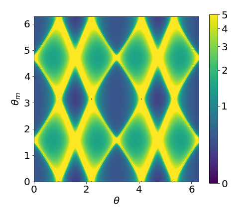
For each observed frequency channel and possible pair, we create an emission profile over the period of the magnetar rotation that includes no emission when . We calculate a time-integrated flux density, and we marginalize these flux densities at each channel over all . Figure 6 shows an example at 10 GHz of the influence of and on the angular term that includes time-averaging including times when . We also plot the net result of the marginalization over these unknown angles versus frequency and equivalent axion mass. These time-averaged and angle-marginalized angular terms are used in the calculation to place limits on (main Letter, Equation 4).