Cross-Global Attention Graph Kernel Network Prediction of Drug PrescriptionConference: Proceedings of the 11th ACM International Conference on Bioinformatics, Computational Biology and Health Informatics; September 21–24, 2020; Virtual Event, USAProceedings of the 11th ACM International Conference on Bioinformatics, Computational Biology and Health Informatics (BCB ’20), September 21–24, 2020, Virtual Event, USAPrice: 15.00DOI: 10.1145/3388440.3412459ISBN: 978-1-4503-7964-9/20/09CCS: Computing methodologies Artificial intelligenceCCS: Applied computing Health informatics
Abstract.
We present an end-to-end, interpretable, deep-learning architecture to learn a graph kernel that predicts the outcome of chronic disease drug prescription. This is achieved through a deep metric learning collaborative with a Support Vector Machine objective using a graphical representation of Electronic Health Records. We formulate the predictive model as a binary graph classification problem with an adaptive learned graph kernel through novel cross-global attention node matching between patient graphs, simultaneously computing on multiple graphs without training pair or triplet generation. Results using the Taiwanese National Health Insurance Research Database demonstrate that our approach outperforms current start-of-the-art models both in terms of accuracy and interpretability.
Keywords:
Health informatics; Predictive model; Deep Graph Kernel Learning; Graph kernel1. Introduction
Outcome prediction of chronic disease drug prescription is a preeminent yet unsolved problem. Chronic diseases are a major cause of illness in the United States11 1 https://www.cdc.gov/chronicdisease/index.htm and a top ten cause of death in Taiwan22 2 https://www.mohw.gov.tw/cp-4650-50697-2.html. Chronic disease drug prescription aims to reduce patient risk for severe comorbidities and complications. Prescribing such medication is difficult as long-term disease progression and numerous other factors complicate treatment plan design. On the other hand, the availability of Electronic Health Records (EHRs), providing historical medical road-maps for patients, enable the development of intelligent predictive systems for drug prescription (Pathak et al. 2013; Alphs-Jackson et al. 2011).
Various EHR modelling approaches, including electronic phenotyping (e.g., feature extraction) (Yadav et al. 2017) and highly-accurate deep learning models (e.g., representation learning) (Miotto et al. 2016), support such analytical tasks. For example, Recurrent Neural Networks (RNN) (Bajor and Lasko 2016) model time series medical data. However, interpretability concerns associated with deep learning approaches, particularly in the medical domain, limit their use. Notwithstanding, the trade-off to achieve high accuracy and high interpretability remains.
Many studies introduce attention-based RNN models to improve interpretability (Choi et al. 2016b; Ma et al. 2017). However, the majority of efforts rely on publicly available datasets or on a collaborating hospital’s EHR system where patient demographic information is mostly uniform. Unfortunately, this uniformity of data fails to exist when developing approaches for real-world, integrated EHR systems (e.g., insurance claim-based EHR systems). On this occasion, highly temporally dependent data attributes with high noise and variance often induce model over-fitting. Such a problem is addressed in (Yao et al. 2019a; Yao et al. 2019b) with a proposed graph-kernel EHR predictive model, yet they only consider a single medication with immediate outcome observations. For chronic diseases, long-term disease progression coupled with EHR complexity complicates the effort. We surmise that attention-based deep learning models and handcrafted kernel computations are limited to handle complex EHR under long-term disease progression. As discussed in (Yao et al. 2019b), the increased divergence and noise on data attributes over-fits the deep learning model and defeats the handcrafted kernel.
We propose a cross-global attention graph kernel network to learn optimal graph kernels on a graphical representation of patient EHRs. We term "cross-global" to delineate pairwise-less "cross" graph node attention and its "global" attention graph pooling. The novel cross-global attention node matching automatically captures relevant information in biased long-term disease progression. In contrast to attention-based graph similarity learning (Bai et al. 2019; Li et al. 2019; Al-Rfou et al. 2019) that relies on a pairwise comparisons of training pairs or triplets, our matching is performed on a batch of graphs simultaneously by a global cluster membership assignment. This is accomplished without the need to generate training pairs or triplets for pairwise computations and seamlessly combines classification loss. The learning process is guided by cosine distance. The resulting kernel, compared to its Euclidean distance counterpart, has better noise resistance under a high dimension space (Calin and Chang 2009; Calin et al. 2010). Unlike distance metric learning (Hadsell et al. 2006; Schroff et al. 2015) and aforementioned graph similarity learning, we align our learned distance and graph kernel to a classification objective. We formulate an end to end training by jointly optimizing contrastive and kernel alignment loss with a Support Vector Machine (SVM) primal objective. Such a training procedure encourages node matching and similarity measurement to produce ideal classification, providing interpretation on prediction. The resulting kernel function can be directly used by an off-the-shelf kernelized classifier (e.g., scikit-learn SVC 33 3 https://scikit-learn.org/stable/modules/svm.html). The cross-global attention node matching and kernel-based classification makes it interpretable in both knowledge discovery and prediction case study.
We evaluate our model using a country-wide population, claim-based database from Taiwan; the National Health Insurance Research Database (NHIRD). We formulate the chronic disease drug prediction task as a binary graph classification problem. An optimal graph kernel learned through cross-global attention graph kernel network is used to perform classification on a kernel SVM. Experimental results demonstrate that our proposed method outperforms current state-of-the-art approaches as well as providing model interpretability. Analysis on node matching between patient graphs indicates how our cluster membership assignment can generate effective node matching without explicit pairwise computation. We also demonstrate superior interpretability over node matching on most similar cases and support vectors, serving as knowledge and information discovery on prediction. We are the first to combine pairwise-less graph kernel learning and classification objective in an end to end learning procedure for medical practice. Our approach is under clinical used and evaluation.
Our contributions are as follows:
- •
We propose an end-to-end, deep metric learning based framework to learn an optimal graph kernel on highly noisy EHR data.
- •
We present a pairwise-less attention-based node matching operation and metric-learning process without the need to generate training pairs or triplets to perform pairwise similarity measurement, seamlessly combining SVM objectives.
- •
We experiment with large-scale, real-world, long-term span medical data to demonstrate our effectiveness together with interpretability, surpassing all state-of-the-art baselines.
- •
We provide a clinically-vetted approach.


2. Related work
Most drug prescription prediction tasks focus on Adverse Drug Reactions (ADRs) or medication errors (Aronson 2009; Yates et al. 2015; Xiao et al. 2017; Nguyen et al. 2013) while other efforts discuss the effectiveness of drug prescription for a given disease diagnosis (Alphs-Jackson et al. 2011; Kang et al. 2015). The approaches mainly discuss ADRs and specific disease target information and are unable to utilize EHR for outcome prediction and complex disease progression modeling from medical history.
Despite traditional electronic phenotyping (Yadav et al. 2017), representation learning on EHR benefits from deep learning models. Most efforts use deep architectures to learn EHR embeddings via Multi-layer Perceptron (MLP) (Miotto et al. 2016; Choi et al. 2016a), Convolutional Neural Network (CNN) (Che et al. 2017) or Recurrent Neural Network (RNN) to model time series medical information (Bajor and Lasko 2016). An Attention-based model was also proposed to address model interpretability (Choi et al. 2016b; Ma et al. 2017; Choi et al. 2017; Mullenbach et al. 2018; Xie et al. 2019). Recently, BERT trained on clinical language (Clinical BERT) was introduced to support various fine-tuning tasks such as hospital readmission prediction (Huang et al. 2019; Alsentzer et al. 2019). However, most efforts concentrate on medical code prediction and medical concept embedding and do not directly map onto a drug prediction task. Moreover, the model over-fitting and interpretability trade-off still remains unsolved. In (Yao et al. 2019a; Yao et al. 2019b), a graph kernel approach is developed to predict outcomes of a drug prescription for a given disease diagnosis, which achieves state-of-the-art results. However, as mentioned in Section 1 and evaluated in Section 5.4, chronic diseases are not considered in the model, leading to under-performance prediction. Overall, the EHR prediction task on drug prescription is not fully investigated.
3. Prediction Task on chronic disease drug prescription
3.1. EHR Patient Graph
We formulate a patient’s EHR as a Directed Acyclic Graph (DAG) following the definition in (Yao et al. 2019a), for which each node represents a medical event, and an edge between two nodes represents an ordering with the time difference as edge weight (e.g., days). The demographic information of the patient, e.g., gender, connects to the first medical event with age as an edge weight. Figure 2 describes an example patient graph. As in (Yao et al. 2019a), we only use gender and age as demographic information to simplify the model. All node labels are one-hot encoded.
3.2. Success and Failure cases
To define the success or failure of a treatment plan 44 4 Since chronic diseases require a set of drug prescriptions with necessary adjustment per disease condition, we use the term treatment plan and drug prescription interchangeably. for a chronic disease, we follow the guideline published by the National Medical Association for selected chronic diseases (Chiang et al. 2015; Li et al. 2017; dia 2020). Generally, an observation window is defined after a treatment period to monitor whether the given treatment plan achieves its treatment objective (e.g., no severe complication occurrence in 5 years). Given a chronic disease diagnosis, a treatment is considered a failure if the patient is diagnosed with a selected severe complication or comorbidity within the post treatment observation window. Otherwise, the treatment is considered a success. Figure 3 illustrates this criterion. Due to the chronic disease long-term progression where past factors are potentially decisive, all medical histories are included prior to the first diagnosis date. We treat each case as a set of medical records from a patient’s EHR as in Figure 1. The terms, patient and case, are used interchangeably.



3.3. Prediction Framework
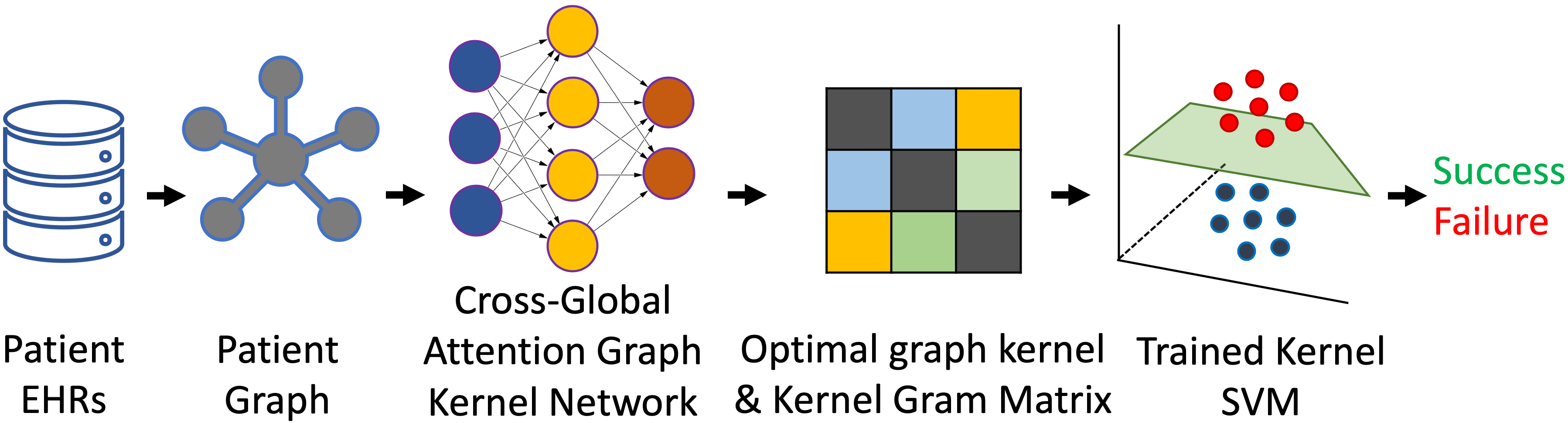
We formulate our prediction task as a binary graph classification on graph-based EHR using a kernel SVM. Although similar to (Yao et al. 2019a), we differentiate our approach by learning a graph kernel, not handcrafting one. Given a set of success and failure case patient graphs , a deep neural network learns an optimal graph kernel k. Then, the prediction for success and failure is performed by a kernel SVM using a kernel gram matrix K such that where . For an incoming patient, we create a patient graph based on the concatenation of patient’s medical history, current diagnosis, and treatment plan. Then, we determine the kernel value between and all training examples , and perform prediction through a kernel SVM. The proposed system is illustrated in Figure 4.
4. Cross-Global Attention Graph Kernel Network
Our Cross-Global Attention Graph Kernel Network learns an end-to-end deep graph kernel on a batch of graphs. This is accomplished through cross-global attention node matching without an explicit pairwise similarity computation. Given a batch of input graphs with batch size , we embed their nodes into a lower dimensional space, where node structures and attribute information are encoded in dense vectors. A graph level embedding is then produced by a graph pooling operation on node level embedding via cross-global attention node matching. We calculate the batch-wise cosine distance and generate a kernel gram matrix on the entire batch of resulting graph embedding. Finally, the network loss is computed with contrastive loss, kernel alignment, and SVM primal objective. An overview of cross-global attention graph kernel network is illustrated in Figure 5. The remainder of this section details this process.
4.1. Graph Embedding
4.1.1. Graph Convolutional Networks
Graph Convolutional Networks (GCN) (Kipf and Welling 2017) perform 1-hop neighbor feature aggregation for each node in a graph. The resulting graph embedding is permutation invariant when a pooling operation is properly chosen. Given an number nodes patient graph with node attribute one-hot vector matrix , where denotes the total number of medical codes in EHRs, and a weighted adjacency matrix , we use GCN to generate a node level embedding with embedding size as follows:
| (1) |
where is the diagonal node degree matrix of defined with , is the adjacency matrix with self-loops added, is a trainable weight matrix, and is a non-linear activation function such as . The embedding can be an input to another GCN, creating stacked multiple graph convolution layers:
| (2) |
where is the node embedding after the GCN operation, and is the trainable weight associated with the GCN layer. The resulting node embedding contains k-hop neighborhood structure information aggregated by graph convolution layers.
4.1.2. Higher-order graph information
To capture longer distance nodes and preserve their hierarchical multi-hop neighborhood information as in (Chen et al. 2019), we stacked multiple GCN layers55 5 Assuming the dimension of all layers’ trainable weight matrices are the same and concatenated all layer’s outputs where . The concatenated node embedding might be very large and could potentially cause a memory issue for subsequent operations. To mitigate such drawbacks, we perform a non-linear transformation on by a trainable weight and a ReLU activation function as follows:
| (3) |
To produce the graph level embedding, instead of using another type of pooling operation (Zhang et al. 2018; Ying et al. 2018; Lee et al. 2019), we propose cross-global attention node matching and its derived attention based pooling.
4.2. Cross-Global Attention Node Matching
Node matching between graphs is computed via a pairwise node similarity measurement. This optimizes a distance metric-based or KL-divergence loss on the graph pairs or triplets (Bai et al. 2019; Li et al. 2019; Al-Rfou et al. 2019) necessitating vast training pairs or triplets to capture the entire global characteristics. One way to avoid explicit pair or triplet generation utilizes efficient batch-wise learning via optimizing classification loss (Wen et al. 2016; Qian et al. 2019). However, pairwise node matching in a batch-wise setting is problematic due to graph size variability.
To address this issue, we propose a novel batch-wise attention-based node matching scheme, a.k.a., cross-global attention node matching. The matching scheme learns a set of global node clusters and computes the attention weight between each node and the representation associated with its membership cluster. The pooling operation based on its attention score to global cluster performs a weighted sum on nodes to derive a single graph embedding.
4.2.1. Global Node Cluster Learning and Cluster Representation Query
Given node embedding from the last GCN layer and transformation after concatenation in Equation 3, we define as a trainable global node cluster matrix with clusters and dimension features sized to provide an overall representation of its membership nodes. Here, we define membership assignment for and as follows:
| (4) |
where Sparsemax (Martins and Astudillo 2016) is a sparse version Softmax, that outputs sparse probabilities. It can be treated as a sparse soft cluster assignment. We can interpret as a cluster membership identity with dimension feature representation. We further define the query of nodes’ representation in their belonging membership cluster:
| (5) |
where denotes a queried representation for each node in from their belonging membership cluster.
As described in Figure 6, matching can be treated as retrieving cluster identity from global node clusters, and similar nodes are assigned to a similar or even the same cluster membership identity. To construct a better cluster, we add an auxiliary loss by minimizing the reconstruction error, which is similar to Non-negative Matrix Factorization (NMF) clustering in (Ding et al. 2005) as:
| (6) |
4.2.2. Pooling with Attention-based Node Matching
The intuition of pairwise node matching is to assign higher attention-weight to those similar nodes. In other words, matching occurs when two nodes are highly similar, closer to each other than to other possible targets. Following this idea, we observe that two nodes are matched if they have similar or even identical cluster membership. The higher the similar membership identity, the higher the degree of node matching. In addition, a cluster is constructed by minimizing the reconstruction error between the original node and the query representation . A node with high reconstruction error means no specific cluster assignment and further lowers the chance to match other nodes. This can be measured by using entry-wise similarity metrics (e.g., cosine similarity) between and its respective query representation . Higher similarity between them reveals better reconstruction quality and potential to match other nodes. Based on these observations, we design the cross-global attention node matching pooling, where a node similar to the representation in its cluster membership should receive higher attention weight, as follows:
| (7) |
where is the attention weight for each node, Softmax is applied to generate importance among nodes by using Sim, a similarity metric (e.g., cosine similarity), and the resulting pooling is the weighted sum of node embeddings that compress higher order structure and node matching information from other graphs. Matching and cluster assignment membership is illustrated in Figure 6.

4.3. Graph Kernel
Given a graph pair with their graph level embeddings , we define the graph kernel as follows:
| (8) |
where is a cosine distance and is the Euclidean distance. As usual, is a standard inner product. can be either or . The resulting kernel function is positive definite since is positive definite for any real number (Calin et al. 2010)66 6 Due to the space limits, we do not include the complete proof here. It can be easily proved by the definition of positive definiteness with the same derivation in (Calin et al. 2010; Chang et al. 2018).. Cosine distance enjoys benefits in more complex data representations. Euclidean distance considers vector magnitude (i.e., norm) during measurement which is not sufficiently sensitive to highly variant features such as long-term disease progressions. Moreover, cosine distance can measure objects on manifolds with nonzero curvature such as spheres or hyperbolic surfaces. In general, Euclidean distance can only be applied to local problems which may not be sufficient to express complex feature characteristics (Calin and Chang 2009). The resulting cosine guided kernel is more expressive, and thus, capable of performing implicit high dimensional mapping (Calin et al. 2010).
4.4. Training
Given a batch of input graphs and their class labels where , we get their graph level embeddings for the entire batch via shared weight GCN with cross-global node matching pooling. To support graph size variation within a batch, we concatenate their feature matrices and combine their adjacency matrices into a sparse block-diagonal matrix. Each block corresponds to an adjacency matrix of a graph in the batch. The resulting concatenated feature matrix and block-diagonal matrix are treated as a single graph, so all operations (e.g., GCN and pooling) can perform simultaneously on batch-wise graphs. Then, we calculate their batch-wise distance matrix and batch-wise kernel gram matrix . The model can be trained by mini-batch Stochastic Gradient Descent (SGD) without training pair and triplet generation. To learn an optimal graph embedding, which results in an optimal graph kernel, we optimize it by contrastive loss (Hadsell et al. 2006) with a margin threshold :
| (9) |
and kernel alignment loss (Cristianini et al. 2002):
| (10) |
where denotes the frobenius inner product, K is a batch-wise kernel gram matrix, and where if else . We believe that a good distance-metric induces a good kernel function and vice versa. So, we learn the graph kernel jointly through optimal cosine distance between graphs via contrastive loss with an optimal graph kernel through kernel alignment loss.
To align a learned embedding, distance, and kernel to the classification loss in end-to-end training, we incorporate the SVM primal (Chapelle 2007) objective with squared hinge loss function into our objective:
| (11) |
where is a user defined regularization constant and is a trainable coefficient weight vector. The following is the final model optimization problem formulation:
| (12) |
where denotes a set of all trainable variables in graph embedding and is a trainable coefficient weight vector for SVM. Since the training is done by mini-batch SGD, the SVM objective is only meaningful for a given batch. Namely, gradient for in SVM are only relevant for the current batch update as the SVM objective is dependent on the input kernel gram matrix. When training proceeds to the next batch, the kernel gram matrix is different, and the optimized is inconsistent with the last batch status. To resolve this inconsistent weight update problem, we treat SVM as a light-weight auxiliary objective (e.g., regularization), encouraging the model to learn an effective graph kernel. In this case, we first perform a forward pass through graph kernel network, then we train the SVM by feeding in the kernel gram matrix from the forward pass output until convergence. The positive definiteness of the kernel function guarantees SVM convergence77 7 Due to page limit, we do not show convergence analysis. However, averaged iterations for SVM is 18.. Once the SVM is trained, we treat as a model constant, and now acts as a regular loss function. The gradient of can be computed through , , and , and the model can perform backpropagation to update .
5. Experiments
5.1. Dataset
We evaluate our model on real-world EHRs, a subset of the Taiwanese National Health Insurance Research Database (NHIRD) 88 8 https://nhird.nhri.org.tw/en/, which contains over a 20-year complete medical history for one-million randomly sampled de-identified patients. NHIRD composes reimbursement related registration files and original claim data for hospitals and clinics that enroll in the National Health Insurance (NHI) program. The ICD9-CM99 9 International Classification of Diseases, 9th Revision, Clinical Modification code indicates the diagnosed disease and the ATC1010 10 Anatomical Therapeutic Chemical code is used for drug prescription. Institutional Review Board (IRB) approvals for our research were granted by all associated institutions.
The three most prevalent chronic diseases in Taiwan, namely, hypertension, hyperlipidemia, and diabetes, are selected. Their treatments primarily rely on a long-term treatment plan including multiple drug prescriptions to control disease progression. The effectiveness of treatment depends on the risk level of possible future severe comorbidities and complications after receiving the treatment plan for several years. The goal is to predict the success or failure for the given drug prescriptions during the treatment period of a chronic disease diagnosis. According to our collaborating medical doctors and to published treatment guidelines of hypertension (Chiang et al. 2015), hyperlipidemia (Li et al. 2017), and diabetes (dia 2020), we define success and failure cases for each disease by the following steps:
- (1)
Locate the first chronic disease diagnosis date .
- (2)
Set year observation window for treatment plan.
- (3)
Set treatment plan end date .
- (4)
Set year observation window for outcome.
- (5)
Set outcome observation end date .
- (6)
If no selected severe comorbidities and complications diagnosis exist between and , the case is defined successful, otherwise, a failure.
We use the patient’s entire medical history (a.k.a., clinical visits) from the first medical record to to create the patient graphs. We set for 1 year and for 10 years. For each medical event, we extract all diagnosis ICD-9 codes and drug prescription ATC codes. Table 2 summarizes the dataset statistic, and Table 1 lists all selected complication ICD-9 codes for each disease.
| Disease | Selected Complication ICD9 Codes | ||||||
|---|---|---|---|---|---|---|---|
| Hypertension |
| ||||||
| Hyperlipidemia |
| ||||||
| Diabetes |
|
| Disease | Hypertension | Hyperlipidemia | Diabetes |
| ICD9 Codes | 401.* | 272.* | 250.* |
| # of patient | 235,695 | 123,380 | 131,997 |
| # of failure | 104,936 (45%) | 26,043 (21%) | 34,414 (26%) |
| # of success | 130,759 (55%) | 97,337 (79%) | 97,583 (74%) |
| Max # nodes | 33,497 | 19.159 | 15,454 |
| Min # nodes | 3 | 3 | 3 |
| Avg # nodes | 220 | 285 | 374 |
| Max # edges | 87,852 | 52,750 | 57422 |
| Min # edges | 2 | 2 | 2 |
| Avg # edges | 561 | 620 | 891 |
| Hypertension | Hyperlipidemia | Diabetes | |||||||
| Model | ACC | AUC | F1 | ACC | AUC | F1 | ACC | AUC | F1 |
| CGA-GK-Cosine (Our) | 0.7417 | 0.7361 | 0.7371 | 0.8702 | 0.7428 | 0.7727 | 0.7804 | 0.6602 | 0.6758 |
| CGA-GK-Euclidean (Our) | 0.7337 | 0.7278 | 0.7290 | 0.8507 | 0.6798 | 0.7153 | 0.7613 | 0.5920 | 0.5970 |
| MGKF | 0.6990 | 0.7025 | 0.6973 | 0.7200 | 0.7043 | 0.6698 | 0.7250 | 0.6354 | 0.6404 |
| WL-Kernel-SVM | 0.7101 | 0.6968 | 0.6982 | 0.8293 | 0.6092 | 0.6304 | 0.7625 | 0.5911 | 0.5955 |
| DGCNN | 0.6954 | 0.6895 | 0.6894 | 0.8290 | 0.6338 | 0.6518 | 0.7536 | 0.5871 | 0.5914 |
| ClinicalBERT | 0.7132 | 0.6996 | 0.6434 | 0.8510 | 0.6808 | 0.5215 | 0.7720 | 0.6484 | 0.4718 |
| Retain | 0.6580 | 0.6537 | 0.6174 | 0.8340 | 0.6908 | 0.5337 | 0.7657 | 0.6369 | 0.4529 |
| Dipole | 0.6603 | 0.6805 | 0.6782 | 0.8180 | 0.5943 | 0.3259 | 0.7553 | 0.5540 | 0.2338 |
| LSTM | 0.6960 | 0.6607 | 0.5250 | 0.7920 | 0.6267 | 0.3988 | 0.7283 | 0.5497 | 0.2598 |
| CNN | 0.7170 | 0.6999 | 0.6323 | 0.8320 | 0.6920 | 0.5359 | 0.7317 | 0.6481 | 0.4679 |
| Med2Vec | 0.6864 | 0.6681 | 0.5847 | 0.8167 | 0.6593 | 0.4575 | 0.7524 | 0.2698 | 0.5805 |
| Deep Patient | 0.6560 | 0.6443 | 0.5835 | 0.7980 | 0.5295 | 0.1217 | 0.7280 | 0.5395 | 0.1905 |
| LR | 0.7220 | 0.7083 | 0.6532 | 0.8368 | 0.6417 | 0.4401 | 0.7483 | 0.5371 | 0.1658 |
| SVM | 0.6909 | 0.6738 | 0.6016 | 0.8168 | 0.6939 | 0.5252 | 0.7294 | 0.6329 | 0.4544 |
| RF | 0.7266 | 0.7188 | 0.6774 | 0.8424 | 0.6507 | 0.4609 | 0.7631 | 0.3066 | 0.5811 |
5.2. Baselines
Three types of baselines are selected to compare our model performance: Deep learning based, graph classification based, and traditional based.
Deep learning based approaches:
- •
Deep Patient (Miotto et al. 2016). Deep Patient utilizes a three-layer stacked denoising autoencoder to perform unsupervised representation learning on EHRs with Random Forest to predict future diagnosis.
- •
LSTM (Bajor and Lasko 2016). A LSTM model with word embedding to encode time series clinical measurements in EHRs is used to predict future medical code diagnosis.
- •
Med2Vec (Choi et al. 2016a). Med2Vec uses multi-layer perceptron to learn interpretable code and visit embedding based on the skip-gram model. The code level embedding is learned first, and the resulting embedding is concatenated with demographic information to form visit level embedding.
- •
Retain (Choi et al. 2016b). It is a RNN using GRU with a two-level reverse time attention mechanism, which offer interpretation to select influential past visits contributing to the final prediction.
- •
CNN (Che et al. 2017). This model uses a 1D-CNN to learn EHRs temporal embedding matrix representation to capture local and short temporal dependency in EHRs for risk prediction.
- •
Dipole (Ma et al. 2017). It is a bidirectional RNN with three different attention mechanisms, proposed to calculate attention weights for each patient visit: general, concatenation-based, and location-based. In our experiment, we use multiplicative attention (Luong et al. 2015) to compute attention weight due to memory constraints.
- •
Clinical BERT (Alsentzer et al. 2019). In their work, a pre-trained clinical language model trained by the state-of-the art BERT model is created. We use their Clinical BERT as the BERT base model to train our language model on NHIRD. For each patient case, we concatenate all medical codes from all visits into a single document. Then, we fine-tune it on our prediction task.
Graph based approaches:
- •
WL-Kernel-SVM (Shervashidze et al. 2011). Here, we use Weisfeiler-Lehman subtree graph kernel to compute a pairwise kernel gram matrix on all patient graphs. Then, a kernel SVM is used to perform graph classification.
- •
DGCNN (Zhang et al. 2018). It is an end-to-end graph classification model by graph convolution networks with a sort pooling layer to derive permutation invariant graph embeddings. 1D-CNN then extracts features along with full-connected layer for graph classification task on patient graphs.
- •
MGKF (Yao et al. 2019b). In their work, a deep learning architecture to learn the fusion representation of three types of graph kernels is proposed. They perform an antibiotics-based disease drug prediction task. In our experiment, we replace their shortest path kernel with Weisfeiler-Lehman subtree graph kernels on patient graphs to avoid insufficient memory and a forever running time issue for shortest path kernel.
Traditional approaches 1111 11 All patient cases are represented as documents with one-hot encoding containing all medical codes from all visits.:
- •
Linear Support Vector Machine (SVM).
- •
Logistic Regression (LR).
- •
Random Forest (RF).
5.3. Evaluation Setup
Accuracy (ACC), F1-score (Macro F1), and the area under the receiver operating characteristic curve (AUROC) are used as our evaluation metrics. For each disease, we randomly divide our datasets into training, validation, and testing sets in an 80:10:10 ratio. We notice the data imbalance as shown in Table 2. To reflect real-world clinical practice, we do not use any data balancing techniques and keep data imbalance. All parameters for all evaluated models are fine tuned via the validation set. The pairwise t-test with a p-value set to 0.05 is used to reject the null-hypothesis to assess the statistical significance of our proposed model. Our solution statistically significantly differs from previous efforts. For our proposed model architecture, we set 6 layers GCN with output dimension 256 and ReLU activation function. We set the number of global node clusters to 256 and the contrastive loss margin threshold . We use Tensorflow-Keras to implement our proposed model architecture. For SVM training, we set 100 iterations with early stopping and an regularization constant . For the training stage, we use the Adam optimizer with an initial fixed learning rate set to 0.0005 with 128 batch size and train for 10 epochs with early stopping criteria. For the graph classification stage, we use classical kernel SVM from scikit-learn (Pedregosa et al. 2011) and set the regularization constant . All experiments are executed on an Intel Core i7 CPU, with 64GB memory and one Nvidia 1080 Ti GPU.
5.4. Experimental Results
Table 3 shows that our proposed approach (CGA-GK-Cosine) consistently outperforms all baseline approaches on all evaluation metrics. Specifically, all baselines are affected by data imbalance and receive high Accuracy and AUC but low F1 scores, particularly in the imbalance hyperlipidemia and diabetes dataset as depicted in Table 2. Data imbalance is common in real-world clinical practice, and it is critical when developing medical applications. It is undesirable to prescribe a false predicted success drug treatment, which may lead to severe disease progression or fatality. Furthermore, NHIRD, a real-world claim-based EHR database, is known to have highly biased medical records along with unpredictable and irregular patterns such as (1) Record splitting: multiple same diagnosis records with different drug prescription (2) Reimbursement trick: only record higher reimbursement drug or disease (3) Patient shopping behavior: multiple same disease diagnosis without drug prescription on the same date, and medical events from all of these conditions are pointless.
Our approach is insensitive to data imbalance and yields the highest F1 score, highlighting its ability to learn a meaningful and noise resistant graph kernel since the prediction is conducted purely by traditional kernel SVM. The high F1 score also demonstrates that CGA-GK-Cosine outperforms CGA-GK-Euclidean, highlighting the advantage of cosine distance over Euclidean distance. This result confirms our hypothesis that cosine distance captures micro differences in feature dimension and is relatively insensitive to the highly biased dataset, as compared to its counterparts.
Looking at different baseline groups, the graph-based approach outperforms all other baselines on F1, revealing the usefulness for graphs as a modeling tool under real world data imbalance situation. The graph kernel approaches show the effectiveness of similarity-based classification to overcome highly variant and imbalanced medical records. For deep learning baselines, we observe they all tend to predict drug treatment as success, which leads to low F1 for all tasks. It is even worse on RNN based models due to their over-fitting on the majority class. We also hypothesize that pre-trained fine-tuned BERT language model is not suitable for drug prediction task, as its training objective is not aligned to disease progression.
For most other research efforts, the datasets used are either from a collaborating hospital or public dataset, namely MIMIC31212 12 We’re not using MIMIC3 since it doesn’t contain enough medical history to monitor chronic disease outcome., with a significantly shorter medical history per patient and much less biased data records. Consequently, the model developed on such datasets fails to comply with NHIRD and suffers from over-fitting under an imbalanced situation. Traditional approaches are too shallow to learn meaningful representation; however, due to their simple learning process, they can avoid severe over-fitting and perform better than some deep learning approaches (e.g., Dipole, LSTM, and Deep Patient).
5.5. Cross-Global Attention Node Matching
We evaluate our proposed node cluster membership assignment based on how two identical graphs relate to each other under different node and edge removals. If two graphs are identical, they should match themselves symmetrically (e.g., the diagonal part). By randomly removing some node and edge labels, the matching result will change since the graph structure is changed. We select an identical patient graph from hypertension in Figure 7. Nodes of the same color indicate same cluster membership by selecting the largest dimension in their cluster membership label, which implies matching. The heatmap shows the full attention matrix on node matching which reveals a more complete view of their alignment.
In Figure 7(a), when we remove all node labels and edge connections, nodes do not match themselves. At this time, they are considered as differing graphs with different cluster membership assignments, although they are actually identical. By recovering some node labels and all edge connections in Figure 7(b), we can see their degree of alignment is increased. Finally, when all nodes and edges are recovered, their nodes are matched to themselves with the same cluster membership assignment. In Figure 7(c), we can see the matching is a symmetrical one-to-one alignment between all nodes in the diagonal. Results suggest that our cross-global attention node matching, which is computed on batch of graphs simultaneously, can successfully provide an effective matching without explicit pairwise graph comparisons.


5.6. Model Interpretation
Our proposed method enjoys three types of interpretations: (1) patient graph interpretation, (2) most similar case on cause of prediction, and (3) knowledge discovery on support vectors:

Patient Graph Interpretation
We can use the cross-global attention score on each node to discover important disease diagnoses and drug prescriptions on a per patient basis. The higher the score, namely the better matching to others, the more important the node is in the similarity computation. The patient graph in Figure 8 is easily understood by medical doctors due to their graphical representation. Together with high attentive node visualization, they provide investigative direction and background knowledge on patient disease progression.
Most Similar Case on Cause of Prediction
Kernel measures the similarity between two cases patient graph ; we can infer the most similar case for by finding the highest kernel value. With cross-global attention node matching in Figure 9, one sees how these two graphs match each other. The graphical representation highlights common disease progression related to matched nodes. The insights on how these two patient cases are similar guides medical doctors as to the cause of why the given treatment is a success or failure.


Knowledge Discovery on Support Vectors
Finally, we consult a set of top support vectors from the kernel SVM, which receive top maximum dual coefficients 1313
13
Refer (Chapelle 2007) for SVM dual formulation., interpreting the overall importance to assign a class label during SVM training. Combining this with the previous two types of interpretation techniques, we are able to discover knowledge among overall disease patterns for a success or failure treatment plan.
6. Conclusion and Future Work
The highly biased and variant nature of real-world EHR coupled with the long-term disease progression behavior of chronic diseases challenge the development for predictive models in clinical decision support. Many proposed prior efforts address such difficulty, yet none succeeded nor earned clinical deployment. Deep learning models tend to over-fit on real-world EHR with highly biased long-term time progression medical patterns, worse yet when data imbalance exists. Furthermore, interpretability measures still demand refinement due to the opaqueness of deep neural networks.
Accordingly, we proposed a deep learning model, namely, cross-global attention graph kernel network, to learn an optimal graph kernel and achieve state-of-the-art prediction accuracy on highly biased and imbalanced real-world EHR. The cosine distance guided the learning process with SVM primal objective learning an optimal noise resistant graph kernel. The novel cross-global attention node matching efficiently captures important graph structure without explicit pairwise comparisons. The classification results outperform all state-of-the-art baselines simply using a traditional kernel SVM. Three types of interpretation techniques can work cooperatively to maximize model interpretability. We also notice that cosine distance has interesting properties, specifically, in sub-Riemannian geometry. This is a very active research direction in partial differential equations with many applications in control theory, such as self-driving automobiles and the stochastic process of heat flows (Calin and Chang 2009; Calin et al. 2010). We plan to study the sub-Riemannian geometry that can be applied to model EHR patient similarity.
Our approach predicts chronic disease drug prescription outcome for long-term disease progression, exceeding the performance of state-of-the-art in all evaluation metrics, while providing interpretability. It was intentionally designed in coordination with and is under current use and assessment by medical clinicians in diverse clinical practices.
References
- (1)
- dia (2020) 2020. Introduction: Standards of Medical Care in Diabetes—2020. Diabetes Care (2020).
- Al-Rfou et al. (2019) Rami Al-Rfou, Bryan Perozzi, and Dustin Zelle. 2019. Ddgk: Learning graph representations for deep divergence graph kernels. In The World Wide Web Conference. 37–48.
- Alphs-Jackson et al. (2011) Hannah Alphs-Jackson, John Cashy, Ophir Frieder, and Anthony J Schaeffer. 2011. Data mining derived treatment algorithms from the electronic medical record improve theoretical empirical therapy for outpatient urinary tract infections. The Journal of urology 186, 6 (2011), 2257–2262.
- Alsentzer et al. (2019) Emily Alsentzer, John Murphy, William Boag, Wei-Hung Weng, Di Jindi, Tristan Naumann, and Matthew McDermott. 2019. Publicly Available Clinical BERT Embeddings. In Proceedings of the 2nd Clinical Natural Language Processing Workshop. 72–78.
- Aronson (2009) JK Aronson. 2009. Medication errors: what they are, how they happen, and how to avoid them. QJM : monthly journal of the Association of Physicians 102, 8 (2009), 513–521.
- Bai et al. (2019) Yunsheng Bai, Hao Ding, Song Bian, Ting Chen, Yizhou Sun, and Wei Wang. 2019. Simgnn: A neural network approach to fast graph similarity computation. In Proceedings of the Twelfth ACM International Conference on Web Search and Data Mining. 384–392.
- Bajor and Lasko (2016) Jacek M Bajor and Thomas A Lasko. 2016. Predicting medications from diagnostic codes with recurrent neural networks. (2016).
- Calin and Chang (2009) Ovidiu Calin and Der-Chen Chang. 2009. Sub-Riemannian Geometry: General Theory and Examples. Cambridge University Press.
- Calin et al. (2010) Ovidiu Calin, Der-Chen Chang, Kenro Furutani, and Chisato Iwasaki. 2010. Heat kernels for elliptic and sub-elliptic operators. Springer.
- Chang et al. (2018) Der-Chen Chang, Ophir Frieder, and Hao-Ren Yao. 2018. On bochner’s theorem and its application to graph kernels. Journal of Nonlinear and Convex Analysis 19, 12 (2018), 2135–2151.
- Chapelle (2007) Olivier Chapelle. 2007. Training a support vector machine in the primal. Neural computation 19, 5 (2007), 1155–1178.
- Che et al. (2017) Zhengping Che, Yu Cheng, Zhaonan Sun, and Yan Liu. 2017. Exploiting convolutional neural network for risk prediction with medical feature embedding. arXiv preprint arXiv:1701.07474 (2017).
- Chen et al. (2019) Fengwen Chen, Shirui Pan, Jing Jiang, Huan Huo, and Guodong Long. 2019. DAGCN: dual attention graph convolutional networks. In 2019 International Joint Conference on Neural Networks (IJCNN). IEEE, 1–8.
- Chiang et al. (2015) Chern-En Chiang, Tzung-Dau Wang, Kwo-Chang Ueng, Tsung-Hsien Lin, Hung-I Yeh, Chung-Yin Chen, Yih-Jer Wu, Wei-Chuan Tsai, Ting-Hsing Chao, Chen-Huan Chen, et al. 2015. 2015 guidelines of the Taiwan Society of Cardiology and the Taiwan Hypertension Society for the management of hypertension. Journal of the Chinese Medical Association 78, 1 (2015), 1–47.
- Choi et al. (2016a) Edward Choi, Mohammad Taha Bahadori, Elizabeth Searles, Catherine Coffey, Michael Thompson, James Bost, Javier Tejedor-Sojo, and Jimeng Sun. 2016a. Multi-layer representation learning for medical concepts. In Proceedings of the 22nd ACM SIGKDD International Conference on Knowledge Discovery and Data Mining. ACM, 1495–1504.
- Choi et al. (2017) Edward Choi, Mohammad Taha Bahadori, Le Song, Walter F Stewart, and Jimeng Sun. 2017. GRAM: graph-based attention model for healthcare representation learning. In Proceedings of the 23rd ACM SIGKDD International Conference on Knowledge Discovery and Data Mining. ACM, 787–795.
- Choi et al. (2016b) Edward Choi, Mohammad Taha Bahadori, Jimeng Sun, Joshua Kulas, Andy Schuetz, and Walter Stewart. 2016b. Retain: An interpretable predictive model for healthcare using reverse time attention mechanism. In Advances in Neural Information Processing Systems. 3504–3512.
- Cristianini et al. (2002) Nello Cristianini, John Shawe-Taylor, Andre Elisseeff, and Jaz S Kandola. 2002. On kernel-target alignment. In Advances in neural information processing systems. 367–373.
- Ding et al. (2005) Chris Ding, Xiaofeng He, and Horst D Simon. 2005. On the equivalence of nonnegative matrix factorization and spectral clustering. In Proceedings of the 2005 SIAM international conference on data mining. SIAM, 606–610.
- Hadsell et al. (2006) Raia Hadsell, Sumit Chopra, and Yann LeCun. 2006. Dimensionality reduction by learning an invariant mapping. In 2006 IEEE Computer Society Conference on Computer Vision and Pattern Recognition (CVPR’06), Vol. 2. IEEE, 1735–1742.
- Huang et al. (2019) Kexin Huang, Jaan Altosaar, and Rajesh Ranganath. 2019. Clinicalbert: Modeling clinical notes and predicting hospital readmission. arXiv preprint arXiv:1904.05342 (2019).
- Kang et al. (2015) Seokho Kang, Pilsung Kang, Taehoon Ko, Sungzoon Cho, Su-jin Rhee, and Kyung-Sang Yu. 2015. An efficient and effective ensemble of support vector machines for anti-diabetic drug failure prediction. Expert Systems with Applications 42, 9 (2015), 4265–4273.
- Kipf and Welling (2017) Thomas N Kipf and Max Welling. 2017. Semi-supervised classification with graph convolutional networks. In International Conference on Learning Representations.
- Lee et al. (2019) Junhyun Lee, Inyeop Lee, and Jaewoo Kang. 2019. Self-Attention Graph Pooling. In International Conference on Machine Learning. 3734–3743.
- Li et al. (2019) Yujia Li, Chenjie Gu, Thomas Dullien, Oriol Vinyals, and Pushmeet Kohli. 2019. Graph Matching Networks for Learning the Similarity of Graph Structured Objects. In International Conference on Machine Learning. 3835–3845.
- Li et al. (2017) Yi-Heng Li, Kwo-Chang Ueng, Jiann-Shing Jeng, Min-Ji Charng, Tsung-Hsien Lin, Kuo-Liong Chien, Chih-Yuan Wang, Ting-Hsing Chao, Ping-Yen Liu, Cheng-Huang Su, et al. 2017. 2017 Taiwan lipid guidelines for high risk patients. Journal of the Formosan Medical Association 116, 4 (2017), 217–248.
- Luong et al. (2015) Minh-Thang Luong, Hieu Pham, and Christopher D Manning. 2015. Effective Approaches to Attention-based Neural Machine Translation. In Proceedings of the 2015 Conference on Empirical Methods in Natural Language Processing. 1412–1421.
- Ma et al. (2017) Fenglong Ma, Radha Chitta, Jing Zhou, Quanzeng You, Tong Sun, and Jing Gao. 2017. Dipole: Diagnosis prediction in healthcare via attention-based bidirectional recurrent neural networks. In Proceedings of the 23rd ACM SIGKDD international conference on knowledge discovery and data mining. ACM, 1903–1911.
- Martins and Astudillo (2016) Andre Martins and Ramon Astudillo. 2016. From softmax to sparsemax: A sparse model of attention and multi-label classification. In International Conference on Machine Learning. 1614–1623.
- Miotto et al. (2016) Riccardo Miotto, Li Li, Brian A Kidd, and Joel T Dudley. 2016. Deep patient: an unsupervised representation to predict the future of patients from the electronic health records. Scientific reports 6 (2016), 26094.
- Mullenbach et al. (2018) James Mullenbach, Sarah Wiegreffe, Jon Duke, Jimeng Sun, and Jacob Eisenstein. 2018. Explainable Prediction of Medical Codes from Clinical Text. In Proceedings of the 2018 Conference of the North American Chapter of the Association for Computational Linguistics: Human Language Technologies, Volume 1 (Long Papers). 1101–1111.
- Nguyen et al. (2013) Phung Anh Nguyen, Shabbir Syed-Abdul, Usman Iqbal, Min-Huei Hsu, Chen-Ling Huang, Hsien-Chang Li, Daniel Livius Clinciu, Wen-Shan Jian, and Yu-Chuan Jack Li. 2013. A probabilistic model for reducing medication errors. PloS one 8, 12 (2013), e82401.
- Pathak et al. (2013) Jyotishman Pathak, Abel N Kho, and Joshua C Denny. 2013. Electronic health records-driven phenotyping: challenges, recent advances, and perspectives.
- Pedregosa et al. (2011) F. Pedregosa, G. Varoquaux, A. Gramfort, V. Michel, B. Thirion, O. Grisel, M. Blondel, P. Prettenhofer, R. Weiss, V. Dubourg, J. Vanderplas, A. Passos, D. Cournapeau, M. Brucher, M. Perrot, and E. Duchesnay. 2011. Scikit-learn: Machine Learning in Python. Journal of Machine Learning Research 12 (2011), 2825–2830.
- Qian et al. (2019) Qi Qian, Lei Shang, Baigui Sun, Juhua Hu, Hao Li, and Rong Jin. 2019. SoftTriple Loss: Deep Metric Learning Without Triplet Sampling. In Proceedings of the IEEE International Conference on Computer Vision. 6450–6458.
- Schroff et al. (2015) Florian Schroff, Dmitry Kalenichenko, and James Philbin. 2015. Facenet: A unified embedding for face recognition and clustering. In Proceedings of the IEEE conference on computer vision and pattern recognition. 815–823.
- Shervashidze et al. (2011) Nino Shervashidze, Pascal Schweitzer, Erik Jan Van Leeuwen, Kurt Mehlhorn, and Karsten M Borgwardt. 2011. Weisfeiler-lehman graph kernels. Journal of Machine Learning Research 12, 77 (2011), 2539–2561.
- Wen et al. (2016) Yandong Wen, Kaipeng Zhang, Zhifeng Li, and Yu Qiao. 2016. A discriminative feature learning approach for deep face recognition. In European conference on computer vision. Springer, 499–515.
- Xiao et al. (2017) Cao Xiao, Ping Zhang, W Art Chaovalitwongse, Jianying Hu, and Fei Wang. 2017. Adverse drug reaction prediction with symbolic latent Dirichlet allocation. In Thirty-First AAAI Conference on Artificial Intelligence.
- Xie et al. (2019) Xiancheng Xie, Yun Xiong, Philip S Yu, and Yangyong Zhu. 2019. EHR Coding with Multi-scale Feature Attention and Structured Knowledge Graph Propagation. In Proceedings of the 28th ACM International Conference on Information and Knowledge Management. 649–658.
- Yadav et al. (2017) Pranjul Yadav, Michael Steinbach, Vipin Kumar, and Gyorgy Simon. 2017. Mining Electronic Health Records: A Survey. Comput. Surveys 50 (2017).
- Yao et al. (2019a) Hao-Ren Yao, Der-Chen Chang, Ophir Frieder, Wendy Huang, and Tian-Shyug Lee. 2019a. Graph Kernel Prediction of Drug Prescription. In 2019 IEEE EMBS International Conference on Biomedical & Health Informatics (BHI). IEEE, 1–4.
- Yao et al. (2019b) Hao-Ren Yao, Der-Chen Chang, Ophir Frieder, Wendy Huang, and Tian-Shyug Lee. 2019b. Multiple Graph Kernel Fusion Prediction of Drug Prescription. In Proceedings of the 10th ACM International Conference on Bioinformatics, Computational Biology and Health Informatics. 103–112.
- Yates et al. (2015) Andrew Yates, Nazli Goharian, and Ophir Frieder. 2015. Extracting Adverse Drug Reactions from Social Media. In 2015 AAAI Conference on Artificial Intelligence (AAAI).
- Ying et al. (2018) Zhitao Ying, Jiaxuan You, Christopher Morris, Xiang Ren, Will Hamilton, and Jure Leskovec. 2018. Hierarchical graph representation learning with differentiable pooling. In Advances in neural information processing systems. 4800–4810.
- Zhang et al. (2018) Muhan Zhang, Zhicheng Cui, Marion Neumann, and Yixin Chen. 2018. An end-to-end deep learning architecture for graph classification. In Thirty-Second AAAI Conference on Artificial Intelligence.