Physics-informed Tensor-train ConvLSTM for Volumetric Velocity Forecasting

The dataset used in this study was produced by the observational program Dynamics of the Loop Current in US Waters Study (Hamilton et al. 2016), which provides a 4D mapping of the current speed and density structure in the LC region from a high-density array of 149 moored instruments over a two-and-a-half-year period. The observational array (Figure 1(a)), from which the data were collected, covered the region where the LC extended northward and, more importantly, where eddy shedding events occurred most often. This sensor array consisted of 25 inverted echo sounders with pressure gauges, 9 full-depth tall moorings with temperature, conductivity and velocity measurements, and 7 near bottom current meter moorings deployed under the LC region. From the measurements gathered by these sensors, the geostrophic velocities of the region were computed (Figure 1(b)). The complete procedure for producing these mapped velocity fields is described in (Hamilton et al. 2016) and (Donohue et al. 2016).

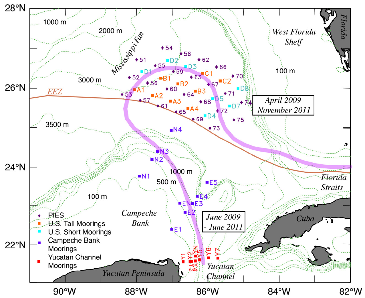
The dataset contains velocity data gathered from June 2009 to June 2011 over the region from $89^{o}W$ to $85^{o}W$, and $25^{o}N$ to $27^{o}N$ with 30–50 $km$ horizontal resolution. Sampling frequency from the multiple sensors varied from minutes to hours. In this study, we utilize a time series which was processed with a fourth order Butterworth filter and sub-sampled at 12-hour intervals. Consequently, the dataset contains a total of 1810 records, covering 905 days. At each time step $t$, the data $\mathcal{X}_{t}$ were formatted as $\mathcal{X}_{t}\subseteq\mathbb{R}^{D\times H\times W\times C}$, where each dimension represents $Depth$ (30), $Longitude$ (29), $Latitude$ (36) and $Channel$ (2), respectively. $Channel$ stands for the geostrophic velocity vector $(u,v)$. The first 80% (June 2009 to December 2010) of the dataset was reserved for training and the remaining 20% (January 2011 to June 2011) for prediction and validation.

Empirical Orthogonal Function (EOF) analysis has been extensively used in the oceanic and atmospheric sciences. In addition to its ability to decompose a time series into its temporal and spatial components, EOF can drastically reduce the dimension while preserving data integrity. Considering the nonlinear dynamics and high dimension characteristics of oceanic phenomena, in this work, the EOF analysis is employed to represent spatial patterns ($EOFs$) and temporal components (Principal Components, $PCs$) of the LCS in the GoM. Specifically, EOF analysis was conducted to extract the $PCs$ of zonal and meridional velocity of ocean current. The $PCs$ may contain otherwise hidden and medium-term uncorrelated patterns (Navarra and Simoncini 2010). Further, $PCs$ are used to train the PITT-ConvLSTM prediction model, with details given in Section 3.

Singular Value Decomposition (SVD) is a general decomposition to determine both the $EOFs$ and $PCs$ simultaneously. For the convenience of ocean modeling, the ocean is sliced into layers in the depth direction. Here, SVD is applied to each depth slice $\mathcal{S}$ to obtain two unitary orthogonal matrices ($U$ and $V$) and one diagonal eigenvalue matrix $\Sigma$. Consequently, $U\Sigma$ represents the temporal $PCs$ and $V^{T}$ the spatial $EOFs$. Thus, $\mathcal{S}$ can be represented as follows,

After the EOF analysis, we concatenate the flattened $PCs$ along the depth dimension. In this way, the raw data $\mathcal{X}\subseteq\mathbb{R}^{T\times D\times H\times W\times C}$ is compressed to ${\mathcal{X}}^{\prime}\subseteq\mathbb{R}^{T\times D\times P\times C}$, where $P$ is the number of selected elements in $PCs$. The 3D volume sequence prediction $\{\mathcal{X}^{(t)}\}_{t=1}^{T}$, in consequence, is compressed to a 2D matrix sequence prediction $\{\mathcal{X}^{\prime(t)}\}_{t=1}^{T}$. Each row of the 2D matrix $\mathcal{X}^{\prime(t)}(i,:)$ (flattened PCs) represents a depth slice of the original 3D volume $\mathcal{X}^{(t)}(i,:,:)$. The model in Section 3 will be trained to predict future $PCs$, which could also be used to reconstruct predicted 3D volume by simply multiplied by the known $EOFs$ (constant) as shown in Equation (1).

Convolutional LSTM network (ConvLSTM), a basic building block for sequence-to-sequence prediction, demonstrated strong performance in video forecasting. In ConvLSTM, the spatial information is encoded explicitly as tensors in the LSTM cells, where each cell is a first-order Markovian model (i.e. the hidden state is updated based on its adjacent step). Since ConvLSTM is successful in modeling complex behaviors and extracting abstract features through real-world data (Xingjian et al. 2015), it is natural to explore how such a predictive model can be used to solve practical problems in physics or engineering domains with higher-order dynamics. In this paper, we propose Physics-informed Tensor-train ConvLSTM (PITT-ConvLSTM), a ConvLSTM network under physics constraints. The ConvLSTM is integrated with convolutional tensor-train to model higher-order spatio-temporal correlations explicitly, with its hidden states incorporated with prior physical knowledge. The proposed model is illustrated in Figure 2 and Figure 3.

ConvLSTM, proposed by (Xingjian et al. 2015) as a convolutional counterpart of conventional FC-LSTM, introduces convolution tensor operation into input-to-state and state-to-state transitions within each recurrent cell. In ConvLSTM, all features are encoded as third-order tensors with dimensions ($Height\times Width\times Channels$). At each time step $t$, a ConvLSTM cell updates its hidden states $\mathcal{H}^{(t)}$ based on the previous $\mathcal{H}^{(t-1)}$ and the current input $\mathcal{X}^{(t)}$:

where $\sigma(\cdot)$ applies sigmoid on the input gate $\mathcal{I}^{(t)}$, forget gate $\mathcal{F}^{(t)}$, and output gate $\mathcal{O}^{(t)}$, and $tanh(\cdot)$ on memory cell $\tilde{\mathcal{C}}^{(t)}$. The $\mathcal{I}^{(t)},\mathcal{F}^{(t)},\mathcal{O}^{(t)},\tilde{\mathcal{C}}^{(t)}\subseteq\mathbb{R}^{H\times W\times C}$, and the parameters are characterized by two 4-$th$ order tensors $\mathcal{W}_{input}\subseteq\mathbb{R}^{K\times K\times S\times 4C}$ and $\mathcal{T}_{hidden}\subseteq\mathbb{R}^{K\times K\times C\times 4C}$, where $K$ is the kernel size, and $S$ and $C$ are the numbers of input channels.

To capture multi-steps spatio-temporal correlations in ConvLSTM, we introduce a higher-order recurrent unit, where the hidden state $\mathcal{H}^{(t)}$ is updated based on the current input $\mathcal{X}^{(t)}$ and its $n$ previous steps $\left\{\mathcal{H}^{(t-l)}\right\}^{n}_{l=1}$ with an $m$-order convolutional tensor-train decomposition $\varphi(\left\{\mathcal{T}^{(l)}\right\}^{m}_{l=1},\cdot)$ as follows:

where the $m$-order convolutional tensor-train $\varphi(\left\{\mathcal{T}^{(l)}\right\}^{m}_{l=1},\cdot)$ are parameterized by $m$ core tensors $\left\{\mathcal{T}^{(l)}\right\}^{m}_{l=1}$. Considering the consistency constraint, the previous $n$ steps are mapped into $m$ intermediate tensors ${\tilde{\mathcal{H}}^{(t,o)}}$ by $f(\mathcal{J},\mathcal{K},\cdot)$ in Equation (3) at first, where $\mathcal{K}$ and $\mathcal{J}$ are 3D convolutional kernels. Note that $f(\mathcal{J},\mathcal{K},\cdot)$ is a mapping function with dynamic physics constraints, which will be discussed in Section 3.3.

The convolutional tensor-train decomposition, first proposed by (Su et al. 2020), is a counterpart of tensor-train decomposition (TTD) which aims to represent a higher-order tensor $\mathcal{T}\subseteq\mathbb{R}^{I_{1}\times\cdots\times I_{m}}$ in a set of smaller and lower-order core tensors $\{\mathcal{T}^{(l)}\}^{m}_{l=1}$ with $\mathcal{T}^{(l)}\subseteq\mathbb{R}^{I_{l}\times R_{l}\times R_{l-1}}$. The ranks $\{R^{(l)}\}^{m}_{l=1}$ here control the number of parameters in the tensor-train format. In this way, the original $\mathcal{T}$ of size $\prod_{l=1}^{m}I_{l}$ is compressed to $\sum_{l=1}^{m}I_{l}R_{l-1}R_{l}$, i.e. the complexity only grows linearly with the order $m$ (assuming $R_{l}$’s are constants). Similar to TTD, $\varphi$ is designed to significantly reduce both parameters and operations of higher-order spatio-temporal recurrent models by factorizing a large convolutional kernel into a chain of smaller kernels. The details of convolutional tensor-train decomposition $\mathcal{T}=\mathcal{CTTD}\left\{\mathcal{T}^{(l)}\right\}^{m}_{l=1}$ is formulated as:

and the convolutional tensor-train for spatial-temporal modeling can be equivalently stated as:

where $\mathcal{U}$ is the input feature corresponding to $\tilde{\mathcal{H}}$. $\left\{\mathcal{V}^{l}\right\}_{l=1}^{m}$ are intermediate results, in which $\mathcal{V}^{l}\subseteq\mathbb{R}^{H\times W\times R_{l}}$ for $l>1$, and $\mathcal{V}^{1}\subseteq\mathbb{R}^{H\times W\times R_{m}}$ is initialized as all zeros and final prediction is returned as $\mathcal{V}=\mathcal{V}^{m+1}$. The exact mathematical proof is included in Appendix A.

In this section, we provide how the law of physics that describes the physical processes (e.g., the LCS) can be incorporated into the deep learning framework. Physical processes are often modeled by a set of nonlinear partial differential equations (PDEs), which describe how a physical quantity is changed in a given region over time. Such dynamic equations are usually written as a relation between time derivatives and spatial derivatives:

where $u$ is a physical quantity, say, velocity, and $x$ is its spatial coordinate. Furthermore, coefficients $b_{i}$, $c_{i}$ are functions of $u$ and $x$. Finally, $P$ and $Q$ denote the highest order of time derivatives and spatial derivatives, respectively.

There are multiple ways to incorporate the physical laws into neural networks. In this paper, inspired by (Seo and Liu 2019), we model the law of physics by replacing the updating functions in neural networks with corresponding operators. Considering the characteristics of ocean current, we adopt two dynamic equations, i.e. the diffusion equation and the wave equation, shown in Table 1. The diffusion equation describes the behavior of the continuous physical quantities (macroscopic behavior of many micro-particles in Brownian motion) resulting from the random movement. The wave equation is a second-order PDE for the description of waves (e.g. water, sound, or seismic waves).

In Equation (3), a sliding window strategy is adopted. As shown in Figure 2, a sliding subset of $\{\mathcal{H}^{l}\}$ are concatenated and then transformed into $m$ (i.e. the number of core tensors in $\varphi$) intermediate hidden tensor $\{\mathcal{H}^{(t,o)}\}$. The concrete process is as follows:

where $n$ is the sliding window size. The $\{\mathcal{H}\}^{n}_{l=1}$ are first concatenated into $m$ tensors $\{\mathcal{H}_{cat}\}^{m}_{l=1}$ ($\mathcal{H}_{cat}\subseteq\mathbb{R}^{H\times W\times(n-m+1)\times C}$) along the time axis, which are thereafter mapped to $\mathcal{H}^{(t,o)}\subseteq\mathbb{R}^{H\times W\times R}$ by the 3D convolutional kernel $\mathcal{K}^{o}\subseteq\mathbb{R}^{K\times K\times(n-m+1)\times R}$.

Then, we update the intermediate hidden tensor $\{\mathcal{H}^{(t,o)}\}$ to $\{\tilde{\mathcal{H}}^{(t,o)}\}$ with physics constraints (see Pseudocode in Appendix B). Finally, the sequentially updated intermediate hidden tensor are transformed to the output space by convolutional tensor-train decomposition described in Section 3.2. It is notable that the law of physics is not directly constrained to the raw observations, but rather to the latent representations (i.e. the hidden states of ConvLSTM in this work). This is a desired configuration considering the difficulty in identifying which observations are following the law of physics explicitly and how much in accordance. Consequently, instead of individually applying the equation to each observation, we found that it is more efficient to introduce the constraints on the latent representations.

As illustrated in Figure 2, $\mathcal{J}$ is the learn-able parameter vector while the orange blocks (“Physics Equation”) are objective functions related to physics constraints. First, we define physics constraints between the previous and updated states based on the known/assumed knowledge as:

where $\emph{g}$ is case-specific. In particular, if we are aware/assume that the observations should have a diffusive property, the diffusion equation can be used as the physics-informed constraint as:

where $v$ (or ${v}^{\prime}$) is the corresponding element of $\mathcal{H}$ (or $\tilde{\mathcal{H}}$).

The physics-informed objective function of the total sequence is defined as:

and the overall objective function is the sum of the supervised loss and physical loss:

where $\mathcal{L}_{1}$ is the mean absolute error, $\mathcal{L}_{2}$ is the mean squared error, and $\lambda$ controls the importance of physics term.

Model-based LC prediction primarily uses finite-differences or finite-element techniques to discretize PDEs in numerical models. The classical Princeton Regional Ocean Forecast System (Oey et al. 2005) used data assimilation techniques to constrain their model solution with remote and in situ observations. Later, a local ensemble transform Kalman filter was applied to Princeton Ocean Model (Xu et al. 2013) to estimate sea surface heights and LC temperatures. An ensemble based optimal interpolation technique (Counillon and Bertino 2009) was further used to assimilate altimetry in the Hybrid Coordinate Ocean Model to predict LC eddy shedding. In the GoM 3-D Operational Ocean Forecast System Pilot Prediction Project (Mooers et al. 2012), several mesoscale eddy-resolving baroclinic ocean circulation numerical models were evaluated. With the popularization of machine learning, (Zeng et al. 2015) proposed a novel model based on artificial neural network and EOF analysis for the LCS evolution prediction. Recently, a Divide-and-Conquer prediction model based on the LSTM network was developed to forecast the evolution of the LC and its eddy shedding (Wang et al. 2019). It was capable of predicting the LC evolution for a period of 9 weeks, and the timing and general location of eddy Darwin’s shedding event 12 weeks in advance, and eddy Cameron’s detachment and reattachment 8 weeks in advance.

TTD, as a principled approach that factorizes the model parameters into smaller tensors (Oseledets 2011) for addressing the curse of dimensionality, is especially beneficial in multi-relational data analysis, and has been widely used in machine learning, including CNNs (Kolbeinsson et al. 2019; Su et al. 2018; Su et al. 2020), RNNs (Yang et al. 2017; Su et al. 2020) and transformers (Ma et al. 2019). A multiplicative RNNs with factorized weights tensor was proposed for inputs-states interactions (Sutskever et al. 2011). Further, (Yang et al. 2017) factorized the input-to-hidden weights within each cell by TTD, and showed improvement in video classification. Different from the first-order RNNs mentioned above, higher-order RNNs (Soltani and Jiang 2016) require excessively more parameters since they introduce connections cross multiple previous time steps for better long-term dynamics learning. This was improved by TT-RNNs (Yu et al. 2018), whose higher-order structures within each cell were compressed by TTD while improving the model performance in video classification. Recently, (Su et al. 2020) introduced a novel convolutional TTD and constructed Convolutional Tensor-Train LSTM to capture higher-order space-time correlations.

Physics is one of the fundamental pillars explaining how nature behaves. Concerning that it is unable to describe all rules governing real-world data, machine learning is desired to bridge the known physics and observations. (Raissi et al. 2017; Raissi and Karniadakis 2018; Raissi 2018) demonstrate that neural networks are capable of finding solutions to PDEs, which enables us to obtain fully differentiable physics-informed models with respect to all input coordinates and free parameters. (de Bezenac et al. 2019) demonstrates how fluid physics could be incorporated for forecasting sea surface temperature, and such method not only captures the dominant physics but also infers unknown patterns by CNNs. Further, growing physics-informed models (Sanchez-Gonzalez et al. 2018; Kipf et al. 2018) were developed, assuming that neural networks can learn complex dynamic interactions and simulate unseen dynamics based on a current state. Unlike those works that implicitly extracts latent patterns from data only, the physics-informed Graph networks proposed in (Seo and Liu 2019) allow incorporating known physics and simultaneously extracting latent patterns in data which is unable to be captured by existing knowledge.

References

- Bengio et al. [2015] Samy Bengio, Oriol Vinyals, Navdeep Jaitly, and Noam Shazeer. Scheduled sampling for sequence prediction with recurrent neural networks. In Advances in Neural Information Processing Systems, pages 1171–1179, 2015.
- Byeon et al. [2018] Wonmin Byeon, Qin Wang, Rupesh Kumar Srivastava, and Petros Koumoutsakos. Contextvp: Fully context-aware video prediction. In Proceedings of the European Conference on Computer Vision (ECCV), pages 753–769, 2018.
- Counillon and Bertino [2009] François Counillon and Laurent Bertino. High-resolution ensemble forecasting for the gulf of mexico eddies and fronts. Ocean Dynamics, 59(1):83–95, 2009.
- de Bezenac et al. [2019] Emmanuel de Bezenac, Arthur Pajot, and Patrick Gallinari. Deep learning for physical processes: Incorporating prior scientific knowledge. Journal of Statistical Mechanics: Theory and Experiment, 2019(12):124009, 2019.
- Donohue et al. [2016] Kathleen A Donohue, DR Watts, P Hamilton, R Leben, and M Kennelly. Loop current eddy formation and baroclinic instability. Dynamics of Atmospheres and Oceans, 76:195–216, 2016.
- Hamilton et al. [2016] Peter Hamilton, Alexis Lugo-Fernández, and Julio Sheinbaum. A loop current experiment: Field and remote measurements. Dynamics of Atmospheres and Oceans, 76:156–173, 2016.
- Kingma and Ba [2014] Diederik P Kingma and Jimmy Ba. Adam: A method for stochastic optimization. arXiv preprint arXiv:1412.6980, 2014.
- Kipf et al. [2018] Thomas Kipf, Ethan Fetaya, Kuan-Chieh Wang, Max Welling, and Richard Zemel. Neural relational inference for interacting systems. arXiv preprint arXiv:1802.04687, 2018.
- Kolbeinsson et al. [2019] Arinbjörn Kolbeinsson, Jean Kossaifi, Yannis Panagakis, Adrian Bulat, Anima Anandkumar, Ioanna Tzoulaki, and Paul Matthews. Robust deep networks with randomized tensor regression layers. arXiv preprint arXiv:1902.10758, 2019.
- Ma et al. [2019] Xindian Ma, Peng Zhang, Shuai Zhang, Nan Duan, Yuexian Hou, Ming Zhou, and Dawei Song. A tensorized transformer for language modeling. In Advances in Neural Information Processing Systems, pages 2229–2239, 2019.
- Mooers et al. [2012] CNK Mooers, ED Zaron, and MK Howard. Final report for phase i: Gulf of mexico 3-d operational ocean forecast system pilot prediction project (gomex-ppp). Final Rep. to Research Partnership to Secure Energy for America, 2012.
- NAS et al. [2018] NAS et al. Understanding and predicting the gulf of mexico loop current: Critical gaps and recommendations. National Academies Press, 2018.
- Navarra and Simoncini [2010] Antonio Navarra and Valeria Simoncini. A guide to empirical orthogonal functions for climate data analysis. Springer Science & Business Media, 2010.
- Oey et al. [2005] L-Y Oey, Tal Ezer, George Forristall, C Cooper, Steven DiMarco, and S Fan. An exercise in forecasting loop current and eddy frontal positions in the gulf of mexico. Geophysical Research Letters, 32(12), 2005.
- on the BP Deepwater Horizon Spill et al. [2011] National Commission on the BP Deepwater Horizon Spill, Offshore Drilling (US), Bob Graham, and William Kane Reilly. Deep water: the gulf oil disaster and the future of offshore drilling: report to the president. The Commission, 2011.
- Oseledets [2011] Ivan V Oseledets. Tensor-train decomposition. SIAM Journal on Scientific Computing, 33(5):2295–2317, 2011.
- Raissi [2018] Maziar Raissi. Deep hidden physics models: Deep learning of nonlinear partial differential equations. The Journal of Machine Learning Research, 19(1):932–955, 2018.
- Raissi and Karniadakis [2018] Maziar Raissi and George Em Karniadakis. Hidden physics models: Machine learning of nonlinear partial differential equations. Journal of Computational Physics, 357:125–141, 2018.
- Raissi et al. [2017] Maziar Raissi, Paris Perdikaris, and George Em Karniadakis. Physics informed deep learning (part i): Data-driven solutions of nonlinear partial differential equations. arXiv preprint arXiv:1711.10561, 2017.
- Sanchez-Gonzalez et al. [2018] Alvaro Sanchez-Gonzalez, Nicolas Heess, Jost Tobias Springenberg, Josh Merel, Martin Riedmiller, Raia Hadsell, and Peter Battaglia. Graph networks as learnable physics engines for inference and control. arXiv preprint arXiv:1806.01242, 2018.
- Seo and Liu [2019] Sungyong Seo and Yan Liu. Differentiable physics-informed graph networks. arXiv preprint arXiv:1902.02950, 2019.
- Soltani and Jiang [2016] Rohollah Soltani and Hui Jiang. Higher order recurrent neural networks. arXiv preprint arXiv:1605.00064, 2016.
- Su et al. [2018] Jiahao Su, Jingling Li, Bobby Bhattacharjee, and Furong Huang. Tensorized spectrum preserving compression for neural networks. arXiv preprint arXiv:1805.10352, 2018.
- Su et al. [2020] Jiahao Su, Wonmin Byeon, Furong Huang, Jan Kautz, and Animashree Anandkumar. Convolutional tensor-train lstm for spatio-temporal learning. arXiv preprint arXiv:2002.09131, 2020.
- Sutskever et al. [2011] Ilya Sutskever, James Martens, and Geoffrey E Hinton. Generating text with recurrent neural networks. In Proceedings of the 28th international conference on machine learning (ICML-11), pages 1017–1024, 2011.
- Walker et al. [2009] Nan Walker, Robert Leben, Steve Anderson, Jim Feeney, Patrice Coholan, and Neha Sharma. Loop current frontal eddies based on satellite remote-sensing and drifter data. 2009.
- Wang et al. [2019] Justin L Wang, Hanqi Zhuang, Laurent M Chérubin, Ali K Ibrahim, and Ali Muhamed Ali. Medium-term forecasting of loop current eddy cameron and eddy darwin formation in the gulf of mexico with a divide-and-conquer machine learning approach. Journal of Geophysical Research: Oceans, 124(8):5586–5606, 2019.
- Wang et al. [2017] Yunbo Wang, Mingsheng Long, Jianmin Wang, Zhifeng Gao, and S Yu Philip. Predrnn: Recurrent neural networks for predictive learning using spatiotemporal lstms. In Advances in Neural Information Processing Systems, pages 879–888, 2017.
- Wang et al. [2004] Zhou Wang, Alan C Bovik, Hamid R Sheikh, and Eero P Simoncelli. Image quality assessment: from error visibility to structural similarity. IEEE transactions on image processing, 13(4):600–612, 2004.
- Xingjian et al. [2015] SHI Xingjian, Zhourong Chen, Hao Wang, Dit-Yan Yeung, Wai-Kin Wong, and Wang-chun Woo. Convolutional lstm network: A machine learning approach for precipitation nowcasting. In Advances in neural information processing systems, pages 802–810, 2015.
- Xu et al. [2013] F-H Xu, L-Y Oey, Y Miyazawa, and P Hamilton. Hindcasts and forecasts of loop current and eddies in the gulf of mexico using local ensemble transform kalman filter and optimum-interpolation assimilation schemes. Ocean Modelling, 69:22–38, 2013.
- Yang et al. [2017] Yinchong Yang, Denis Krompass, and Volker Tresp. Tensor-train recurrent neural networks for video classification. In Proceedings of the 34th International Conference on Machine Learning-Volume 70, pages 3891–3900. JMLR. org, 2017.
- Yu et al. [2018] Rose Yu, Stephan Zheng, Anima Anandkumar, and Yisong Yue. Long-term forecasting using tensor-train rnns. h ps. In openreview. net/forum, 2018.
- Zeng et al. [2015] Xiangming Zeng, Yizhen Li, and Ruoying He. Predictability of the loop current variation and eddy shedding process in the gulf of mexico using an artificial neural network approach. Journal of Atmospheric and Oceanic Technology, 32(5):1098–1111, 2015.