Risk-sensitive Dynkin games with heterogeneous Poisson random intervention times Thanks: We thank David Hobson for the suggestion of considering heterogenous signal times for constrained Dynkin games, which motivates the current project.

Risk-sensitive criteria constitute a genuinely interesting class of performance criteria in optimization problems, in which the linear expectation $\mathbb{E}[\cdot]$ is replaced by the nonlinear expectation

for some strictly increasing function $g$ as a risk-sensitive function. The corresponding risk-sensitive control has been developed to reflect an optimizer’s attitudes to risks. In particular, the risk-sensitive function $g$ is chosen to model the optimizer’s attitudes towards risks (e.g. strict concavity of $g$ reflects risk-aversion of maximization players or risk-seeking of minimization players).

In this paper, we are interested in Dynkin games with risk-sensitive criteria, by taking into account of both players’ attitudes to risks. Namely, the two players aim to minimize/maximize some payoff functional $R(\sigma,\tau)$ under the nonlinear expectation $\tilde{\mathbbm{E}}[\cdot]$:

where $\sigma$ and $\tau$ are the stopping times to be chosen by the respective minimization/maximization players. It is called risk-sensitive because

where $l_{g}(x)=-\frac{g^{\prime\prime}(x)}{g^{\prime}(x)}$ is the Arrow-Pratt function of absolute risk aversion. The case $g(x)=x$ corresponds to a risk-neutral attitude of both players since $l_{g}(x)=0$. For the case of an exponential utility $g(x)=-e^{-\gamma x}$ with $\gamma>0$, $l_{g}(x)=\gamma$ is constant and the risk-sensitivity is only expressed through the risk-sensitivity parameter $\gamma$.

The stopping time strategies of the two players are restricted to two independent sequences of Poisson arrival times as the exogenous constraints on the players’ abilities to stop. The constraints may represent liquidity effects, indicating the times at which the underlying stochastic processes are available to stop. Applications of such a liquidity model can be found in [24] for bank runs and [25] for convertible bonds. The constraints can also be seen as information constraints. The players are allowed to make their stopping decisions at all times, but they are only able to observe the underlying stochastic processes at Poisson arrival times. See [11] and [21] for applications to perpetual American options. Due to the introduction of constraints on stopping times and risk-sensitive criteria, we call the Dynkin games considered in this paper the constrained risk-sensitive Dynkin games.

We generalize our previous work [25] on constrained Dynkin games in two aspects: First, it takes into consideration of both players’ attitudes towards risks via the risk-sensitive function $g$; Second, there are control constraints for both players and, moreover, the constraints are different in the sense that they are allowed to stop at two heterogeneous sequences of Poisson arrival times. Consequently, since the two players’ stopping time strategies are chosen from two different sequences of signal times, the usual condition of the upper obstacle $U$ dominating the lower one $L$ is not required. In [25], the risk-sensitive function $g(x)=x$ and both players stop at a single sequence of signal times (so $U\geq L$ is assumed therein).

New challenges arise from the above generalizations. Since the two players stop at two different sequences of Poisson arrival times, the first step to solve the constrained risk-sensitive Dynkin game is merging the two Poisson sequences together while still keeping track of their order. This is crucial when we consider a family of constrained risk-sensitive Dynkin games (3.5)-(3.6) starting from different signal times in order to apply the dynamic programming principle. Note that the starting times of the games (3.5)-(3.6) may not be the respective player’s own Poisson signal times; instead they could be from the counterparty’s signal times. To deal with the nonlinear expectation $\tilde{\mathbbm{E}}$ arising from the risk-sensitive function $g$, we introduce a new transformation resulting the auxiliary payoff processes (2.7)-(2.9), which enable us to rewrite the payoff functional under the linear expectation $\mathbb{E}$ instead of the nonlinear expectation $\tilde{\mathbbm{E}}$. For a special case of exponential risk-sensitive function $g$ (see section 5.2), the representation formula (2.10) of the game value is closely related to Cole-Hopf transformation in the literature of backward stochastic differential equations (BSDEs for short), which is widely used to linearize a class of BSDEs with quadratic growth (see [18]). Our representation formula (2.10) can be regarded as a stochastic control version of Cole-Hopf transformation.

We also make a connection of constrained risk-sensitive Dynkin games with a class of stochastic differential games via Krylov’s randomized stopping technique (see [19]). It is established in [19] that standard optimal stopping problems (without constraints on stopping times) admit stochastic control representation, which can be further solved via the so-called normalized Bellman equations. The stochastic control representation of the corresponding constrained optimal stopping problems has been established in [23] (see section 4 therein). In a constrained stopping game setting as considered in the current paper, it is natural to expect that a stochastic differential game representation should hold accordingly. Indeed, we show that the two players in the stochastic differential game choose their respective running controls and discount rates with binary values $0$ or the Poisson intensity $\lambda^{i}$, and the optimal control is the Poisson intensity $\lambda^{i}$ whenever the value of the game falls below the lower obstacle process/goes above the upper obstacle process.

Turing to the literature of Dynkin games, there has been a considerable development since the seminal works of Dynkin [12] and Neveu [32]. The continuous time models were developed, among others, by Bismut [5], Alario-Nazaret et al [1], Lepeltier and Maingueneau [22] and Morimoto [30]. In order to relax the dominating condition $U\geq L$ in those papers, Yasuda [36] proposed the strategies of randomized stopping times, and proved that the game value exists under merely an integrability condition. Rosemberg et al [34], Touzi and Vielle [35] and Laraki and Solan [20] further extended his work in this direction. The non-Markovian case was addressed in Cvitanic and Karatzas [7] for a fixed horizon and Hamadene et al [14] for an infinite horizon using the theory of reflected BSDEs. If the two players in the game are with asymmetric payoffs/information, then it gives arise to a nonzero-sum Dynkin game. See, for example, Hamadene and Zhang [15], De Angelis et al [10] and, more recently, De Angelis and Ekstrom [9] with more references therein. A robust version of Dynkin games can be found in Bayraktar and Yao [4] if the players are ambiguous about their probability model.

On the other hand, the risk-sensitive optimal stopping problems have been studied by Nagai [31], Bäuerle and Rieder [3], Bäuerle and Popp [2] and, more recently, Jelito et al [17]. For the risk-sensitive zero-sum and nonzero-sum stochastic differential games, we refer to El-Karoui and Hamadène [13]. To the best of our knowledge, the study of risk-sensitive Dynkin games is still lacking, no matter with or without constraints on stopping time strategies. The current paper offers a first step to understand risk-sensitive Dynkin games, in particular with constraints on the stopping time strategies.

The constrained optimal stopping problems was first studied by Dupuis and Wang [11], where they used it to model perpetual American options exercised at exogenous Poisson arrival times. See also Lempa [21], Menaldi and Robin [27] and Hobson and Zeng [16] for further extensions of this type of optimal stopping models. From a different perspective, Liang [23] made a connection between such kind of optimal stopping problems with penalized BSDEs. The corresponding optimal switching (impulse control) models were studied by Liang and Wei [26], and by Menaldi and Robin [28] [29] with more general signal times and state spaces. More recently, Liang and Sun [25] introduced the corresponding constrained Dynkin games (with the risk-sensitive function $g(x)=x$), where both players were allowed to stop at a sequence of random times generated by a single exogenous Poisson process serving as a signal process.

The paper is organized as follows. Section 2 contains the problem formulation and main result, with its proof provided in section 3. In section 4, we establish its connection with a class of stochastic differential games, and in section 5 we further provide two examples. Finally, section 6 concludes the paper.

Let $(\Omega,\mathcal{F},\mathbbm{P})$ be a complete probability space endowed with a $d$-dimensional standard Brownian motion $(W_{t})_{t\geq 0}$ with $\mathbbm{F}=\{\mathcal{F}_{t}\}_{t\geq 0}$ being the minimal augmented filtration of $W$. The probability space also supports two independent sequences of Poisson arrival times $T^{(1)}=\{T^{(1)}_{n}\}_{n\geq 0}$ and $T^{(2)}=\{T^{(2)}_{n}\}_{n\geq 0}$ with their respective intensities $\lambda^{(1)}$ and $\lambda^{(2)}$ and the minimal augmented filtration $\mathbbm{H}=\{\mathcal{H}_{t}\}_{t\geq 0}$, satisfying $T^{(1)}_{0}=T^{(2)}_{0}=0$ and $T^{(1)}_{\infty}=T^{(2)}_{\infty}=\infty$. Denote the smallest filtration generated by $\mathbbm{F}$ and $\mathbbm{H}$ as $\mathbbm{G}=\{\mathcal{G}_{t}\}_{t\geq 0}$, i.e. $\mathcal{G}_{t}=\mathcal{F}_{t}\vee\mathcal{H}_{t}$, and write $\bm{\lambda}=(\lambda^{(1)},\lambda^{(2)})$.

Let $T$ be a finite $\mathbbm{F}$-stopping time representing the (random) terminal time of the game. For each player $i\in\{1,2\}$, let us define a random variable $M_{i}:\Omega\mapsto\mathbbm{N}$ such that $T_{M_{i}}$ is the next arrival time in the Poisson sequence $T^{(i)}$ following $T$, i.e. $M_{i}(\omega):=\sum_{n\geq 1}n\mathbbm{1}_{\{T^{i}_{n-1}(\omega)\leq T(\omega)<T^{i}_{n}(\omega)\}}$.

For any integer $n\geq 0$, let us define the control set for each player $i\in\{1,2\}$ as

so the player $i$ chooses from the Poisson arrival times $T^{(i)}$ with intensity $\lambda^{(i)}$, and $T_{n}^{(i)}$ is the smallest stopping time allowed.

Consider a constrained risk-sensitive Dynkin game, where the two players choose their respective stopping times $\sigma\in\mathcal{R}_{1}^{(1)}$ and $\tau\in\mathcal{R}_{1}^{(2)}$ in order to minimize/maximize the expected cost functional

where the nonlinear expectation $\tilde{\mathbbm{E}}:\mathbbm{R}\to\mathbbm{R}$ is defined via the risk-sensitive function $g$, i.e.

The discounted payoff functional $R(\sigma,\tau)$ in (2.2) is defined by

where $r>0$ is the discount rate, and $f$, as a real-valued $\mathbbm{F}$-progressively measurable process, is the running payoff. The terminal payoff is $U$ if $\sigma$ happens firstly, $L$ if $\tau$ happens firstly or $\sigma$ and $\tau$ happen simultaneously, and $\xi$ otherwise, where $L$ and $U$ are two real-valued $\mathbbm{F}$-progressively measurable processes, and $\xi$ is a real-valued $\mathcal{F}_{T}$-measurable random variable.

Let us define the upper and lower values of the constrained risk-sensitve Dynkin game

The game (2.5) is said to have value $v^{\bm{\lambda}}$ if $v^{\bm{\lambda}}=\overline{v}^{\bm{\lambda}}=\underline{v}^{\bm{\lambda}}$, and a saddle point $(\sigma^{*},\tau^{*})\in\mathcal{R}_{1}^{(1)}\times\mathcal{R}_{1}^{(2)}$ is called an optimal stopping strategy of the game if

for every $(\sigma,\tau)\in\mathcal{R}_{1}^{(1)}\times\mathcal{R}_{1}^{(2)}$.

Compared with the constrained Dynkin game introduced in [25], there are two new features of the game (2.5): First, it takes into consideration of the both players’ attitudes towards risks via the risk-sensitive function $g$; Second, there are control constraints for both players and, moreover, the constraints are different in the sense that they are allowed to stop at two heterogeneous sequences of Poisson arrival times. As a consequence, since the two players’ stopping time strategies are chosen from two different control sets, the usual dominating condition $U\geq L$ is not required. In [25], the risk-sensitive function $g(x)=x$ and both players stop at a single sequence of Poisson arrival times (so $U\geq L$ is a critical assumption therein).

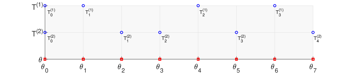
Since the two players stop at two different sequences of Poisson arrival times, the first step to prove Theorem 2.3 is merging the two Poisson sequences together while still keeping track of their order. To this end, for each $T^{(1)}$ and $T^{(2)}$, we construct an increasing sequence of $\mathbbm{G}$-stopping times $\theta=(\theta_{k})_{k\geq 0}$ as follows:

In Figure 1, we illustrate the construction of the merged sequence $\theta$, where the top and the middle line are a realization of $T^{(1)}$ and $T^{(2)}$, and the bottom line is the merged sequence $\theta$. Intuitively, given any $\mathbbm{G}$-stopping time $\theta_{k-1}$, $k\geq 1$, (to be used as the starting times for a family of constrained Dynkin games (3.5)-(3.6) below), we find the first arrival time of each Poisson sequence following $\theta_{k-1}$, say $T^{(1)}_{k_{1}}$ and $T^{(2)}_{k_{2}}$ for some $k_{1},k_{2}\geq 0$, and then define $\theta_{k}=\min\{T^{(1)}_{k_{1}},T^{(2)}_{k_{2}}\}$. Moreover, given the stopping time $\theta_{k}$, we define pre-$\theta_{k}$ $\sigma$-field:

and $\tilde{\mathbbm{G}}=\{\mathcal{G}_{\theta_{k}}\}_{k\geq 0}$.

Next, we tackle the nonlinear expectation $\tilde{\mathbbm{E}}$ associated with the risk-sensitive function $g$. To this end, introduce the discounted processes

and rewrite the discounted payoff functional $R(\sigma,\tau)$ as

In turn, consider a family of constrained risk-sensitive Dynkin games starting from $\theta_{k-1}$, for $k\geq 1$, whose upper and lower values are defined by

where

The constrained risk-sensitive Dynkin game (3.5)-(3.6) is said to have value $q_{\theta_{k-1}}^{\bm{\lambda}}$ if $q_{\theta_{k-1}}^{\bm{\lambda}}=\overline{q}_{\theta_{k-1}}^{\bm{\lambda}}=\underline{q}_{\theta_{k-1}}^{\bm{\lambda}}$, and $(\sigma^{*}_{k},\tau^{*}_{k})\in\tilde{\mathcal{R}}^{(1)}_{\theta_{k}}\times\tilde{\mathcal{R}}^{(2)}_{\theta_{k}}$ is called an optimal stopping strategy of the game if

for every $(\sigma,\tau)\in\tilde{\mathcal{R}}^{(1)}_{\theta_{k}}\times\tilde{\mathcal{R}}^{(2)}_{\theta_{k}}$. In particular, when $k=1$, (3.5)-(3.6) corresponds to the original constrained Dynkin game (2.5). Thus, to prove Theorem 2.3, it is sufficient to show that

and the optimal stopping strategy is given by

where $\tilde{Q}^{\bm{\lambda}}$ is given by

with $\overline{Q}^{\bm{\lambda}}$ being the first component of the solution to BSDE (2.6). In turn, the value process $Q^{\bm{\lambda}}$ in (2.3) is given via the discounted process $\tilde{Q}^{\bm{\lambda}}$ via the relationship

Note that, for $t\geq T$,

To prove the above assertions (and therefore Theorem 2.3), we start with the following lemma.

Proof. It is equivalent to prove that

where $g(\tilde{\xi})=e^{-rT}\overline{\xi}$, $g(\tilde{L}_{t})=e^{-rt}\overline{L}_{t}$ and $g(\tilde{U}_{t})=e^{-rt}\overline{U}_{t}$. For $k$ such that $\theta_{k-1}>T$, it follows from (3.9) that $g(\tilde{Q}_{\theta_{k-1}}^{\bm{\lambda}})=g(\tilde{\xi})$, and thus (3.12) holds. In the rest of the proof, we only focus on the cases where $\theta_{k-1}\leq T$.

By applying Itô’s formula to $\alpha_{t}g(\tilde{Q}_{t}^{\bm{\lambda}})$, where $\alpha_{t}=e^{-(\lambda^{(1)}+\lambda^{(2)})t}$, we can obtain that

for $t\geq 0$. By choosing $t=\theta_{k-1}$ and taking the conditional expectation with respect to $\mathcal{G}_{\theta_{k-1}}$, we further have

for any $k\geq 1$.

On the other hand, by defining $\tilde{T}^{(i)}_{t}$ as the first arrival time in $T^{(i)}$ following any fixed time $t$, i.e. $\tilde{T}^{(i)}_{t}=\inf\{T_{N}^{(i)}\geq T_{1}^{(i)}:T_{N}^{(i)}>t\}$, we can rewrite the right-hand-side of (3.12) as

Indeed, applying the joint probability density function of $(\tilde{T}^{(1)}_{\theta_{k-1}},\tilde{T}^{(2)}_{\theta_{k-1}})$ conditional on $\mathcal{G}_{\theta_{k-1}}$,

yields that

where the first integral