Revealing the Local Cosmic Web from Galaxies by Deep Learning HEALPix (Górski et al. 2005), Healpy (Zonca et al. 2019), astropy (Astropy Collaboration et al. 2013; Astropy Collaboration et al. 2018), NumPy (Van Der Walt et al. 2011; Harris et al. 2020), Scipy (Jones et al. 2001; Virtanen et al. 2020), matplotlib (Hunter 2007), pandas (Wes McKinney 2010), Keras (Chollet et al. 2015), Tensorflow backend (Abadi et al. 2015)

We use the Cosmicflows-3 galaxy catalog (Tully et al. 2016, CF3 hereafter), one of the most comprehensive galaxy catalogs that provide distance, radial peculiar velocity, and luminosity of 17,647 galaxies up to $200~{\rm Mpc}$. To produce a fair galaxy sample over the given region, we make the volume-limited sub-sample of the CF3 as follows. First, as the number density of the CF3 galaxies close to the Galactic plane (Galactic latitude $|b|<10^{\circ}$) is lower than average, we only use the galaxies at $|b|>10^{\circ}$. Also, we use the $B$-band absolute magnitude ($M_{B}$) compiled from Lyon Extragalactic Database (Paturel et al. 2003, LEDA;) as a proxy of the stellar mass (Wilman & Erwin 2012, $M_{\star}$;). We set the $B$-band magnitude $-15$ as the selection criterion, which is sufficient for covering the $20\mathinner{{\rm Mpc}/h}$- and $40\mathinner{{\rm Mpc}/h}$-cubic volume around the Milky-way galaxy. We have also tested the cases with $M_{B}<-16$ and $-17$ and found no noticeable difference of the predictions from the fiducial choice (see Section IV). Note that we have not used the $K_{S}$-band absolute magnitude, one of the best-known tracers of the stellar mass (Bell et al. 2003) because that information is missing for about 30% of the galaxies in our sample (Lavaux & Hudson 2011; Huchra et al. 2012).

We calculate the radial peculiar velocity by subtracting the Hubble flow from the velocity in the Galactic Standard of Rest (Kourkchi et al. 2020, $V_{\rm GSR}$;). Note that we do not use the velocity in the cosmic microwave background (CMB) standard of rest ($V_{\rm CMB}$)to reduce any bias that might be introduced in the conversion. Instead, when generating training and test samples from simulation data, we include the peculiar motion of the Milky-way corresponding galaxy in each simulation. There exists a difference on the Hubble constant between recent CMB observations (Planck Collaboration et al. 2018, $H_{0}=67.77\,{\rm km/s/Mpc}$;) and the best-fit from the CF3 (Tully et al. 2016, $H_{0}=75\,{\rm km/s/Mpc}$;). In this study, we have tested both values and find that the effect from the different Hubble constants stays within the uncertainty of the dark-matter map (see Section IV).

We use the TNG100-1, a simulation with a comoving volume $V=(75\mathinner{{\rm Mpc}/h})^{3}$ and $1820^{3}$ dark-matter and gas particles from the Illustris-TNG simulation suite (Springel et al. 2018; Pillepich et al. 2018; Marinacci et al. 2018; Naiman et al. 2018; Nelson et al. 2018; Nelson et al. 2019), as our high-resolution simulation data (TNG100 hereafter). To mimic the observation from the Milky-way galaxy, we select 988 galaxies with stellar mass $4\times 10^{10}\mathinner{{\rm M}_{\odot}}<M_{\star}<10^{11}\mathinner{{\rm M}_{\odot}}$ (center galaxies hereafter)by adopting that the Galactic stellar mass is about $5.2\times 10^{10}\mathinner{{\rm M}_{\odot}}$ (Licquia & Newman 2015). Around each center galaxy, we make a sub-cube with $20\mathinner{{\rm Mpc}/h}$ box-size and calculate the dark-matter density field within the $64^{3}$ uniform grid. We also calculate the relative position of galaxies with $M_{B}<-15$ (target galaxies hereafter) and the difference of peculiar velocity between the target galaxy and center galaxy.

For the low-resolution dark-matter map with $V=(40\mathinner{{\rm Mpc}/h})^{3}$, we use the TNG300-1 from the Illustris-TNG simulations, whose volume and number of particles are $V=(205\mathinner{{\rm Mpc}/h})^{3}$ and $2500^{3}$, respectively (TNG300 hereafter). Note that the amplitude of the luminosity function of TNG300 is lower than the observation and TNG100, mainly due to the lower spatial resolution of the simulation (Pillepich et al. 2018). Therefore, we also apply the resolution correction to find the center and target galaxies using the number density obtained from TNG100 rather than directly using the face values of $M_{\star}$ or $M_{B}$. We also use the TNG300-1-Dark, a dark-matter-only counterpart of the TNG300, to test how baryonic physics affects our result. We select the center and target galaxies by finding the mass cut of dark matter halos with the same number density. The result from the TNG300-1-Dark is similar to or slightly worse than TNG300 (see Section IV).

Also, we use the RefL0100N1504, a reference simulation with $V=(67.77\mathinner{{\rm Mpc}/h})^{3}$ and $1504^{3}$ dark-matter and gas particles from the EAGLE simulation suite (Schaye et al. 2015; Crain et al. 2015, EAGLE hereafter), to check the fidelity of our result. For the center galaxies, we use the same selection criterion to TNG100 and find 478 center galaxies. For the target galaxies, however, we do not directly use $M_{B}$. It is because the luminosity function of EAGLE is reliable only for bright galaxies ($M_{B}\lesssim-18$) since the EAGLE simulations calculate the luminosity only to massive galaxies (Camps et al. 2018, $M_{\star}\geq 10^{8.5}{\rm M_{\odot}}$;). Instead, similar to TNG300, we use the galaxy number density obtained from TNG100 to find the stellar mass cut of target galaxies.

We construct the deep learning architecture using convolutional neural network (CNN) that highlights features in the data by a series of convolutions, resulting in so-called hidden layers. By varying the convolution filters, one can extract different physical features in the data. Specifically, we use a CNN architecture similar to the U-Net (Ronneberger et al. 2015) or V-Net (Milletari et al. 2016) to predict the dark-matter density field from the galaxy position and radial peculiar velocity (see Figure 1). Our CNN architecture consists of the following two stages: the encoding stage (Input–Conv$N_{\rm s}$) with increasing number of filters and decreasing the size of hidden layers, and the decoding stage (UpConv$N_{\rm s}$–Output) with decreasing number of filters and increasing the size of hidden layers. Here, $N_{\rm s}$ denotes the spatial size of hidden layers. To retain the small-scale spatial resolution, we also attach the hidden layers in the equivalent (with the same layer size) encoding stage as additional channels to the decoding layer, doubling the number of channels. We refer this process as concatenation.

The encoding stage consists of a series of Conv$N_{\rm s}$ layers. Let us define the input of a given Conv$N_{\rm s,0}$ as $\mathbb{I}_{\ell;i,j,k}$, where $i,j,k\in\left[1,N_{\rm s,0}\right]$ is the spatial coordinates, and $\ell\in\left[1,N_{\rm ch,0}\right]$ is the channel index with $N_{\rm ch,0}$ being the total number of channels. To accommodate the convolution at the edge, we have added the buffer around the input array (padding process). As we use $5\times 5\times 5$ convolution filter, it suffices to add $N_{\rm p}=2$ padding pixels at both edges of each dimension. We fill the padding pixels by reflecting the inner two pixels next to the edge pixels.

After the padding, we apply a three-dimensional convolution with a multi-channel filter $w_{\ell,\ell^{\prime};i^{\prime},j^{\prime},k^{\prime}}$ and bias $b_{\ell}$, with indices $i^{\prime},j^{\prime},k^{\prime}\in[1,N_{\rm k}=5]$, $\ell\in[1,N_{\rm ch,1}]$, $\ell^{\prime}\in[1,N_{\rm ch,0}]$), to obtain the output ${\mathbb{C}}$ as

where ${\mathbb{P}}_{\ell^{\prime};s(i^{\prime};i),s(j^{\prime};j),s(k^{\prime};k)}$ is the input array after the padding. We sample the convolution sparsely $s(i^{\prime};i)=i\times N_{\rm st}+i^{\prime}$, and reduce the spatial dimension by a factor of $2^{3}$ at each step by choosing the spatial interval $N_{\rm st}=2$ (strides hereafter). Accompanying the reduction of spatial dimension, we increase the number of channels $N_{\rm ch}$ by a factor of 2 at each step of the convolution, from 128 (Conv64) to 2048 (Conv4). Note that the convolution filter $w_{\ell,\ell^{\prime};i^{\prime},j^{\prime},k^{\prime}}$ and bias $b_{\ell}$ are trainable parameters which we adjust for the training.

The padding and convolution processes are linear operations, so any combinations of these operations simplify to a single linear algebra operation. In order to fully utilize the multiple hidden layers of Deep Learning, we apply the rectified linear unit (Hahnloser et al. 2000; Glorot et al. 2011, ReLU;),

as a non-linear activation function for each hidden layer.

Finally, we apply the batch normalization (Ioffe & Szegedy 2015)

to obtain an output Conv$N_{\rm s,1}$ layer, $\mathbb{O}_{\ell;i,j,k}$ ($i,j,k\in[1,N_{\rm s,1}=N_{\rm s,0}/2]$, $\ell\in[1,N_{\rm ch,1}]$). Here, $\mu_{\ell;i,j,k}$ and $\sigma_{\ell;i,j,k}$ are the mean and standard deviation of $\mathbb{A}_{\ell;i,j,k}$ over samples in a same mini-batch, and $\epsilon=10^{-3}$ is a small value for the numerical stability. Note that the mini-batch refers to the bundle of input-output pairs that we have used for updating the trainable parameters. The normalization factor $\gamma_{\ell;i,j,k}$ and bias factor $\beta_{\ell;i,j,k}$ are another trainable parameters. The batch normalization introduces extra level of non-linearity ensuring that the trainable parameters introduced at earlier hidden layers still affect the output.

The decoding stage consists of a series of UpConv$N_{\rm s}$ layers, which are constructed in a parallel manner. In contrast to the Conv$N_{\rm s}$, where we decreases the spatial dimension by sparsely sampling the convolved array, we increase the spatial dimension of each UpConv$N_{\rm s}$ layer:

by duplicating the input array $\mathbb{I}_{\ell;i,j,k}$. Here, $u(x)=\lceil x/N_{\rm u}\rceil$, and we set the upsampling factor $N_{\rm u}=2$ in order to increase the spatial size of $\mathbb{U}_{\ell;i,j,k}$ by a factor of 8. After the upsampling, we concatenate the Conv$N_{\rm s}$ layer (the same size), and apply batch normalization. We then apply a three-dimensional convolution with $(N_{\rm k},N_{\rm st})=(3,1)$, after the reflective padding the edge arrays with $N_{\rm p}=1$. We decrease the number of output channels of each UpConv$N_{\rm s}$ from 1024 to 128 by a factor of 2. After the convolution, we apply the ReLU activation function.

In addition to the usual steps described above, the final Output layer requires following two special treatments so that the output layer represents the single dark-matter density proportional to ${\rm log}_{10}(\rho/\rho_{0})$ which can be both positive and negative. First, instead of a gradual decrease of the number of output channels by a factor of 2, we set the number of output channels for Output as 1. Second, instead of the ReLU activation function, whose output range is $[0,+\inf)$, we use the hyperbolic tangent function ($\tanh$) so that its output range becomes finite ($[-1,+1]$ in this case).

We have adopted different spatial size of the hidden layer for TNG100 and TNG300 to accommodating the difference in their spatial resolution. For TNG100, the encoding stage starts from $2$ channels of $64^{3}$-grid input layers, and ends with the 2,048 channels of the $2^{3}$-grid layer (Conv2), and, for TNG300, the encoding stage starts from $2$ channels of $128^{3}$-grid input layers, and ends with the 2,048 channels of the $4^{3}$-grid layer (Conv2). The final output layers are $64^{3}$ and $128^{3}$ for, respectively, TNG100 and TNG300. We have also tested other CNN architectures with various channel sizes, and confirmed that the CNN architecture that we use here (shown in Figure 1) performs the best among the tested cases.

We divide the training and validation samples from TNG100 so that all sub-cubes from the validation sample do not overlap with those from the training sample. As a result, we only use 525 sub-cubes — 432 for training and 93 for validation. For each sub-cube, we make two $64^{3}$ uniform grids as a two-channel input layer; each channel stores the number of target galaxies ($N_{\rm gal}$) and the averaged radial peculiar velocity ($V_{\rm pec}$) in units of ${\rm km/s}$. For the input layer, we apply the same Galactic-latitude mask as the CF3 data (masking out $|b|<10^{\circ}$). For the output layer, we normalize the logarithm of dark-matter density to be

where $\rho_{0}$ is the mean dark matter density of the Universe so that all values in the output layer would be between $-1$ and $+1$.

For data augmentation, we allow swapping the $(x,y,z)$-axes of each sub-cube, which increases the number of samples by a factor of three. We further increase the sample size by flipping the axis direction, with which the number of samples increases eight times. Note that, unlike U-Net or V-Net, we do not split a single cube into multiple smaller cubes for data augmentation because that would change of the Galactic-latitude mask and the radial peculiar velocity. In the end, we obtain 10,368 and 2,232 samples, respectively, in training and validation sets.

We implement our CNN architecture in the Keras (Chollet et al. 2015) with the Tensorflow backend (Abadi et al. 2015) and perform the training with the NVIDIA Tesla V100 graphic processing unit (GPU) with 16GB memory. We choose the mean squared error (MSE) as the loss function that the DL minimizes during the training:

where the subscripts $(i,{\rm pred})$ and $(i,{\rm truth})$ are, respectively, the prediction and truth values of the $y$ (defined in Eq. 5) at $i$-th grid.

Initially, we set the trainable parameters in the convolution filters (${\mathinner{\boldsymbol{\theta}}}$; parameter vector hereafter) randomly. The training process for minimizing the loss function is done with 200 epochs, a unit process that updates the parameter vector from a subset of the train set and applies the updated parameter vector to a subset of the validation set. The parameter vector update process at each epoch consists of 1728 mini-batches. We set the mini-batch size as 6, mainly due to the GPU memory limit. For each mini-batch we numerically calculate the gradient of the loss function ($\nabla_{{\mathinner{\boldsymbol{\theta}}}}\mathcal{L}$) and update the parameter vector by the Adam optimizer (Kingma & Ba 2014),

Here $t$ is a mini-batch step number starting from zero, ${\mathinner{\boldsymbol{m}}}_{t}$ and ${\mathinner{\boldsymbol{v}}}_{t}$ are the first and second-moment vectors with initial values ${\mathinner{\boldsymbol{m}}}_{0}={\mathinner{\boldsymbol{v}}}_{0}={\mathinner{\boldsymbol{0}}}$, $\beta_{1}=0.9$ and $\beta_{2}=0.999$ are exponential decay rates for moment estimates, and $\epsilon=10^{-7}$ is a small value for the numerical stability. $\alpha$ is the learning rate that determines how fast one updates the parameter vector, and we set it as $10^{-3}$. As a result, the training process for TNG100 takes about 73 hours for a single run.

We perform a similar training for the TNG300 outcome, except for the following differences. First, we have 10629 training sub-cubes and 1256 validation sub-cubes, with each sub-cube having $128^{3}$-grids. Unlike TNG100, we do not apply further data augmentation, mainly due to the expensive computational cost from large CNN architecture size. Second, since the dynamic range of dark-matter density of TNG300 is wider than TNG100, we use

for the output layer instead. As a result, the MSE loss function becomes

Third, instead of using a fixed learning rate, we apply a triangular cyclic learning rate (Smith 2015),

to avoid the training to be stuck in local minima. Here $T$ is the number of mini-batches that consists a single learning rate cycle, and we set it as 8. $\alpha_{\rm L}$ and $\alpha_{\rm U}$ are the minimum and maximum values of the learning rates, respectively. To find a suitable range of learning rates, we have performed an additional test training with a few epochs by varying learning rates (see Figure 2). If the learning rate is too low, i.e., if the parameter vector update is too slow, the loss function as a function of learning rate ($\mathcal{L}(\alpha)$) has a flat slope. On the other hand, if the learning rate is too high, i.e., if an interval of parameter vector update is too large to find a solution, $\mathcal{L}(\alpha)$ presents a noisy increment. We found that $3\times 10^{-8}<\alpha<4\times 10^{-5}$ is a suitable range of the learning rate and set $(\alpha_{\rm L},\alpha_{\rm U})=(3\times 10^{-8},4\times 10^{-5})$ for the triangular cyclic learning rate accordingly. Finally, due to the large CNN architecture size, we use four NVIDIA Tesla V100 GPUs with 32GB memory per each, with a mini-batch size of 8. For each training, we run 400 epochs by using only 157 mini-batches per epoch, and it takes about 90 hours for a single run.

Figure 3 shows the evolution of the MSE loss functions from both train and validation sets as a function of epoch in TNG300. Both train and validation losses similarly decrease over epoch until the validation loss reaches its minimum around $8\times 10^{-3}$ at $\sim 140$ epochs, while the train loss continues decreasing at all epochs. Similar minimum values of validation losses have been found during our test training, and we expect that the above value is close to the global minimum of the validation loss function in our current CNN setup. If the validation loss greatly increases over epoch after reaching its minimum while the train loss keeps decreasing, it may infer that the learning process starts overfitting the data—the learning process tries to memorize the data without finding any global feature. In our runs, however, the validation loss does not increase more than 1.1 times its minimum until the last epoch, which suggests that our result would not suffer from overfitting problem significantly. From each run, we select three models from three different epochs for the following performance test: at the minimum validation loss, at the minimum training loss, and the last epoch.

For TNG300, we perform six additional alternative training with different configurations of the input layer (comparison models hereafter) to understand how such difference affects our prediction (see Table 1). 16mag and 17mag use the alternative absolute $B$-band magnitude cutoffs $M_{B}<-16$ and $-17$, respectively. stellarMass uses the logarithm of the total stellar mass rather than the simple galaxy number as an input layer, while noVpec does not use the radial peculiar velocity . Finally, DMhalo uses the dark matter halos in the dark-matter-only simulation TNG300-1-Dark instead of galaxies in the TNG300-1.¹¹ 1 Note that Modi et al. 2018 performed a similar study to reconstruct the (initial) density perturbation from the dark matter halo distributions by DL, while they focused more on large scales such as baryon acoustic oscillation (BAO) rather than relatively small scales such as ours.

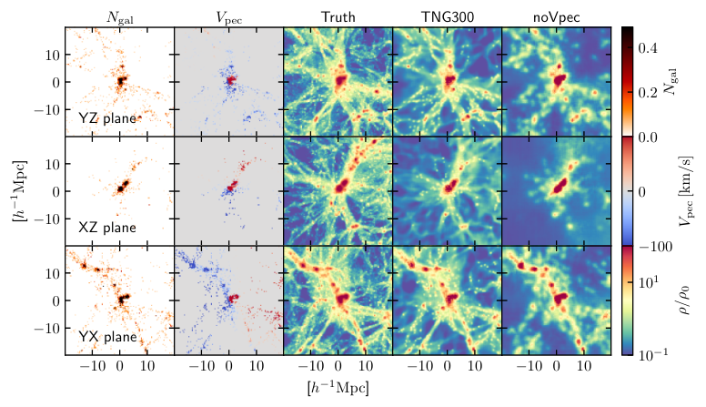
To test the model parameters tuned with TNG100 and TNG300 training sets, we apply the model to the validation samples to compare the resulting dark-matter density cube with the ground truth. Specifically, we use the following four methods for the performance test—visual comparison, joint probability distribution, histogram, and two-point correlation function (2pCF) $\xi(r)=\langle\delta(\mathbf{x})\delta(\mathbf{x}+\mathbf{r})\rangle_{\mathbf{x}}$ . To examine the performance of the each model, we use the Kolmogorov-Smirnov statistics of the 2pCFs between truth and prediction at a given scale,

Here, $\tilde{P}(\xi^{\prime})=N(\xi<\xi^{\prime})/N_{\rm sample}$ is the empirical distribution function, where $N_{\rm sample}$ and $N(\xi<\xi^{\prime})$ are, respectively, the number of whole samples and the number of those satisfying $\xi<\xi^{\prime}$. The smaller ${\rm KS}(\xi_{\rm pred},\xi_{\rm truth})$ indicates that the predicted probability distribution of the 2pCF is closer to the true distribution, so we use that as a metric to compare the performance of models. For both TNG100 and TNG300, the models at the minimum training loss provide the closest distribution of the 2pCF predictions to their truth, and we adopt them as our optimal models.

Table 2, Figures 4 and 5 show a visual inspection and the statistics of the TNG300 validation samples, which show a good agreement with their true values. Interestingly, the predicted dark matter distribution shows small-scale filamentary structures, which are not apparently shown in $N_{\rm gal}$ alone. This is the first indication of the importance of the (radial) peculiar velocity field for reconstructing the small-scale filamentary structures; that is, the recovered dark-matter map shows much more detailed structure than simply connecting the galaxy positions, since the peculiar velocity could provide information about the underlying gravitational potential. Simply put, we use the galaxies as test particles for recovering the local gravitational field. Note that, however, there is a slight difference in the detailed distribution of filamentary structures between truth and prediction. Also, note that there exists a sharp lower cut in the predicted density $\min\rho_{\rm pred}\sim 10^{-2}\rho_{0}$. The above two issues could be overcome by using higher-resolution hydrodynamic simulations and observational data with more low-brightness galaxies. Also, fine-tuned choices of loss function might help manage an issue about a slight difference of filamentary structures.

After choosing the optimal models, we perform the convergence test between models with different simulation resolutions and setups. First, we compare the local dark-matter density field predictions from TNG100 and TNG300 within the radius $r=10\mathinner{{\rm Mpc}/h}$. We find that they show similar distribution up to $r\sim 4\mathinner{{\rm Mpc}/h}$, while the dark-matter map from TNG100 shows finer small-scale structures than TNG300 (see Section IV.3). Also, we apply the CNN model from TNG100 to the test sample of EAGLE (EAGLE-TNG100 in Table 2).

Note that we do not apply the CNN model from TNG300 to EAGLE because the volume of EAGLE is not sufficiently larger than the volume of TNG300 sub-cubes. We find that its performance test result is similar to the TNG100 validation sample, except that EAGLE-TNG100 tends to slightly overestimate the dark-matter density (see Figure 5 and Table 2).

We also test the performance of various comparison models of TNG300 (see Table 1 for definitions). Most comparison models show similar overall performance to TNG300, while those from the dark-matter-only simulation (DMhalo) has slightly more offset in the distribution of 2pCFs. Those without using the radial peculiar velocity as inputs (noVpec), however, do not reproduce any small-scale filamentary structure shown in the true dark matter distribution (see the right panel of Figure 4). From its visual inspection, one could interpret the output of noVpec as a smoothing of the galaxy number distribution—the only available input of the given DL model— with a few Mpc-scale. As a result, the 2pCFs of noVpec show a significant deviation from their truth in small scales with $r\lesssim 3\mathinner{{\rm Mpc}/h}$ (see Table 2). From the comparison to TNG300 and its other comparison models, it is apparent that the (radial) peculiar velocity plays a significant role in reconstructing the small-scale filamentary structure.

Figure 6 shows a sliced view of the reconstructed Cosmic Web integrated over $4\mathinner{{\rm Mpc}/h}$ thickness. Each panel shows the Cosmic Web on the plane of the Supergalactic Cartesian coordinates (SGX, SGY, and SGZ), extended to the full cube with the side length of $40\mathinner{{\rm Mpc}/h}$. Figure 6 clearly shows known local objects that we designated by their common name. The figure also recovers known local large-scale structures. For example, we find a $10\mathinner{{\rm Mpc}/h}$-spread along $+{\rm SGY}$-direction in the SGZ-SGY (upper left panel) and SGY-SGX (lower-right panel) planes. This structure is known as Local Sheet, which connects the Local Group and Virgo cluster and contains M81, NGC5194, Canes II, and Coma I groups (Tully et al. 2008; Courtois et al. 2013). We also find that, around the Local Group, the Local Sheet is connected to the Fornax Wall (Fairall et al. 1994), which is a $20\mathinner{{\rm Mpc}/h}$-sized spread along ($-$SGY,$-$SGZ)-direction, containing Fornax cluster, Eridanus cluster, and Dorado group as members (upper-left panel). At the opposite direction to the Fornax Wall on the SGZ-SGY plane, the Local Void (Tully & Fisher 1987) is also apparent (also shown on the SGZ-SGX plane), which might extend beyond the boundary of our local universe sample. In Figure 6, we also present the velocity flow lines derived from the reconstructed gravitational potential gradient with arrows and black lines. The velocity flow shows the motion of material from the Local Void to nearby filamentary structures and clusters such as the Local Sheet, Fornax Wall, and Virgo cluster. Note that we cannot reproduce the velocity flow from the Virgo cluster to the Great Attractor ($+{\rm SGX}$-direction), because of the limited extension of the volume that we analyze here. However, we would like to emphasize that the recovered dark-matter map provides us detailed density and velocity fields around these known local large-scale structures.

The recovered Cosmic Web also shows a hint of new structures that require further investigation. For example, the direction of the Local Sheet is similar to the direction of the so-called vast polar structure (VPOS), which consists of satellite galaxies, globular clusters and stellar streams around the Milky-way galaxy (Pawlowski et al. 2012). As shown in Figure 6, the Local Sheet, being the strongest filamentary structure around the Local Group, is a source of velocity flow; that might cause a connection between the two. Also, a couple of small filaments are visible in our maps, which could be good targets for systematic examination with deep imaging surveys.

Furthermore, to estimate the uncertainties of the dark-matter map, we perform a stress test on our CNN models by incorporating distance measurement uncertainties in the CF3. We use the one standard deviation uncertainty in distance modulus ($\epsilon_{\mu}$) in the CF3,

Here $\epsilon_{i}$ includes the one standard deviation uncertainty determined from a recalibration of galaxy magnitude with H I linewidth (Tully & Courtois 2012), distance measurement of the Tip of the Red Giant Branch from the Hubble Space Telescope, Type Ia supernovae from various samples (Tully et al. 2013), Tully-Fisher relation using Spitzer $[3.6]$ photometry, and the Fundamental Plane relation from the Six Degree Field Galaxy Survey (6dFGS) (Tully et al. 2016). We then generate 1,000 sets of random distance moduli that follow the normal distribution,

Then, we re-calculate the radial peculiar velocity by subtracting the Hubble flow corresponding to the random distances from the $V_{\rm GSR}$. Since the distance measurement error exists only along the radial direction, we have generated the two-dimensional column density map of the dark matter that is less affected by the error than the three-dimensional dark-matter density field (see Figure 9). Also, we find that the dark-matter column density map driven from TNG300 shows significantly less deviation than that of TNG100, which suffers from some spurious structure consistently appearing near the Galactic plane.

The left panels of Figure 7 (labeled as TNG300) show the recovered local dark-matter map on the sky (gray map),

where ${\mathinner{\boldsymbol{\theta}}}$, $r$, $\rho({\mathinner{\boldsymbol{\theta}}},r)$ are the two-dimensional sky coordinates, distance from the observer, and the dark-matter density at the given $({\mathinner{\boldsymbol{\theta}}},r)$, respectively. We use the Healpix (Zonca et al. 2019; Górski et al. 2005) package to reconstruct the two-dimensional sky map from the three-dimensional data cube. We set the resolution parameter ${\rm Nside}=128$, which roughly corresponds to the angular resolution of $27^{\prime}$. This figure also shows the locations and radial peculiar velocities of galaxies that we use for the reconstruction (color-coded dots), as well as the locations of some well-known galaxy groups and clusters (large dots).

The map in Figure 7 uses the radial distance and radial peculiar velocities reported in the Cosmicflows-3 catalog (Tully et al. 2016). We have mitigated the $10-30\%$ uncertainties of distance measurement in the catalog by adopting the radial binning of $\Delta r=4\mathinner{{\rm Mpc}/h}$. We further analyze the statistical uncertainties of the recovered dark-matter map by generating 1,000 realizations incorporating the uncertainties of the distance measurement (see Section IV.2). From the high angular resolution map (${\rm Nside}=128$), we define the angular covariance function,

where $\Sigma_{0}=\rho_{0}\Delta r$ is the mean dark-matter column density, $\langle\ldots\rangle_{N,{\mathinner{\boldsymbol{\theta}}},{\mathinner{\boldsymbol{\theta}}}^{\prime}}$ is the average over $N=$1,000 realizations and sky coordinates ${\mathinner{\boldsymbol{\theta}}}$ and ${\mathinner{\boldsymbol{\theta}}}^{\prime}$ that satisfy $|{\mathinner{\boldsymbol{\theta}}}-{\mathinner{\boldsymbol{\theta}}}^{\prime}|=\delta\theta$, and $\delta\Sigma({\mathinner{\boldsymbol{\theta}}})\equiv\Sigma({\mathinner{\boldsymbol{\theta}}})-\langle\Sigma({\mathinner{\boldsymbol{\theta}}}\rangle_{N}$. We found that the angular covariance function follows an exponential decay over $\delta\theta$,

and the values of the angular scale that shows a strong pixel-to-pixel correlation are $\mathbf{\delta}\theta_{0}=20.7^{\circ}$, $9.71^{\circ}$, $6.53^{\circ}$, $5.04^{\circ}$, and $4.24^{\circ}$, respectively, from the nearest ($r<4\mathinner{{\rm Mpc}/h}$) to the farthest ($16\mathinner{{\rm Mpc}/h}<r<20\mathinner{{\rm Mpc}/h}$) radial bins (see Figure 8). $\delta\theta_{0}$ at different radial bins correspond to the linear scales $\delta\ell=0.26$, $0.68$, $0.92$, $1.06$, and $1.18\mathinner{{\rm Mpc}/h}$, respectively. $\delta\ell$ at the nearest radial bin well represent the spatial resolution of the three-dimensional grid ($0.3215\mathinner{{\rm Mpc}/h}$). On the other hand, $\delta\ell$ at the farthest radial bin may mean a typical scale of the filamentary structure at given radial bin width and galaxy number density. For the statistical analysis, we degrade the angular resolution of each map to $\mathbf{\delta}\theta_{0}$—${\rm Nside}=4$, $8$, $8$, $16$, and $16$ from the nearest to the farthest radial bins— and assume that each pixel in the degraded map is statistically independent.

Figure 9 shows the mean ($\langle\log_{10}\Sigma\rangle$; left panel) and the standard deviation ($\Delta\log_{10}\Sigma$; middle panel) of the logarithm of the local dark-matter column density over 1,000 realizations incorporating the uncertainties of the distance measurement. We find that the standard deviation per pixel stays in the range of $\Delta\log_{10}\Sigma/\Sigma_{0}\simeq 0.1-0.4$, with only a mild dependence to the density contrast. As a result, the signal-to-noise ratio ${\rm SNR}\equiv|\langle\log_{10}\Sigma\rangle|/\Delta\log_{10}\Sigma$ scales almost linearly as the density contrast, reaching up to $\mathbf{{\rm SNR}\simeq}10$ for the density peaks. On average, the signal-to-noise ratios for dark-matter distribution per pixel at higher Galactic latitudes ($|b|>10^{\circ}$) are 4.25, 3.76, 3.94, 4.19, and 4.52, respectively, from the nearest to the farthest radial bin.

Note that, in addition to the distance measurement uncertainty, there are systematic uncertainties in DL mapping itself into the error budget. For example, the galaxy simulations with different resolutions or different sub-grid prescriptions can lead to different DL mapping. We check such systematic effect by comparing TNG300 with various comparison models, including those already introduced in Table 1. To do this, we calculate the on-sky average of the systematics

where $\Sigma$ and $\Sigma_{\mathsf{TNG300}}$ are the local dark-matter column densities from a given comparison model and TNG300, both by adopting the reported values of galaxy locations and peculiar velocities. First, we check the systematic effect of the resolution by comparing the local dark-matter map estimated from TNG100 and TNG300. The top-right panel of Figure 7 shows the $r<4\mathinner{{\rm Mpc}/h}$ bin dark-matter map driven from the high-resolution result (TNG100). TNG100 systematically underestimate the density contrast by $\Delta_{\rm sys}=2.3$ on average (see Table 3).

Secondly, to estimate the systematic effect from different sub-grid prescriptions, we have repeated the deep-learning procedure by using the dark-matter halo samples from the dark-matter-only simulation TNG300-1-Dark by matching the galaxy/halo number density (DMhalo). The right panels of Figure 9 show the difference between the two dark-matter maps in units of standard deviation at each pixel. Even with this extreme comparison between full hydrodynamic simulation and pure $N$-body simulation , we find that systematic effects lead to $\Delta_{\rm sys}=1.7$, $1.4$, $1.2$, $1.1$, and $1.0$ on average from the top (nearest) to the bottom (furthest) maps.

We further test the systematic effect due to different Hubble parameters ($H_{0}=75\,{\rm km/s/Mpc}$; diffH0) and find only $\Delta_{\rm sys}\simeq 0.15$. Different $B$-band magnitude cuts ($M_{B}<-16$ and $-17$; 16mag and 17mag, respectively) and using total stellar mass instead of galaxy number (stellarMass) lead to $\Delta_{\rm sys}\simeq 1$. Most importantly, none of the systematic maps shows a significant correlation with the derived cosmic web structure, ensuring the robustness of the derived dark-matter distribution, or the Cosmic Web (see the right panel of Figure 9).

The most striking feature that we have recovered in this study is the filamentary Cosmic Web that is apparent in Figures 7 and 9. First of all, we find that the radial peculiar velocity information is vital to reconstructing the cosmic web, without which the same DL algorithm can not reproduce the Cosmic Web structure at all. For example, the right panels in Figure 7, indicated by noVpec, show the deep-learning result only using galaxy distributions. Note the absence of the filamentary structure in those maps. We note that the noVpec maps resemble the smoothed version of the galaxy distribution. The deep-learning algorithm with stellar-mass weighted galaxy distribution, without peculiar velocity information, leads to the similarly poor quality map.

Another interesting feature in the map is the dark-matter distribution at lower Galactic latitudes ($|b|<10^{\circ}$) where we do not have any input galaxy data. To our surprise, we find that the averaged signal-to-noise ratios per pixel for this region are $4.18$, $4.73$, $5.31$, $5.80$, and $6.21$, respectively, from the nearest to the farthest radial bin. We, however, anticipate that the theoretical uncertainties for the DL mapping would be most substantial for this region. For example, from the aforementioned studies on systematic uncertainties, we find that, on average, lower Galactic latitudes ($|b|<10^{\circ}$) map suffers about $\delta\Delta_{\rm sys}\simeq 0.5$ more systematical shifts than higher Galactic latitudes ($|b|>10^{\circ}$) map. This is indicated in the top two panels of Figure 7 and the systematic shifts shown in the right panels of Figure 9.

References

- Aaronson (1983) Aaronson, M. 1983, The Astrophysical Journal Letter, 266, L11, doi: 10.1086/183969
- Aartsen et al. (2018) Aartsen, M. G., Ackermann, M., Adams, J., et al. 2018, Eur. Phys. J. C, 78, 831, doi: 10.1140/epjc/s10052-018-6273-3
- Abadi et al. (2015) Abadi, M., Agarwal, A., Barham, P., et al. 2015, TensorFlow: Large-Scale Machine Learning on Heterogeneous Systems. https://www.tensorflow.org/
- Abbott et al. (2018) Abbott, T. M. C., Abdalla, F. B., Alarcon, A., et al. 2018, Physical Review D, 98, 043526, doi: 10.1103/PhysRevD.98.043526
- Ackermann et al. (2015) Ackermann, M., Albert, A., Anderson, B., et al. 2015, Physical Review Letter, 115, 231301, doi: 10.1103/PhysRevLett.115.231301
- Akerib et al. (2017) Akerib, D. S., Alsum, S., Araújo, H. M., et al. 2017, Physical Review Letter, 118, 021303, doi: 10.1103/PhysRevLett.118.021303
- Ammazzalorso et al. (2020) Ammazzalorso, S., Gruen, D., Regis, M., et al. 2020, Physical Review Letter, 124, 101102, doi: 10.1103/PhysRevLett.124.101102
- Anderson et al. (2014) Anderson, L., Aubourg, É., Bailey, S., et al. 2014, Monthly Notices of the Royal Astronomical Society, 441, 24, doi: 10.1093/mnras/stu523
- Arcadi et al. (2018) Arcadi, G., Dutra, M., Ghosh, P., et al. 2018, Eur. Phys. J. C, 78, 203, doi: 10.1140/epjc/s10052-018-5662-y
- Astropy Collaboration et al. (2013) Astropy Collaboration, Robitaille, T. P., Tollerud, E. J., et al. 2013, Astronomy & Astrophysics, 558, A33, doi: 10.1051/0004-6361/201322068
- Astropy Collaboration et al. (2018) Astropy Collaboration, Price-Whelan, A. M., SipHocz, B. M., et al. 2018, aj, 156, 123, doi: 10.3847/1538-3881/aabc4f
- Atlas Collaboration (2019) Atlas Collaboration. 2019, Journal of High Energy Physics, 2019, 142, doi: 10.1007/JHEP05(2019)142
- Bell et al. (2003) Bell, E. F., McIntosh, D. H., Katz, N., & Weinberg, M. D. 2003, The Astrophysical Journal Supplement Series, 149, 289, doi: 10.1086/378847
- Camps et al. (2018) Camps, P., Trčka, A., Trayford, J., et al. 2018, The Astrophysical Journal Supplement Series, 234, 20, doi: 10.3847/1538-4365/aaa24c
- Carlesi et al. (2016) Carlesi, E., Sorce, J. G., Hoffman, Y., et al. 2016, Monthly Notices of the Royal Astronomical Society, 458, 900, doi: 10.1093/mnras/stw357
- Carrick et al. (2015) Carrick, J., Turnbull, S. J., Lavaux, G., & Hudson, M. J. 2015, Monthly Notices of the Royal Astronomical Society, 450, 317, doi: 10.1093/mnras/stv547
- Chollet et al. (2015) Chollet, F., et al. 2015, Keras, https://keras.io
- Clowe et al. (2006) Clowe, D., Bradač, M., Gonzalez, A. H., et al. 2006, The Astrophysical Journal Letter, 648, L109, doi: 10.1086/508162
- Cooke et al. (2014) Cooke, R. J., Pettini, M., Jorgenson, R. A., Murphy, M. T., & Steidel, C. C. 2014, The Astrophysical Journal, 781, 31, doi: 10.1088/0004-637x/781/1/31
- Courtois et al. (2013) Courtois, H. M., Pomarède, D., Tully, R. B., Hoffman, Y., & Courtois, D. 2013, The Astronomical Journal, 146, 69, doi: 10.1088/0004-6256/146/3/69
- Crain et al. (2015) Crain, R. A., Schaye, J., Bower, R. G., et al. 2015, Monthly Notices of the Royal Astronomical Society, 450, 1937, doi: 10.1093/mnras/stv725
- Davis et al. (1985) Davis, M., Efstathiou, G., Frenk, C. S., & White, S. D. M. 1985, The Astrophysical Journal, 292, 371, doi: 10.1086/163168
- Desjacques et al. (2018) Desjacques, V., Jeong, D., & Schmidt, F. 2018, Physics Reports, 733, 1, doi: 10.1016/j.physrep.2017.12.002
- Fairall et al. (1994) Fairall, A. P., Paverd, W. R., & Ashley, R. P. 1994, in Astronomical Society of the Pacific Conference Series, Vol. 67, Unveiling Large-Scale Structures Behind the Milky Way, ed. C. Balkowski & R. C. Kraan-Korteweg, 21
- Fang et al. (2020) Fang, K., Banerjee, A., Charles, E., & Omori, Y. 2020, arXiv e-prints, arXiv:2002.06234. https://arxiv.org/abs/2002.06234
- Fornasa et al. (2016) Fornasa, M., Cuoco, A., Zavala, J., et al. 2016, Physical Review D, 94, 123005, doi: 10.1103/PhysRevD.94.123005
- Gardner et al. (2006) Gardner, J. P., Mather, J. C., Clampin, M., et al. 2006, Space Science Reviews, 123, 485, doi: 10.1007/s11214-006-8315-7
- Giesen et al. (2015) Giesen, G., Boudaud, M., Génolini, Y., et al. 2015, Journal of Cosmology and Astroparticle Physics, 2015, 023, doi: 10.1088/1475-7516/2015/09/023
- Glorot et al. (2011) Glorot, X., Bordes, A., & Bengio, Y. 2011, in Proceedings of the fourteenth international conference on artificial intelligence and statistics, 315–323
- Górski et al. (2005) Górski, K. M., Hivon, E., Banday, A. J., et al. 2005, The Astrophysical Journal, 622, 759, doi: 10.1086/427976
- Gottloeber et al. (2010) Gottloeber, S., Hoffman, Y., & Yepes, G. 2010, arXiv e-prints, arXiv:1005.2687. https://arxiv.org/abs/1005.2687
- Hahnloser et al. (2000) Hahnloser, R. H. R., Sarpeshkar, R., Mahowald, M. A., Douglas, R. J., & Seung, H. S. 2000, Nature, 405, 947, doi: 10.1038/35016072
- Harris et al. (2020) Harris, C. R., Millman, K. J., van der Walt, S. J., et al. 2020, Nature, 585, 357, doi: 10.1038/s41586-020-2649-2
- Huchra et al. (2012) Huchra, J. P., Macri, L. M., Masters, K. L., et al. 2012, The Astrophysical Journal Supplement Series, 199, 26, doi: 10.1088/0067-0049/199/2/26
- Hunter (2007) Hunter, J. D. 2007, Computing in Science Engineering, 9, 90, doi: 10.1109/MCSE.2007.55
- Ioffe & Szegedy (2015) Ioffe, S., & Szegedy, C. 2015, arXiv e-prints, arXiv:1502.03167. https://arxiv.org/abs/1502.03167
- Jasche et al. (2015) Jasche, J., Leclercq, F., & Wandelt, B. D. 2015, Journal of Cosmology and Astroparticle Physics, 2015, 036, doi: 10.1088/1475-7516/2015/01/036
- Jasche & Wandelt (2013) Jasche, J., & Wandelt, B. D. 2013, Monthly Notices of the Royal Astronomical Society, 432, 894, doi: 10.1093/mnras/stt449
- Jeffrey et al. (2020) Jeffrey, N., Lanusse, F., Lahav, O., & Starck, J.-L. 2020, Monthly Notices of the Royal Astronomical Society, 492, 5023, doi: 10.1093/mnras/staa127
- Jones et al. (2001) Jones, E., Oliphant, T., Peterson, P., et al. 2001
- Kingma & Ba (2014) Kingma, D. P., & Ba, J. 2014, arXiv e-prints, arXiv:1412.6980. https://arxiv.org/abs/1412.6980
- Kourkchi et al. (2020) Kourkchi, E., Courtois, H. M., Graziani, R., et al. 2020, The Astronomical Journal, 159, 67, doi: 10.3847/1538-3881/ab620e
- Larson et al. (2011) Larson, D., Dunkley, J., Hinshaw, G., et al. 2011, The Astrophysical Journal Supplement Series, 192, 16, doi: 10.1088/0067-0049/192/2/16
- Lavaux & Hudson (2011) Lavaux, G., & Hudson, M. J. 2011, Monthly Notices of the Royal Astronomical Society, 416, 2840, doi: 10.1111/j.1365-2966.2011.19233.x
- Lavaux & Jasche (2016) Lavaux, G., & Jasche, J. 2016, Monthly Notices of the Royal Astronomical Society, 455, 3169, doi: 10.1093/mnras/stv2499
- Libeskind et al. (2010) Libeskind, N. I., Yepes, G., Knebe, A., et al. 2010, Monthly Notices of the Royal Astronomical Society, 401, 1889, doi: 10.1111/j.1365-2966.2009.15766.x
- Licquia & Newman (2015) Licquia, T. C., & Newman, J. A. 2015, The Astrophysical Journal, 806, 96, doi: 10.1088/0004-637X/806/1/96
- Marinacci et al. (2018) Marinacci, F., Vogelsberger, M., Pakmor, R., et al. 2018, Monthly Notices of the Royal Astronomical Society, 480, 5113, doi: 10.1093/mnras/sty2206
- Milletari et al. (2016) Milletari, F., Navab, N., & Ahmadi, S.-A. 2016, arXiv e-prints, arXiv:1606.04797. https://arxiv.org/abs/1606.04797
- Modi et al. (2018) Modi, C., Feng, Y., & Seljak, U. 2018, Journal of Cosmology and Astroparticle Physics, 2018, 028, doi: 10.1088/1475-7516/2018/10/028
- Naiman et al. (2018) Naiman, J. P., Pillepich, A., Springel, V., et al. 2018, Monthly Notices of the Royal Astronomical Society, 477, 1206, doi: 10.1093/mnras/sty618
- Nelson et al. (2018) Nelson, D., Pillepich, A., Springel, V., et al. 2018, Monthly Notices of the Royal Astronomical Society, 475, 624, doi: 10.1093/mnras/stx3040
- Nelson et al. (2019) Nelson, D., Springel, V., Pillepich, A., et al. 2019, Computational Astrophysics and Cosmology, 6, 2, doi: 10.1186/s40668-019-0028-x
- Paturel et al. (2003) Paturel, G., Petit, C., Prugniel, P., et al. 2003, Astronomy & Astrophysics, 412, 45, doi: 10.1051/0004-6361:20031411
- Pawlowski et al. (2012) Pawlowski, M. S., Pflamm-Altenburg, J., & Kroupa, P. 2012, Monthly Notices of the Royal Astronomical Society, 423, 1109, doi: 10.1111/j.1365-2966.2012.20937.x
- Pillepich et al. (2018) Pillepich, A., Nelson, D., Hernquist, L., et al. 2018, Monthly Notices of the Royal Astronomical Society, 475, 648, doi: 10.1093/mnras/stx3112
- Planck Collaboration et al. (2018) Planck Collaboration, Aghanim, N., Akrami, Y., et al. 2018, arXiv e-prints, arXiv:1807.06209. https://arxiv.org/abs/1807.06209
- Ronneberger et al. (2015) Ronneberger, O., Fischer, P., & Brox, T. 2015, arXiv e-prints, arXiv:1505.04597. https://arxiv.org/abs/1505.04597
- Rubin & Ford (1970) Rubin, V. C., & Ford, W. Kent, J. 1970, The Astrophysical Journal, 159, 379, doi: 10.1086/150317
- Schaye et al. (2015) Schaye, J., Crain, R. A., Bower, R. G., et al. 2015, Monthly Notices of the Royal Astronomical Society, 446, 521, doi: 10.1093/mnras/stu2058
- Shandera et al. (2018) Shandera, S., Jeong, D., & Grasshorn Gebhardt, H. S. 2018, Physical Review Letter, 120, 241102, doi: 10.1103/PhysRevLett.120.241102
- Shirasaki et al. (2019) Shirasaki, M., Yoshida, N., & Ikeda, S. 2019, Physical Review D, 100, 043527, doi: 10.1103/PhysRevD.100.043527
- Smith (2015) Smith, L. N. 2015, arXiv e-prints, arXiv:1506.01186. https://arxiv.org/abs/1506.01186
- Springel et al. (2018) Springel, V., Pakmor, R., Pillepich, A., et al. 2018, Monthly Notices of the Royal Astronomical Society, 475, 676, doi: 10.1093/mnras/stx3304
- Springob et al. (2014) Springob, C. M., Magoulas, C., Colless, M., et al. 2014, Monthly Notices of the Royal Astronomical Society, 445, 2677, doi: 10.1093/mnras/stu1743
- Tröster et al. (2017) Tröster, T., Camera, S., Fornasa, M., et al. 2017, Monthly Notices of the Royal Astronomical Society, 467, 2706, doi: 10.1093/mnras/stx365
- Tully & Courtois (2012) Tully, R. B., & Courtois, H. M. 2012, The Astrophysical Journal, 749, 78, doi: 10.1088/0004-637X/749/1/78
- Tully et al. (2016) Tully, R. B., Courtois, H. M., & Sorce, J. G. 2016, The Astronomical Journal, 152, 50, doi: 10.3847/0004-6256/152/2/50
- Tully & Fisher (1987) Tully, R. B., & Fisher, J. R. 1987, Atlas of Nearby Galaxies (Cambridge University Press)
- Tully et al. (2008) Tully, R. B., Shaya, E. J., Karachentsev, I. D., et al. 2008, The Astrophysical Journal, 676, 184, doi: 10.1086/527428
- Tully et al. (2013) Tully, R. B., Courtois, H. M., Dolphin, A. E., et al. 2013, The Astronomical Journal, 146, 86, doi: 10.1088/0004-6256/146/4/86
- Van Der Walt et al. (2011) Van Der Walt, S., Colbert, S. C., & Varoquaux, G. 2011, Computing in science & engineering, 13, 22
- Vannerom (2019) Vannerom, D. 2019, Proc. Sci., DIS2019, 111, doi: 10.22323/1.352.0111
- Virtanen et al. (2020) Virtanen, P., Gommers, R., Oliphant, T. E., et al. 2020, Nature Methods, 17, 261, doi: 10.1038/s41592-019-0686-2
- Wes McKinney (2010) Wes McKinney. 2010, in Proceedings of the 9th Python in Science Conference, ed. Stéfan van der Walt & Jarrod Millman, 56 – 61, doi: 10.25080/Majora-92bf1922-00a
- Wilman & Erwin (2012) Wilman, D. J., & Erwin, P. 2012, The Astrophysical Journal, 746, 160, doi: 10.1088/0004-637X/746/2/160
- Zonca et al. (2019) Zonca, A., Singer, L., Lenz, D., et al. 2019, J. Open Sour. Soft., 4, 1298, doi: 10.21105/joss.01298
- Zwicky (1933) Zwicky, F. 1933, Helv. Phys. Acta, 6, 110