Multiple Code Hashing for Efficient Image Retrieval
Abstract
Due to its low storage cost and fast query speed, hashing has been widely used in large-scale image retrieval tasks. Hash bucket search returns data points within a given Hamming radius to each query, which can enable search at a constant or sub-linear time cost. However, existing hashing methods cannot achieve satisfactory retrieval performance for hash bucket search in complex scenarios, since they learn only one hash code for each image. More specifically, by using one hash code to represent one image, existing methods might fail to put similar image pairs to the buckets with a small Hamming distance to the query when the semantic information of images is complex. As a result, a large number of hash buckets need to be visited for retrieving similar images, based on the learned codes. This will deteriorate the efficiency of hash bucket search. In this paper, we propose a novel hashing framework, called multiple code hashing (MCH), to improve the performance of hash bucket search. The main idea of MCH is to learn multiple hash codes for each image, with each code representing a different region of the image. Furthermore, we propose a deep reinforcement learning algorithm to learn the parameters in MCH. To the best of our knowledge, this is the first work that proposes to learn multiple hash codes for each image in image retrieval. Experiments demonstrate that MCH can achieve a significant improvement in hash bucket search, compared with existing methods that learn only one hash code for each image.
1 Introduction
With the rapid growth of multimedia applications [50, 11, 51, 43, 44, 57, 70, 45, 60, 66, 69, 74, 64, 63, 65, 62, 59, 65, 59, 39, 67, 29], large-scale and high-dimensional image data has brought much burden to the search engines. To ensure search efficiency, approximate nearest neighbor (ANN) [12, 8, 1, 68, 61, 52] search plays a fundamental role. As a popular solution of ANN search, hashing [12, 23, 13, 56, 46, 22, 26, 49, 53, 71, 31, 35, 38, 15, 58, 36, 16, 37] has attracted much attention in recent years.
The goal of hashing is to represent the data points as compact similarity-preserving binary hash codes in Hamming space [41, 47, 5]. Based on hash code representations, the storage cost can be dramatically reduced. Furthermore, we can adopt two procedures, i.e., Hamming ranking and hash bucket search [34, 32, 7], to accelerate search speed. The Hamming ranking procedure obtains a ranking list according to the Hamming distance between query and database points. The computational complexity of this procedure is [2], where is the number of database points. The hash bucket search procedure reorganizes the learned hash codes as a hash table (index). Based on the hash index, hash bucket search can enable a sub-linear or even constant search by returning data points in those hash buckets whose Hamming distance to the query is smaller or equal to a given Hamming radius. In real applications, hash bucket search is typically more practical than Hamming ranking for fast search, especially for cases with a large-scale database.

Over the past decades, many hashing methods [13, 46, 3] have been proposed for image retrieval. However, all existing methods learn only one hash code for each image. When the semantic information of the images is complex, these methods may fail to put similar image pairs into the same hash bucket. An example for illustrating the shortcoming of existing hashing methods is shown in Figure 1. Suppose that there exists an image that contains both a dog and a cat in the database, i.e., image (c) in Figure 1. There are also two image queries that contain a dog and a cat separately, i.e., image (a) and image (b) in Figure 1. Suppose that we use -bit binary hash codes to represent images. The category “dog” and category “cat” are represented by “010” and “101”, respectively. For image (c), we can find that no matter which hash bucket it is mapped to, it cannot be directly retrieved (without bit flipping) by these two queries at the same time. To get image (c) as a search result for these two queries, we have to enlarge the search Hamming radius. For hash bucket search, the search cost will increase exponentially if we enlarge the search Hamming radius. In other words, the search efficiency will be significantly deteriorated.
In this paper, we propose a novel hashing framework, called multiple code hashing (MCH), for image retrieval. The main contributions of this paper are summarized as follows:
- •
MCH learns multiple hash codes for each image, with each code representing a different region of the image. To the best of our knowledge, MCH is the first hashing method that can learn multiple hash codes for each image. By representing each image with multiple hash codes, MCH can keep the Hamming distance of similar image pairs small enough and enable efficient hash bucket search.
- •
A novel deep reinforcement learning algorithm is proposed to learn the parameters in MCH. In particular, an agent is trained in MCH to explore different regions of the image that can better preserve the pairwise similarity than the whole image.
- •
MCH is a flexible framework that decomposes the multiple hash codes learning procedure into two steps: base hashing model learning step and agent learning step. This decomposition simplifies the learning procedure and enables the easy integration of different kinds of base hashing models.
- •
Extensive experiments demonstrate that our MCH can achieve a significant improvement in hash bucket search, compared with existing hashing methods that learn only one hash code for each image.
2 Related Work
In this section, we briefly review the related work, including hash bucket search and deep reinforcement learning.
2.1 Hash Bucket Search
Hash bucket search is an efficient method to locate the nearest codes in Hamming space. Given a hash code, it costs time to locate its corresponding hash bucket. Ideally, if the data points in this bucket can satisfy the requirement of the search, the time cost of the hash bucket search is . If there are not enough data points in this bucket, we need to expand the Hamming radius by flipping bits to visit more hash buckets. In the worst case, all buckets are visited and the search cost will be , where denotes the hash code length. A general procedure of hash bucket search [2] is summarized in Algorithm 1. We can find that when the Hamming radius increases, the number of hash buckets need to be visited increases exponentially, which will severely deteriorate the retrieval efficiency in online search.
2.2 Deep Reinforcement Learning
Reinforcement learning is a problem concerned with how an agent ought to learn behavior through trial-and-error interactions in a dynamic environment [20]. Due to the recent development of deep learning, deep reinforcement learning has attracted much attention and obtained progressive results [40, 48]. More recently, deep reinforcement learning has been introduced to image hashing applications. Deep reinforcement learning approach for image hashing (DRLIH) [72] was proposed to learn hash functions in a sequential process. In [10], GraphBit was designed to mine the reliability of hash codes. These methods generate only one hash code for the whole image. None of them can generate multiple hash codes for modeling complex semantic information in images. Furthermore, these methods utilize deep reinforcement learning to generate high-quality hash codes, while our MCH utilizes deep reinforcement learning to explore different regions of the image that can better preserve the pairwise similarity than the whole image.
3 Notation and Problem Definition
3.1 Notation
In this paper, we use boldface lowercase letters like to denote vectors and boldface uppercase letters like to denote matrices. denotes the -norm for vector . denotes the element in the -th row and -th column of the matrix . denotes the the cosine distance between vector and vector . is an element-wise sign function which returns if the element is positive and returns otherwise.
3.2 Problem Definition
In this paper, we only focus on the setting with pairwise labels [33, 4, 3, 21]. The technique in this paper can also be adapted to settings with other supervised information that includes pointwise labels [46], triplet labels [25, 73] and ranking labels [54, 14]. This will be pursued in our future work.
Suppose we have training samples which are denoted as . Furthermore, the pairwise labels of the training set are also provided. The pairwise labels are denoted as: , where if and are similar, otherwise if and are dissimilar.
The goal of MCH is to learn a hash function , where denotes the number of hash codes11 1 We represent the hash code as a vector form of for convenience of learning. After learning, we can easily transform the learned hash code to the form of . and each . The hash function encodes each data point into -bit hash codes, which aims to represent the complex semantic information in the images to enable efficient hash bucket search.
4 Multiple Code Hashing
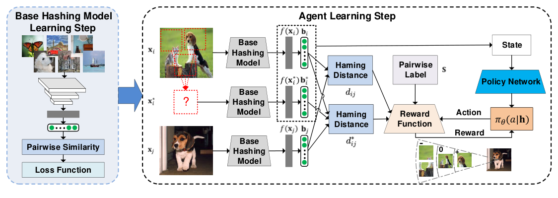
In this section, we present the details about our MCH framework, including base hashing model learning step and agent learning step, which is illustrated in Figure 2.
4.1 Base Hashing Model Learning Step
The base hashing model in MCH is used to learn one hash code for a region of the image or the whole image. Both shallow hashing models and deep hashing models can be used as the base hashing model in MCH. Given an image , a shallow hashing model can first extract its hand-crafted features or utilize a backbone network to extract its features and then learn a linear or non-linear mapping followed by function to get its hash code . A deep hashing model can use raw pixels in image as the input and get its hash code by end-to-end representation learning and hash coding. The Hamming distance between hash codes and can be calculated as follows:
| (1) |
To preserve the similarity between the data points, the Hamming distance between hash codes and should be relatively small if , while relatively large if . In other words, the goal of a hashing model is to solve the following problem:
| (2) |
where is a loss function and denotes the parameters in that need to be learned. Our MCH is flexible enough to integrate different base hashing models with different types of loss functions . We adopt five different kinds of existing hashing methods as the base hashing models in this paper, which are listed in Table 1. Other existing hashing methods can also be adopted as base hashing models in MCH in a similar way as those in Table 1, which will not be further discussed because this is not the focus of this paper.
All the loss functions in Table 1 are defined on the Hamming distance of data pairs. Kernel-based supervised hashing (KSH) [33] uses loss function. Since the discrete optimization problem is hard to solve, KSH replaces with Sigmoid function to get relaxed hash codes. HashNet [4], asymmetric deep supervised hashing (ADSH), deep Cauchy hashing (DCH) [3] and maximum-margin Hamming hashing (MMHH) [21] are recently proposed deep hashing methods. Similar to KSH, HashNet utilizes Tanh function to get relaxed hash codes. ADSH, DCH and MMHH solve the discrete optimization problem by relaxing to a continuous vector with a constraint that . Such relaxation will cause a quantization error and reduce the quality of hash codes. To learn high-quality hash codes, the regularization term should be taken into consideration in the optimization problem. in the loss functions of HashNet, DCH and MMHH is the weight for each training pair. in the loss functions are hyper-parameters set by the corresponding authors.
4.2 Agent Learning Step
The agent learning step is used to learn multiple hash codes for each image with the base hashing model and reinforcement learning.
As shown in Figure 2, a region is randomly cropped from image . Then the features and hash codes for both and are provided through the base hashing model. The goal of agent learning is to determine whether the hash code should be kept as one of the multiple hash codes for image .
State Space: Given an image and a cropped region , the state vector is the concatenation of the feature vectors , , and the hash codes of and region . This process can be formulated as follows:
| (3) |
where denotes the vector concatenation operation on and . More specifically, suppose each image is embedded into a -dimensional feature vector and the length of the hash code is , then the dimension of the state vector is .
Action Space: Given the current state vector , the agent aims to select one action to keep or discard the hash code . The action has the following two possible choices:
| (4) |
Reward Function: Given the sampled action , the reward function can be calculated based on the loss function defined in (2). First, we redefine the asymmetric Hamming distance from to when keeping the hash code as follows:
| (5) |
which is consistent with the procedure of the hash bucket search. We can treat as the query, as a data point in the database and as two hash codes for in Algorithm 1. In other words, is located in two different hash buckets, and the hash bucket with a smaller Hamming distance to will be visited first, which indicates that will be successfully retrieved. We define the following reward function to reflect the influence of the hash code on the similarity preservation of data point .
| (6) |
If the agent discards the hash code (), the reward is which means it does not affect the hash bucket search. When the agent keeps (), the reward will be positive if the newly kept hash code can better represent the semantic information of image and lead to a lower loss for similarity preservation. Otherwise, the reward will be negative to force the agent to discard the meaningless hash code.
Policy Network: We employ a multi-layer perceptron (MLP) with a Softmax layer in the end as our policy network. More specifically, the policy network has five fully-connected layers. We apply ReLU as the activation function. We also perform Batch Normalization [18] to accelerate the training of the policy network. The input of the policy network is the state vector and the output is the predicted distribution of the action , which is denoted as , where is the parameter of the policy network.
The goal of the policy network is to maximize the expected reward for the multiple hash code decision processes. We utilize the REINFORCE algorithm [55] to obtain the gradient of , which is formulated as follows:
| (7) |
In MCH, the parameters need to be learned contain and . We first learn the parameter by training the base hashing model. Then in order to maximize the expected reward in (7), we adopt a back-propagation algorithm to learn the parameter . The overall learning procedure is summarized in Algorithm 2.
4.3 Out-of-Sample Extension
After we have completed the whole learning procedure, we can only get the base hashing model and the agent. We still need to perform out-of-sample extension to predict the multiple hash codes for images unseen in the training set.
For any new image unseen in the training set, in addition to the original image, we crop regions (four corners and one middle) from . The crop ratio is controlled by , which is a hyper-parameter. We use such a cropping strategy just for demonstrating the effectiveness of our MCH in this paper. The cropping strategy can be adjusted according to actual needs. First, we utilize the learned base hashing model to obtain the hash codes of image and all its cropped regions. Then we utilize the policy network to calculate the probability of keeping each hash code. Once the probability is larger than a given threshold of , which is also a hyper-parameter, the corresponding hash code will be kept. Here, the probability of keeping the hash code for the original image is fixed to to ensure that any image has at least one hash code.
5 Experiments
In this section, we conduct extensive evaluations of the proposed method on three widely used benchmark datasets. To prove the effectiveness of MCH, we adopt five different kinds of existing hashing methods as the base hashing models and illustrate the improvements brought by MCH, in terms of both accuracy and efficiency.
5.1 Datasets
We select three widely used benchmark datasets for evaluation. They are NUS-WIDE [6], MS-COCO [30] and MIR FLICKR [17].
NUS-WIDE dataset contains images collected from the web, with each data point annotated with as least one class label from categories. Following [27], we use the subset belonging to the most frequent classes. We randomly select images per class as the query set ( images in total). The remaining images are used as the database set, from which we randomly sample images per class as the training set ( images in total).
MS-COCO contains training images and validation images. Each image is annotated with some of the semantic concepts. Following [3], we randomly select images as the query set. The remaining images are used as database set, and we randomly sample images from the database for training.
MIR FLICKR dataset contains images. Each image is annotated with multiple labels based on unique classes. We randomly select images as the query set. The remaining images are used as the database set, from which we randomly sample images as the training set.
As the data point might belong to multiple categories, following [28, 27, 3], two data points that have at least one common semantic label are considered similar.
5.2 Experimental Setup
5.2.1 Baselines and Evaluation Protocol
Both shallow hashing methods and deep hashing methods are adopted as baselines for comparison. Shallow hashing methods include unsupervised and supervised methods. Unsupervised shallow hashing methods consist of locality-sensitive hashing (LSH) [12] and iterative quantization (ITQ) [13]. Supervised shallow method is kernel-based supervised hashing (KSH) [33]. Deep hashing methods consist of HashNet [4], asymmetric deep supervised hashing (ADSH), deep Cauchy hashing (DCH) [3] and maximum-margin Hamming hashing (MMHH) [21]. To demonstrate that our MCH is an effective and flexible framework, we adopt both shallow hashing methods and deep hashing methods including KSH, HashNet, ADSH, DCH and MMHH as the base hashing model in MCH. The corresponding MCH methods are called “MCH-KSH”, “MCH-HashNet”, “MCH-ADSH”, “MCH-DCH” and “MCH-MMHH”, respectively.
To verify that MCH can enable the similar data points to fall into the Hamming ball within radius , we adopt recall within Hamming radius (R@H) and precision within Hamming radius (P@H) to evaluate MCH and baselines. We also adopt the widely used mean average precision (mAP) to measure the accuracy of our MCH and baselines. To evaluate the efficiency in the hash bucket search, we report F1-bucket curves to compare MCH and baselines. More specifically, we conduct the hash bucket search with different settings of , which is defined in Algorithm 1. Then for each setting of , we draw the F1 score and the number of hash buckets that need to be visited as a point. Finally, we connect these points in an ascending order of to get F1-bucket curves. Moreover, we report the average number of hash codes (ANHC) for MCH which reflects the average number of hash codes that MCH learns for an image. We can calculate the ANHC as follows:
| (8) |
where denotes the probability that the -th region of the -th image will be kept, is the threshold defined in Section 4.3, and is an indicator function. if is true otherwise .
5.2.2 Implementation Details
Our implementation of MCH is based on PyTorch [42]. For shallow hashing methods, we use the -dimensional features extracted by AlexNet [24] pre-trained on ImageNet [9] as image features. For deep hashing methods, we use original images as input and adopt AlexNet as the backbone architecture for a fair comparison. We fine-tune convolutional layers conv1-conv5 and fully-connected layers fc6-fc7 of AlexNet pre-trained on ImageNet and train the last hash layer, all through back-propagation. We use mini-batch stochastic gradient descent (SGD) with momentum for training the policy network and choose the learning rate from . The initial learning rate is set to and the weight decay parameter is set to . The total iteration number is set to . The size of each mini-batch is set to . The hyper-parameters of the base hashing model are set by following the suggestions of the corresponding authors. All the hyper-parameters shared by MCH and its base hashing model are kept the same for a fair comparison. We select the unique hyper-parameters of our MCH based on results of a validation strategy.
All experiments are run on a workstation with Intel(R) Xeon(R) Gold 6240 CPU@GHz of cores, G RAM and GeForce RTX 2080 Ti GPU cards. Furthermore, all experiments are run for five times with different random seeds and the average value is reported.
| Method | NUS-WIDE | MS-COCO | MIR FLICKR | |||||||||
| 16 bits | 32 bits | 48 bits | 64 bits | 16 bits | 32 bits | 48 bits | 64 bits | 16 bits | 32 bits | 48 bits | 64 bits | |
| LSH | 0.3449 | 0.3653 | 0.3815 | 0.3861 | 0.3660 | 0.3763 | 0.3880 | 0.3947 | 0.5710 | 0.5799 | 0.5908 | 0.5931 |
| ITQ | 0.5183 | 0.5140 | 0.5172 | 0.5185 | 0.4589 | 0.4711 | 0.4788 | 0.4826 | 0.6479 | 0.6516 | 0.6536 | 0.6544 |
| KSH | 0.6894 | 0.7003 | 0.7047 | 0.7062 | 0.5614 | 0.5768 | 0.5821 | 0.5866 | 0.7923 | 0.8005 | 0.8024 | 0.8038 |
| MCH-KSH | 0.6955 | 0.7062 | 0.7104 | 0.7128 | 0.5691 | 0.5858 | 0.5915 | 0.5967 | 0.8051 | 0.8110 | 0.8117 | 0.8114 |
| HashNet | 0.7064 | 0.7184 | 0.7211 | 0.7225 | 0.5766 | 0.5859 | 0.5886 | 0.5846 | 0.8454 | 0.8515 | 0.8531 | 0.8540 |
| MCH-HashNet | 0.7098 | 0.7221 | 0.7246 | 0.7266 | 0.5800 | 0.5901 | 0.5929 | 0.5887 | 0.8491 | 0.8553 | 0.8563 | 0.8573 |
| ADSH | 0.7161 | 0.7391 | 0.7444 | 0.7461 | 0.5643 | 0.5934 | 0.6055 | 0.6135 | 0.8352 | 0.8452 | 0.8471 | 0.8470 |
| MCH-ADSH | 0.7179 | 0.7403 | 0.7454 | 0.7471 | 0.5684 | 0.5985 | 0.6098 | 0.6174 | 0.8383 | 0.8475 | 0.8502 | 0.8511 |
| DCH | 0.6804 | 0.6796 | 0.6765 | 0.6761 | 0.5542 | 0.5554 | 0.5550 | 0.5546 | 0.8273 | 0.8267 | 0.8251 | 0.8214 |
| MCH-DCH | 0.6832 | 0.6840 | 0.6819 | 0.6801 | 0.5607 | 0.5665 | 0.5650 | 0.5647 | 0.8359 | 0.8348 | 0.8280 | 0.8230 |
| MMHH | 0.6762 | 0.6762 | 0.6716 | 0.6702 | 0.5499 | 0.5498 | 0.5456 | 0.5442 | 0.8199 | 0.8120 | 0.8119 | 0.8091 |
| MCH-MMHH | 0.6791 | 0.6818 | 0.6795 | 0.6763 | 0.5563 | 0.5597 | 0.5547 | 0.5492 | 0.8276 | 0.8200 | 0.8162 | 0.8138 |
5.3 Accuracy
The recall and precision within Hamming radius reflect the performance for retrieving top-ranking data points by the hash bucket search at time cost. The recall within Hamming radius is shown in Figure 3. We can find that MCH achieves much better results than its base hashing model on all benchmark datasets with regard to different code lengths. This verifies that MCH can make more similar data points fall into the Hamming ball within radius to the query and enable more efficient retrieval of top-ranking data points. Figure 4 shows the precision within Hamming radius . We can find that MCH can also improve the precision within Hamming radius , compared with its base hashing model. This verifies that MCH will not reduce the accuracy of retrieving top-ranking data points.
The mAP results of all methods are listed in Table 2, which show that MCH can achieve better accuracy than its base hashing model. Please note that our MCH is mainly designed to improve the efficiency of hash bucket search. The improvement in mAP is to illustrate that our MCH will not reduce accuracy.
To verify the efficiency of MCH in hash bucket search, F1-bucket curves of all methods with different code lengths are illustrated in Figure 5, Figure 6 and Figure 7, respectively. The results show that MCH can perform much more efficient hash bucket search than the base hashing model. Specifically, compared to KSH, the best shallow hashing method with deep features as input, MCH-KSH can obtain the same F1 score while greatly reducing the number of hash buckets that need to be visited. The F1-bucket curves also show some interesting phenomenons.
(1) Without modeling the pairwise similarity information, unsupervised shallow hashing methods are worse than supervised hashing methods. (2) ADSH treats query points and database points in an asymmetric way. In most situations, ADSH achieves more efficient hash bucket search, compared with symmetric supervised hashing methods. (3) Different symmetric supervised hashing methods have large distinctions in the efficiency of hash bucket search. The reason is that different types of loss functions impose distinct penalties for similar point pairs () [3]. These observations may give some insights about designing new hashing methods for more efficient hash bucket search.5.4 Visualization Study
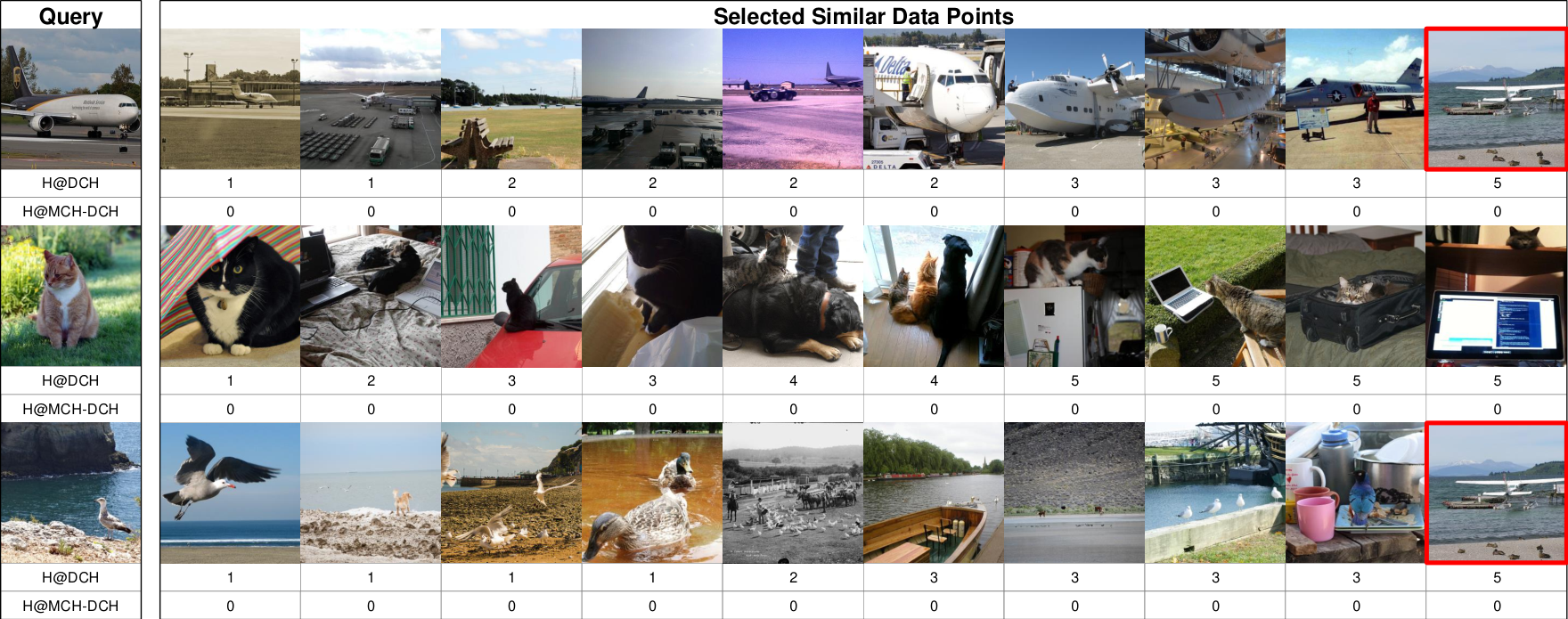
We perform a visualization study on MS-COCO dataset to give an intuition about why MCH can outperform existing methods. We randomly select some query images from the query set and select similar data points for each query from the database set. We choose DCH as the base hashing model of MCH and set the code length to bits. Results are shown in Figure 8, in which the first column denotes the query, and the following columns denote the retrieved data points to the query. The Hamming distance between the query and each retrieved data point is also shown in Figure 8. The results show that our MCH can better represent the data points with complex semantic information and enable more similar data points to fall into the Hamming ball within radius to the query. There also exists an image in the database set describing both the airplane and the bird. Our MCH can enable it to appear in multiple hash buckets simultaneously. Hence, it can be retrieved in time by queries of different categories. This validates that MCH can enable more efficient hash bucket search.
5.5 Sensitivity to Hyper-Parameter
Since the hash bucket search efficiency is the main focus of this paper, we study the sensitivity of the hyper-parameters and on the hash bucket search efficiency. The efficiency (F1-bucket) of MCH-DCH and DCH with code length being bits are shown in Figure 9. From Figure 9 (a), we can see that MCH is not sensitive to in the range . To further analyze the sensitivity to , we select queries that include the “Airplane” category and report the F1-bucket curves in Figure 9 (b) using only these selected queries. We can see that MCH is not sensitive to in the range . We also select queries that include “Bird” category and results are shown in Figure 9 (c). We can find that the hyper-parameter sensitivity results are similar to those using all queries. From Figure 9 (d), we can see that MCH is not sensitive to in the range .
We also report the average number of hash codes of MCH-DCH in Table 3. Please note that when , MCH-DCH will degenerate to its base hashing model DCH. We can find that a more efficient hash bucket search in Figure 9 can be achieved with a larger average number of hash codes.
| 0.1 | 0.3 | 0.5 | 0.7 | 0.9 | 1.0 | |
| 0.1 | 1.12 | 1.08 | 1.06 | 1.05 | 1.03 | 1.00 |
| 0.3 | 1.79 | 1.68 | 1.62 | 1.56 | 1.49 | 1.04 |
| 0.5 | 1.68 | 1.59 | 1.54 | 1.50 | 1.43 | 1.05 |
| 0.7 | 1.47 | 1.40 | 1.36 | 1.33 | 1.28 | 1.01 |
| 0.9 | 1.43 | 1.37 | 1.34 | 1.31 | 1.26 | 1.02 |
| 1.0 | 1.00 | 1.00 | 1.00 | 1.00 | 1.00 | 1.00 |
6 Conclusion
In this paper, we propose a novel hashing method, called multiple codes hashing (MCH), for efficient image retrieval. MCH is the first hashing method that proposes to learn multiple hash codes for each image, with each code representing a different region of the image. Furthermore, we propose a deep reinforcement learning algorithm to learn the parameters in MCH. MCH provides a flexible framework that can enable the easy integration of different kinds of base hashing models. Extensive experiments demonstrate that our MCH can achieve a significant improvement in hash bucket search, compared with existing hashing methods that learn only one hash code for each image.
References
- [1] Alexandr Andoni and Piotr Indyk. Near-optimal hashing algorithms for approximate nearest neighbor in high dimensions. In FOCS, pages 459–468, 2006.
- [2] Deng Cai. A revisit of hashing algorithms for approximate nearest neighbor search. CoRR, abs/1612.07545, 2016.
- [3] Yue Cao, Mingsheng Long, Bin Liu, and Jianmin Wang. Deep cauchy hashing for hamming space retrieval. In CVPR, pages 1229–1237, 2018.
- [4] Zhangjie Cao, Mingsheng Long, Jianmin Wang, and Philip S. Yu. Hashnet: Deep learning to hash by continuation. In ICCV, pages 5609–5618, 2017.
- [5] Zhen-Duo Chen, Yongxin Wang, Hui-Qiong Li, Xin Luo, Liqiang Nie, and Xin-Shun Xu. A two-step cross-modal hashing by exploiting label correlations and preserving similarity in both steps. In MM, pages 1694–1702, 2019.
- [6] Tat-Seng Chua, Jinhui Tang, Richang Hong, Haojie Li, Zhiping Luo, and Yantao Zheng. NUS-WIDE: a real-world web image database from national university of singapore. In CIVR, pages 1–9, 2009.
- [7] Bo Dai, Ruiqi Guo, Sanjiv Kumar, Niao He, and Le Song. Stochastic generative hashing. In ICML, pages 913–922, 2017.
- [8] Mayur Datar, Nicole Immorlica, Piotr Indyk, and Vahab S. Mirrokni. Locality-sensitive hashing scheme based on p-stable distributions. In SCG, pages 253–262, 2004.
- [9] Jia Deng, Wei Dong, Richard Socher, Li-Jia Li, Kai Li, and Fei-Fei Li. Imagenet: A large-scale hierarchical image database. In CVPR, pages 248–255, 2009.
- [10] Yueqi Duan, Ziwei Wang, Jiwen Lu, Xudong Lin, and Jie Zhou. Graphbit: Bitwise interaction mining via deep reinforcement learning. In CVPR, pages 8270–8279, 2018.
- [11] Zhihang Fu, Zhongming Jin, Guo-Jun Qi, Chen Shen, Rongxin Jiang, Yaowu Chen, and Xian-Sheng Hua. Previewer for multi-scale object detector. In MM, pages 265–273, 2018.
- [12] Aristides Gionis, Piotr Indyk, and Rajeev Motwani. Similarity search in high dimensions via hashing. In VLDB, pages 518–529, 1999.
- [13] Yunchao Gong, Svetlana Lazebnik, Albert Gordo, and Florent Perronnin. Iterative quantization: A procrustean approach to learning binary codes for large-scale image retrieval. TPAMI, 35(12):2916–2929, 2013.
- [14] Kun He, Fatih cCakir, Sarah Adel Bargal, and Stan Sclaroff. Hashing as tie-aware learning to rank. In CVPR, pages 4023–4032, 2018.
- [15] Xiangyu He, Peisong Wang, and Jian Cheng. K-nearest neighbors hashing. In CVPR, pages 2839–2848, 2019.
- [16] Peng Hu, Xu Wang, Liangli Zhen, and Dezhong Peng. Separated variational hashing networks for cross-modal retrieval. In MM, pages 1721–1729, 2019.
- [17] Mark J. Huiskes, Bart Thomee, and Michael S. Lew. New trends and ideas in visual concept detection: The MIR flickr retrieval evaluation initiative. In MIR, pages 527–536, 2010.
- [18] Sergey Ioffe and Christian Szegedy. Batch normalization: Accelerating deep network training by reducing internal covariate shift. In ICML, pages 448–456, 2015.
- [19] Qing-Yuan Jiang and Wu-Jun Li. Asymmetric deep supervised hashing. In AAAI, pages 3342–3349, 2018.
- [20] Leslie Pack Kaelbling, Michael L. Littman, and Andrew W. Moore. Reinforcement learning: A survey. JAIR, 4:237–285, 1996.
- [21] Rong Kang, Yue Cao, Mingsheng Long, Jianmin Wang, and Philip S. Yu. Maximum-margin hamming hashing. In ICCV, pages 8251–8260, 2019.
- [22] Wang-Cheng Kang, Wu-Jun Li, and Zhi-Hua Zhou. Column sampling based discrete supervised hashing. In AAAI, pages 1230–1236, 2016.
- [23] Weihao Kong and Wu-Jun Li. Isotropic hashing. In NeurIPS, pages 1655–1663, 2012.
- [24] Alex Krizhevsky, Ilya Sutskever, and Geoffrey E. Hinton. Imagenet classification with deep convolutional neural networks. In NeurIPS, pages 1106–1114, 2012.
- [25] Hanjiang Lai, Yan Pan, Ye Liu, and Shuicheng Yan. Simultaneous feature learning and hash coding with deep neural networks. In CVPR, pages 3270–3278, 2015.
- [26] Ning Li, Chao Li, Cheng Deng, Xianglong Liu, and Xinbo Gao. Deep joint semantic-embedding hashing. In IJCAI, pages 2397–2403, 2018.
- [27] Qi Li, Zhenan Sun, Ran He, and Tieniu Tan. Deep supervised discrete hashing. In NeurIPS, pages 2482–2491, 2017.
- [28] Wu-Jun Li, Sheng Wang, and Wang-Cheng Kang. Feature learning based deep supervised hashing with pairwise labels. In IJCAI, pages 1711–1717, 2016.
- [29] Xin-Chun Li, Yang Yang, and De-Chuan Zhan. Mrtf: model refinery for transductive federated learning. DMKD, 37(5):2046–2069, 2023.
- [30] Tsung-Yi Lin, Michael Maire, Serge J. Belongie, James Hays, Pietro Perona, Deva Ramanan, Piotr Dollár, and C. Lawrence Zitnick. Microsoft COCO: common objects in context. In ECCV, pages 740–755, 2014.
- [31] Hong Liu, Mingbao Lin, Shengchuan Zhang, Yongjian Wu, Feiyue Huang, and Rongrong Ji. Dense auto-encoder hashing for robust cross-modality retrieval. In MM, pages 1589–1597, 2018.
- [32] Wei Liu, Cun Mu, Sanjiv Kumar, and Shih-Fu Chang. Discrete graph hashing. In NeurIPS, pages 3419–3427, 2014.
- [33] Wei Liu, Jun Wang, Rongrong Ji, Yu-Gang Jiang, and Shih-Fu Chang. Supervised hashing with kernels. In CVPR, pages 2074–2081, 2012.
- [34] Wei Liu, Jun Wang, Sanjiv Kumar, and Shih-Fu Chang. Hashing with graphs. In ICML, pages 1–8, 2011.
- [35] Xingbo Liu, Xiushan Nie, Wenjun Zeng, Chaoran Cui, Lei Zhu, and Yilong Yin. Fast discrete cross-modal hashing with regressing from semantic labels. In MM, pages 1662–1669, 2018.
- [36] Xingbo Liu, Xiushan Nie, Quan Zhou, and Yilong Yin. Supervised discrete hashing with mutual linear regression. In MM, pages 1561–1568, 2019.
- [37] Xu Lu, Lei Zhu, Zhiyong Cheng, Jingjing Li, Xiushan Nie, and Huaxiang Zhang. Flexible online multi-modal hashing for large-scale multimedia retrieval. In MM, pages 1129–1137, 2019.
- [38] Zhendong Mao, Quan Wang, Yongdong Zhang, and Bin Wang. Post tuned hashing: A new approach to indexing high-dimensional data. In MM, pages 834–842, 2018.
- [39] Lingwu Meng, Jing Wang, Ran Meng, Yang Yang, and Liang Xiao. A multiscale grouping transformer with CLIP latents for remote sensing image captioning. TGRS, 62:1–15, 2024.
- [40] Volodymyr Mnih, Koray Kavukcuoglu, David Silver, Andrei A. Rusu, Joel Veness, Marc G. Bellemare, Alex Graves, Martin A. Riedmiller, Andreas Fidjeland, Georg Ostrovski, Stig Petersen, Charles Beattie, Amir Sadik, Ioannis Antonoglou, Helen King, Dharshan Kumaran, Daan Wierstra, Shane Legg, and Demis Hassabis. Human-level control through deep reinforcement learning. Nature, 518(7540):529–533, 2015.
- [41] Mohammad Norouzi and David J. Fleet. Minimal loss hashing for compact binary codes. In ICML, pages 353–360, 2011.
- [42] Adam Paszke, Sam Gross, Francisco Massa, Adam Lerer, James Bradbury, Gregory Chanan, Trevor Killeen, Zeming Lin, Natalia Gimelshein, Luca Antiga, Alban Desmaison, Andreas Köpf, Edward Yang, Zachary DeVito, Martin Raison, Alykhan Tejani, Sasank Chilamkurthy, Benoit Steiner, Lu Fang, Junjie Bai, and Soumith Chintala. Pytorch: An imperative style, high-performance deep learning library. In NeurIPS, pages 8024–8035, 2019.
- [43] Guo-Jun Qi, Liheng Zhang, Chang Wen Chen, and Qi Tian. AVT: unsupervised learning of transformation equivariant representations by autoencoding variational transformations. In ICCV, pages 8129–8138, 2019.
- [44] Hanna Ragnarsdóttir, Þórhildur Þorleiksdóttir, Omar Shahbaz Khan, Björn Þór Jónsson, Gylfi Þór Guðmundsson, Jan Zahálka, Stevan Rudinac, Laurent Amsaleg, and Marcel Worring. Exquisitor: Breaking the interaction barrier for exploration of 100 million images. In MM, pages 1029–1031, 2019.
- [45] Farid Razzak, Fei Yi, Yang Yang, and Hui Xiong. An integrated multimodal attention-based approach for bank stress test prediction. In ICDM, pages 1282–1287. IEEE, 2019.
- [46] Fumin Shen, Chunhua Shen, Wei Liu, and Heng Tao Shen. Supervised discrete hashing. In CVPR, pages 37–45, 2015.
- [47] Fumin Shen, Chunhua Shen, Qinfeng Shi, Anton van den Hengel, and Zhenmin Tang. Inductive hashing on manifolds. In CVPR, pages 1562–1569, 2013.
- [48] David Silver, Aja Huang, Chris J. Maddison, Arthur Guez, Laurent Sifre, George van den Driessche, Julian Schrittwieser, Ioannis Antonoglou, Vedavyas Panneershelvam, Marc Lanctot, Sander Dieleman, Dominik Grewe, John Nham, Nal Kalchbrenner, Ilya Sutskever, Timothy P. Lillicrap, Madeleine Leach, Koray Kavukcuoglu, Thore Graepel, and Demis Hassabis. Mastering the game of go with deep neural networks and tree search. Nature, 529(7587):484–489, 2016.
- [49] Shupeng Su, Chao Zhang, Kai Han, and Yonghong Tian. Greedy hash: Towards fast optimization for accurate hash coding in CNN. In NeurIPS, pages 806–815, 2018.
- [50] Jinhui Tang, Xiangbo Shu, Guo-Jun Qi, Zechao Li, Meng Wang, Shuicheng Yan, and Ramesh C. Jain. Tri-clustered tensor completion for social-aware image tag refinement. TPAMI, 39(8):1662–1674, 2017.
- [51] Matteo Tomei, Marcella Cornia, Lorenzo Baraldi, and Rita Cucchiara. Art2real: Unfolding the reality of artworks via semantically-aware image-to-image translation. In CVPR, pages 5849–5859, 2019.
- [52] Fengqiang Wan, WU Xiangyu, Zhihao Guan, and Yang Yang. Covlr: Coordinating cross-modal consistency and intra-modal relations for vision-language retrieval. ICME, 2024.
- [53] Jingdong Wang, Ting Zhang, Jingkuan Song, Nicu Sebe, and Heng Tao Shen. A survey on learning to hash. TPAMI, 40(4):769–790, 2018.
- [54] Jun Wang, Wei Liu, Andy X. Sun, and Yu-Gang Jiang. Learning hash codes with listwise supervision. In ICCV, pages 3032–3039, 2013.
- [55] Ronald J. Williams. Simple statistical gradient-following algorithms for connectionist reinforcement learning. ML, 8:229–256, 1992.
- [56] Rongkai Xia, Yan Pan, Hanjiang Lai, Cong Liu, and Shuicheng Yan. Supervised hashing for image retrieval via image representation learning. In AAAI, pages 2156–2162, 2014.
- [57] Dan Xu, Elisa Ricci, Wanli Ouyang, Xiaogang Wang, and Nicu Sebe. Monocular depth estimation using multi-scale continuous crfs as sequential deep networks. TPAMI, 41(6):1426–1440, 2019.
- [58] Cheng Yan, Guansong Pang, Xiao Bai, Chunhua Shen, Jun Zhou, and Edwin R. Hancock. Deep hashing by discriminating hard examples. In MM, pages 1535–1542, 2019.
- [59] Yang Yang, Ran Bao, Weili Guo, De-Chuan Zhan, Yilong Yin, and Jian Yang. Deep visual-linguistic fusion network considering cross-modal inconsistency for rumor detection. SCIS, 66(12), 2023.
- [60] Yang Yang, Zhao-Yang Fu, De-Chuan Zhan, Zhi-Bin Liu, and Yuan Jiang. Semi-supervised multi-modal multi-instance multi-label deep network with optimal transport. TKDE, 33(2):696–709, 2021.
- [61] Yang Yang, Jinyi Guo, Guangyu Li, Lanyu Li, Wenjie Li, and Jian Yang. Alignment efficient image-sentence retrieval considering transferable cross-modal representation learning. FCS, 18(3):181335, 2024.
- [62] Yang Yang, Yurui Huang, Weili Guo, Baohua Xu, and Dingyin Xia. Towards global video scene segmentation with context-aware transformer. In AAAI, pages 3206–3213. AAAI Press, 2023.
- [63] Yang Yang, Hongchen Wei, Zhen-Qiang Sun, Guangyu Li, Yuanchun Zhou, Hui Xiong, and Jian Yang. S2OSC: A holistic semi-supervised approach for open set classification. TKDD, 16(2):34:1–34:27, 2022.
- [64] Yang Yang, Hongchen Wei, Hengshu Zhu, Dianhai Yu, Hui Xiong, and Jian Yang. Exploiting cross-modal prediction and relation consistency for semisupervised image captioning. TOC, 2022.
- [65] Yang Yang, Jia-Qi Yang, Ran Bao, De-Chuan Zhan, Hengshu Zhu, Xiaoru Gao, Hui Xiong, and Jian Yang. Corporate relative valuation using heterogeneous multi-modal graph neural network. TKDE, 35(1):211–224, 2023.
- [66] Yang Yang, De-Chuan Zhan, Yi-Feng Wu, Zhi-Bin Liu, Hui Xiong, and Yuan Jiang. Semi-supervised multi-modal clustering and classification with incomplete modalities. TKDE, 33(2):682–695, 2021.
- [67] Yang Yang, Chubing Zhang, Xin Song, Zheng Dong, Hengshu Zhu, and Wenjie Li. Contextualized knowledge graph embedding for explainable talent training course recommendation. TOIS, 42(2):33:1–33:27, 2024.
- [68] Yang Yang, Chubing Zhang, Yi-Chu Xu, Dianhai Yu, De-Chuan Zhan, and Jian Yang. Rethinking label-wise cross-modal retrieval from A semantic sharing perspective. In IJCAI, pages 3300–3306. ijcai.org, 2021.
- [69] Yang Yang, Jingshuai Zhang, Fan Gao, Xiaoru Gao, and Hengshu Zhu. DOMFN: A divergence-orientated multi-modal fusion network for resume assessment. In MM, pages 1612–1620. ACM, 2022.
- [70] Yang Yang, Da-Wei Zhou, De-Chuan Zhan, Hui Xiong, and Yuan Jiang. Adaptive deep models for incremental learning: Considering capacity scalability and sustainability. In KDD, pages 74–82. ACM, 2019.
- [71] Zhaoda Ye and Yuxin Peng. Multi-scale correlation for sequential cross-modal hashing learning. In MM, pages 852–860, 2018.
- [72] Jian Zhang, Yuxin Peng, and Zhaoda Ye. Deep reinforcement learning for image hashing. CoRR, abs/1802.02904, 2018.
- [73] Ruimao Zhang, Liang Lin, Rui Zhang, Wangmeng Zuo, and Lei Zhang. Bit-scalable deep hashing with regularized similarity learning for image retrieval and person re-identification. TIP, 24(12):4766–4779, 2015.
- [74] Xiao Zhang, Hongzheng Yu, Yang Yang, Jingjing Gu, Yujun Li, Fuzhen Zhuang, Dongxiao Yu, and Zhaochun Ren. Harmi: Human activity recognition via multi-modality incremental learning. TITB, 26(3):939–951, 2022.