Minimizing Electricity Cost through Smart Lighting Control for Indoor Plant Factories

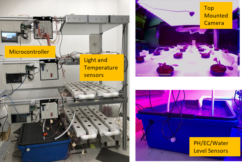
The experimental setup shown in Fig. 1 is housed in an air conditioned room where the temperature is kept at 25 ^∘deg Celsius. It consists of three levels of NFT hydroponics grow-bed, with the lighting conditions of each level individually controlled with a Raspberry Pi 3 micro-controller. The light source for each level is a dimmable panel with integrated red (650-670nm) and blue (450-465nm) LEDs mounted at 40cm above the grow-bed. Each grow-bed can support up to 20 lettuce plants, sharing the same nutrient solution with the other levels. The nutrient solution is circulated through the grow-beds with a pump from a 120 litre tank. The aim of the experiment is to collect information on how the lettuce plants will react to changes in lighting conditions. Hence, the values for nutrient concentration as well as the pH, as measured by the electro-conductivity (EC) sensor and pH sensor sourced from Atlas Scientific, are kept at consistent between 1600-2000 $\mu S/cm$ and $6.4-6.7$. Once the EC, pH, or water-level values dip below the desired threshold, a notification to top up the nutrient solution will be sent out by the micro-controller. Lighting, temperature and humidity conditions on each test bed are monitored by an array of sensors placed on each test bed. The raw values for the ISL29125 lux sensors used to monitor lighting were calibrated to the standard $\mu mol/m^{2}s$ units used to measure photosynthetic flux density (PPFD). Temperature and humidity under each were measured by DHT22 sensors. Data from the experimental setup are uploaded to a web server hourly. Prior to seeding of the lettuce plants, the power requirement of the LED panel at each red and blue PPFD settings were quantified in Watts using a power meter. The power requirements are shown in Fig. 2.

A top mounted camera is utilized to monitor the plant area throughout the course of each experiment in an attempt to quantify plant growth, as there is a strong correlation between plant leaf area and plant biomass [10]. Pictures on the growth of the plant were also sent to a web server hourly and the images batch-processed at the end of the experiment. However, it is a challenge for computers to recognize the leaf area for plants in an image. Leaf area segmentation techniques include simple thresholding like Otsu thresholding [11], to state of the art convolutional neural network (CNN) based approaches [12]. In our use case, simple thresholding does not work well with our images as they have too much variations in color, while CNN based techniques require too much effort to retrain the network for our setup. To avoid the time consuming task of manually labelling each image, we modified the K-means algorithm in [13] to come up with a helper algorithm in Algorithm 1 for plant segmentation.

In Fig. 3, under step 2 to step 3, we show the results of applying Algorithm 1 to images taken from day 3 to day 13 after the lettuce plants are transplants into the setup.

The relative growth rate (RGR) of a plant’s biomass typically follows an exponential relationship [15], as in Eq. 1.

where $M_{2}$ is the final dry mass, $M_{1}$ is the initial dry mass and $\triangle t$ is the change in time in days. In our experiment, we assumed that the increase in leaf area of a plant is related exponentially to a non-linear function that is dependent on the averaged light energy given to the plant over $\triangle t$, and external variables like EC and pH. The initial leaf area $L_{1}$ and final leaf area $L_{2}$ takes the place of $M_{1}$ and $M_{2}$, resulting in Eq. 2. $t$ is the time in days since transplanting.

A neural network is a universal function approximator [16], and will allow us to approximate the relationship between variables in Eq. 2. Data from the 4 experiments are split into testing and training data. Data from experiments 1,2,4 goes into the training set, while data from experiment 3 are used for testing. The design of the neural network, as well as the variables used are shown in Fig. 4. Variables are min-maxed to 0-1 according to the range displayed, again in Fig. 4. The neural network is a two layer feed forward network with ’relu’ neurons. Dropout of probability 0.5 is used for regularization to improve the accuracy of the network. The network was trained with back-propagation using the Adam optimizer with Mean Squared Error as the loss function for 2000 epochs.

A simple linear regression is also used to approximate $f(PPFD_{red_{avg}},PPFD_{blue_{avg}},EC,pH,t)$ for comparison with the neural network. The testing and training errors for both methods are summarized in Table II in terms of Mean Squared Error (MSE) and $R^{2}$ values to determine the goodness of fit of the model. The model is trained on the training data, and tested with either the training data or the testing data.

The neural network model performed much better than that of the linear regression by having a lower MSE and high $R^{2}$ value on both the training and testing datasets. However the difference in accuracy is lesser in the testing dataset as compared to the training dataset due to a slight distribution shift in the testing dataset.

Fig. 5 shows the shift in distribution and results of the eventual leaf area prediction. With more data, the neural network is expected to perform better than that of the linear regression, with its ability to model the non linear behaviour that may arise with lighting and plant growth interaction .

Once we have the plant model, we can track the sensitivity of the increase in leaf area to changes in lighting conditions. Eq. 2 can be manipulated as such to Eq. 3:

Assuming $EC=1800$, $pH=6.5$, and $\triangle t=1hr$, we investigated the increase in leaf area ($L_{2}-L_{1}$) when $t$= $1^{st}day$, $5^{th}day$, and $10^{th}day$ across the range of the light settings. The results are shown in Fig. 6.

The brighter portions of the heatmap in Fig. 6 denotes the lighting settings with higher growth rates. As we see, at the early stages of lettuce growth, the plant prefers a mixture of red and blue lighting for best growth. After some time, the preference of the plant switches over to red light. This is consistent in the findings in [17], who recommends mixing red and blue light in the ratio of 2.2:1 for lettuce growth, in the case of non adjustable LEDs. This ratio might not be the most cost effective option as blue leds will require more energy to provide the same irradiance level as red leds (Fig. 2). For LEDs with adjustable levels, we could leverage on the natural preference of the plant and adjust the lighting conditions for maximum growth and savings at each stage. For best growth on the 5th and 10th day, the ideal red to blue ratio is 14:1 and 20:1 respectively, as suggested by the plant model.

The optimization problem in Eq. 4 is a non-linear one due to the presence of non-linear constraints. Among the many other ways to solve non-linear optimization problems, Genetic Algorithm (GA) is reputed as a fast and efficient solver if the fitness function can be quickly evaluated, making it a great algorithm to solve Eq. 4. The first step in a genetic algorithm is to represent the solution of the problem in a chromosome. For our optimization problem, the chromosome is a 360 long vector with each bin taken up by a tuple, $(r_{\delta},b_{\delta})$. Both $(r_{\delta},b_{\delta})\in Z:\{1...10\}$, with 1 representing 10% of maximum PPFD and 10 representing 100% of max PPFD. The maximum PPFD for red LEDs in our system is 200 $\mu mol/m^{2}s$, while for the blue LEDs it is at 100 $\mu mol/m^{2}s$. A $(r_{\delta}=3,b_{\delta}=3)$ tuple will mean that the red LEDs are outputting PPFD at 60 $\mu mol/m^{2}s$ while the blue LEDs are outputting at 30 $\mu mol/m^{2}s$. The fitness function is the objective function in Eq. 4. Beyond that, the steps in GA like population generation, crossover, and mutation follows that of the canonical version stated in [19]. Parameters relevant to GA are listed in Table IV.

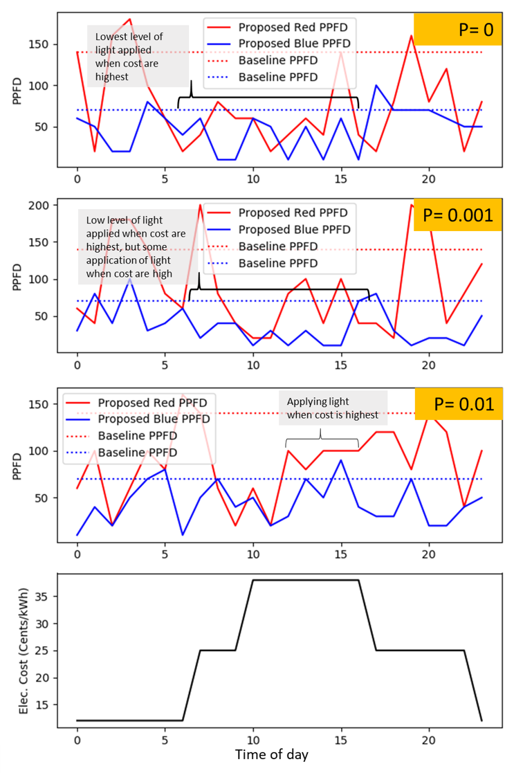
Different values of $P$ were tested, $P$ = 0, $P$ = 0.001, and $P$ = 0.01. The generated control sequences from GA were also compared to a $(r_{\delta}=7,b_{\delta}=7)$ 24hr always-on baseline sequence, as recommended by [17].

Fig. 7 shows the convergence of the fitness function in various cases of $P$.

When $P$ = 0, the fitness function is dominated by the cost of electricity over the period of 15 days. Hence, this will lead to the control sequences being optimized for a low electricity cost, subjected to constraint that the final leaf area of the plant must be more than 400 $cm^{2}$. When $P$ is low at 0.001, the revenue from selling the plant will be approximately equal to the cost of electricity, this will induce the GA to search for control sequences that balances the cost of electricity with the final leaf area. Finally when $P$ is high at 0.01, the GA will tend to search for control sequence that favor a larger final leaf area over lowering the cost of electricity.

The control sequence for the $1^{st}$ 24 hour sequence in $s$ for various $P$ values are shown in Fig. 8. We see that when the $P$ is highest, the GA optimizes the growth of the plant by offering more light even when the cost of electricity is high. When $P$ is the lowest, the GA choose to only operate the lights at the portion when electricity prices are the lowest. For $P$ = 0.001, the GA balances the growth of the plant with the cost of electricity.

The final leaf area and electricity cost are summarized in the Table. V. Profit is the objective function of the problem defined in Eq. 4. When compared to the baseline, the GA allows the system to achieve between 40-52% savings in electricity cost. Meanwhile, the leaf area output can be improve by up to 6%.