Dirac/Rarita-Schwinger plus Maxwell theories in $\mathbb{R}\times S^{3}$ spacetime in the Hopf coordinates

We consider Dirac-Maxwell theory, where the source of electromagnetic field is taken in the form of a massless Dirac field. The corresponding Lagrangian can be written as (hereafter, we work in units where $\hbar=c=1$)

which contains the covariant derivative $\psi_{;\mu}\equiv\left[\partial_{\mu}+1/8\,\omega_{ab\mu}\left(\gamma^{a}\gamma^{b}-\gamma^{b}\gamma^{a}\right)-ieA_{\mu}\right]\psi$, where $\gamma^{a}$ are the Dirac matrices in flat space (below we use the spinor representation of the matrices); $a,b$ and $\mu,\nu$ are tetrad and spacetime indices, respectively; $F_{\mu\nu}=\partial_{\mu}A_{\nu}-\partial_{\nu}A_{\mu}$ is the electromagnetic field tensor; $A_{\mu}$ are four-potentials of the electromagnetic field; $e$ is a charge in Maxwell theory. In turn, the Dirac matrices in curved space, $\gamma^{\mu}=e_{a}^{\phantom{a}\mu}\gamma^{a}$, are obtained using the tetrad $e_{a}^{\phantom{a}\mu}$, and $\omega_{ab\mu}$ is the spin connection [for its definition, see Ref. Lawrie2002, formula (7.135)].

Varying the corresponding action with the Lagrangian (1), one can obtain the following set of equations:

where $g$ is the determinant of the metric tensor and $j^{\mu}=e\bar{\psi}\gamma^{\mu}\psi$ is the four-current.

We seek a solution of the above equations in $\mathbb{R}\times S^{3}$ spacetime with the Hopf coordinates $\chi,\theta,\varphi$ on a sphere $S^{3}$. The corresponding metric is

where $dS^{2}_{3}$ is the Hopf metric on the unit $S^{3}$ sphere; $r$ is a constant; $0\leq\chi,\varphi\leq 2\pi$ and $0\leq\theta\leq\pi$. For a detailed description of the Hopf fibration, see Appendix A.

To solve Eqs. (2) and (3), we use the following $\mathfrak{Ansatz}$ for the spinor and electromagnetic fields:

where $m,n$ are integers. The spinor may transform under a rotation through an angle $2\pi$ as

Then, due to the presence of the factors $e^{in\chi}$ and $e^{im\varphi}$ in Eq. (5), the spinors $\psi_{mn}$ and $\psi_{pq}$ with different pairs of indices $(m,n)$ and $(p,q)$ are orthogonal.

To solve the equations, we employ the tetrad

coming from the metric (4). Taking all this into account, the current $j^{\mu}$ [for its definition, see after Eq. (3)] is

After substitution of the $\mathfrak{Ansatz}$ (5) and (6) in Eqs. (2) and (3), we have

where the prime denotes differentiation with respect to $\theta$. Note that the set of equations (7)-(11) must be solved as an eigenvalue problem for $\Omega$ with the eigenfunctions $\Theta_{1,2}$.

We seek a solution in the following particular form:

and the eigenparameter $\Omega$ is given by the expression

It is seen from this expression that the energy of the system $\Omega$ depends on $n$ only, i.e., the energy spectrum is degenerate with respect to $m$.

For the above particular solution, Eq. (11) is satisfied identically, and the remaining equations yield the set of equations for the functions $\Theta,\phi,\rho$, and $\lambda$,

where we have introduced new dimensionless variables $\tilde{\rho},\tilde{\lambda},\tilde{\phi}=er\left(\rho,\lambda,\phi\right)$ and $\tilde{\Theta}=er^{3/2}\Theta$. From the Maxwell equations (14) and (15), it then follows that $\tilde{\phi}=\mp 2\tilde{\rho}$.

Before solving the full set of equations (13)-(16), consider the case of “frozen” electric and magnetic fields, where the scalar and vector potentials $\phi=\rho=\lambda=0$. The solution of Eq. (13) is then Dzhunushaliev:2020dom

Here, we explicitly take the integration constant in the form $C/r^{3/2}$ so that the constant $C$ would be dimensionless.

Since the spinors $\psi_{mn}$ and $\psi_{pq}$ are orthogonal for $(m,n)\neq(p,q)$, using the normalization condition

one can find the normalization constant

The condition of the positiveness of the $\Gamma$ functions leads to the following inequalities for the quantum numbers $m$ and $n$:

In this case, the solution energy spectrum (12) satisfies the inequalities

Consider now some physical properties of the solution (17). The spin density tensor for the Dirac field is defined as

where $\sigma_{ab}=(i/2)\left[\gamma_{a},\gamma_{b}\right]$. After substituting the $\mathfrak{Ansatz}$ (5), we have the following nonzero components of this tensor:

where $\mathcal{A}=\Theta_{1}^{2}+\Theta^{2}_{2},\mathcal{C}=\Theta_{1}\Theta_{2},\mathcal{D}=\Theta_{1}^{2}-\Theta^{2}_{2}$. After substituting the solution (17), we get the absolutely antisymmetric tensor

The current $j^{a}$ is defined as

and for the exact solution (17) it is

with the 1-forms $\omega^{0}=dt,\;\omega^{1}=d\chi-\cos\theta d\varphi.$

The 1-form $\omega^{1}$ defines the Hopf invariant (see Appendix A)

The energy-momentum tensor is

where $\mathcal{B}=\left(\Theta_{1}+\Theta_{2}\right)^{2}$ and $\mathcal{E}=\Theta_{1}^{\prime}\Theta_{2}-\Theta_{2}^{\prime}\Theta_{1}$. For the solution (17), we have

Since Eqs. (13)-(16) cannot be integrated analytically, we will seek their numerical solution. Before doing that, it is necessary to find an approximate solution near the point $\theta=0$, which may be sought in the form of the following power series:

where $\alpha,\gamma,\delta,\epsilon,a_{i},f_{i},c_{i},d_{i}$ are parameters to be determined. Substituting (19) in Eqs. (13)-(16) and comparing the leading terms, we find the values of the expansion parameters

Thus, for numerical computations, we have the following values of the functions at the point $\theta=\Delta$:

where the parameter $a_{0}$ is arbitrary. Since the functions $\tilde{\rho}$ and $\tilde{\phi}$ are linearly proportional [see the corresponding expression after Eq. (16)], for $\tilde{\phi}$, there will be an expansion similar to that given above for $\tilde{\rho}$. Also, since the set of equations (13)-(16) contains $\sin\theta$ in the denominator, we start the numerical solution not from the point $\theta=0$ but from $\theta=\Delta\ll 1$.

In the case under consideration, the components of the electric, $E_{\theta}$, and magnetic, $H_{\chi,\varphi}$, fields are

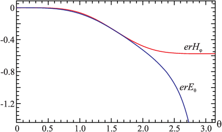
The results of calculations are given in Figs. 2 and 2 [note that for plotting these graphs we have chosen the upper signs in Eqs. (13) and (15)]. The analysis of this numerical solution indicates that the function $\Theta$ is practically coincide with the analytic solution (17) obtained in the absence of the fields $\phi,\lambda$, and $\rho$. In turn, using the solutions found, one can also calculate the energy-momentum tensor (18).

Consider the theory describing the interaction of the Rarita-Schwinger field $\psi_{ai}$ with a Maxwellian electromagnetic field. The Maxwell equations keep their form (3), and the Rarita-Schwinger equations describing massless spin-3/2 particles are

Here, the covariant derivative $\nabla_{\mu}\psi_{ai}=\partial_{\mu}\psi_{ai}+\frac{1}{4}\omega_{bc\mu}\gamma^{b}_{ij}\gamma^{c}_{jk}\psi_{ak}-\omega^{b}_{\phantom{b}a\mu}\psi_{bi}-ieA_{\mu}\psi_{ai}$ involves the spinor, $i,j,k$, tetrad, $a,b,c$, and spacetime, $\mu$, indices, the four-current $j^{\mu}=\epsilon^{abcd}\bar{\psi}_{ai}\left(\gamma_{5}\right)_{ij}\left(\gamma_{b}\right)_{jk}e^{\mu}_{c}\psi_{dk}$ with $\epsilon^{abcd}$ being the completely antisymmetric Levi-Civita symbol.

The spinor Rarita-Schwinger field must also satisfy the following constraints Redkov:2011ttu (hereafter, we drop the spinor index $i$ in $\psi_{ai}$ for simplicity):

where $\kappa$ is a numerical coefficient, $F_{ab}$ is the electromagnetic field tensor with tetrad indices, $R_{ab}$ and $R$ are the Ricci tensor and the scalar curvature, respectively. Taking into account the constraints (21) and (22), Eq. (20) can be recast in the following equivalent form:

where $\nabla_{\mu}\psi_{\nu}=e^{a}_{\phantom{a}\nu}\nabla_{\mu}\psi_{a}$; in this form, it is used in SUGRA.

One of distinctive features of the Rarita-Schwinger equation is that the spinor $\psi_{a}$ has 16 components, but the constraints (21) and (22) reduce the number of independent components to 8. This means that this equation is overconstrained, and the derivation of its solutions is hampered by this fact.

In this case, there is only the Rarita-Schwinger equation (20) with the constraints (21) and (22). Since we consider the case of a massless spinor field, we will seek a solution of Eq. (20) in $\mathbb{R}\times S^{3}$ spacetime with the metric (4) in the form

Here, we have split the Rarita-Schwinger spinor $\left(\psi_{a}\right)_{mn}$ into two Weyl spinors, one of which is set to be zero: $\left(\chi_{a}\right)_{mn}=0$. The integers $m$ and $n$ appearing here are quantum numbers, and $(\dots)^{T}$ denotes the transpose for the spinor indices but not for the tetrad index $a$.

After substitution of the $\mathfrak{Ansatz}$ (24) in Eq. (20), we get the following set of equations:

Let us now assume that the left-hand and right-hand sides of the constraint equation (21) are equal to zero separately [below we will show that this assumption is valid for the solutions obtained, see after Eq. (40)]. This leads to the constraint $\gamma^{a}\psi_{a}=0$, from which the following relations between the components of the spinor are found to be

After substitution of (31) in Eqs. (25)-(30), one can eliminate $\Theta_{23}^{\prime},\Theta_{33}^{\prime},\Theta_{24}^{\prime},\Theta_{34}^{\prime}$ from Eqs. (27) and (30) and get the following relations between the components of the spinor:

Substituting this in the initial set of equations, we find the following equations for the $\Theta_{23}$ and $\Theta_{24}$ components of the spinor:

where the eigenvalue $\Omega_{n}$ is defined as

As in the case of the Dirac field [see after Eq. (12)], one can see from this expression that, since the energy of the system $\Omega$ depends on $n$ only, the energy spectrum is degenerate with respect to $m$.

We seek a solution of the above equations in the particular form

obtaining the equation

Taking into account the expressions (31)-(33), we then have the following set of solutions:

References

• (1) W. Greiner, Relativistic quantum mechanics: Wave equations (Springer-Verlag, Berlin, New York, 2000).
• (2) S. Chandrasekhar, The Mathematical Theory of Black Holes (Oxford University Press, New York, 1983).
• (3) S. W. Goatham and S. Krusch, “Fermions, Skyrmions and the 3-Sphere,” J. Phys. A 43, 035402 (2010).
• (4) R. Gueven, “Black holes have no superhair,” Phys. Rev. D 22, 2327 (1980).
• (5) R. Gueven, “Extreme Reissner-Nordstrom black holes can support a ’superhair’,” Phys. Rev. D 25, 3117 (1982).
• (6) G. F. Torres del Castillo and G. Silva-Ortigoza, “Rarita-Schwinger fields in the Kerr geometry,” Phys. Rev. D 42, 4082 (1990).
• (7) F. Anton and E. Porter-Hope, “Spin-3/2 massless field in a Kerr-Newman background metric,” Phys. Rev. D 38, 3318 (1988).
• (8) A. Szereszewski and J. Tafel, “Solutions of the Rarita-Schwinger equation in Einstein spaces,” Phys. Lett. A 297, 359 (2002).
• (9) T. Pilling, “Symmetry of massive Rarita-Schwinger fields,” Int. J. Mod. Phys. A 20, 2715 (2005).
• (10) G. Velo and D. Zwanziger, “Propagation and quantization of Rarita-Schwinger waves in an external electromagnetic potential,” Phys. Rev. 186, 1337 (1969).
• (11) Y. Pang and J. Rong, “N=3 solution in dyonic ISO(7) gauged maximal supergravity and its uplift to massive type IIA supergravity,” Phys. Rev. D 92, 085037 (2015).
• (12) B. Hoare and A. A. Tseytlin, “Type IIB supergravity solution for the T-dual of the η\eta-deformed AdS5×{}_{5}\times S5 superstring,” JHEP 10, 060 (2015).
• (13) G. W. Gibbons, C. N. Pope, and E. Sezgin, “The General Supersymmetric Solution of Topologically Massive Supergravity,” Class. Quant. Grav. 25, 205005 (2008).
• (14) I. Lawrie, A unified grand tour of theoretical physics (Institute of Physics Publishing, Bristol and Philadelphia, 2002).
• (15) V. Dzhunushaliev and V. Folomeev, “Spinor field solutions in F⁡(B2)F\left(B^{2}\right) modified Weyl gravity,” [arXiv:2003.02646 [gr-qc]].
• (16) V. M. Red’kov, “Particle with spin S=3/2 in Riemannian space-time,” arXiv:1109.3871 [math-ph].