跳到论文正文
W Papers独立论文阅读器 arXiv:2008.01006 论文正文 计算阅读时间 · 0%
引用这篇论文根据当前论文元数据生成,正式投稿前建议核对。


License: arXiv.org perpetual non-exclusive license
arXiv:2008.01006v7 [math.ST] 02 May 2021

Gibbs sampler and coordinate ascent variational inference: A set-theoretical review

Se Yoon Lee Affiliation: Department of Statistics, Texas A&M University, College Station, Texas, USA Email: seyoonlee@stat.tamu.edu
Abstract

One of the fundamental problems in Bayesian statistics is the approximation of the posterior distribution. Gibbs sampler and coordinate ascent variational inference are renownedly utilized approximation techniques that rely on stochastic and deterministic approximations. In this paper, we define fundamental sets of densities frequently used in Bayesian inference. We shall be concerned with the clarification of the two schemes from the set-theoretical point of view. This new way provides an alternative mechanism for analyzing the two schemes endowed with pedagogical insights.

Keywords: Gibbs sampler; Coordinate ascent variational inference; Duality formula.

1 Introduction

A statistical model contains a sample space of observations y endowed with an appropriate σ\sigma-field of sets over which is given a family of probability measures. For almost all problems, it is sufficient to suppose that these probability measures can be described through their density functions, p⁡(y|𝜽)p(\textbf{y}|\bm{\theta}), indexed by a parameter 𝜽\bm{\theta} belonging to the parameter space 𝚯\bm{\Theta}. In many problems, one of the essential goals is to make an inference about the parameter 𝜽\bm{\theta}, and this article particularly concerns Bayesian inference.

Bayesian approaches start with expressing the uncertainty associated with the parameter 𝜽\bm{\theta} through a density π⁡(𝜽)\pi(\bm{\theta}) supported on the parameter space 𝚯\bm{\Theta}, called a prior. A collection {p⁡(y|𝜽),π⁡(𝜽)}\{p(\textbf{y}|\bm{\theta}),\pi(\bm{\theta})\} is referred to as a Bayesian model. Given finite evidence m⁡(y)=∫p⁡(y|𝜽)⋅π⁡(𝜽)​𝑑𝜽m(\textbf{y})=\int p(\textbf{y}|\bm{\theta})\cdot\pi(\bm{\theta})d\bm{\theta} for all y, the Bayes’ theorem formalizes an inversion process to learn the parameter 𝜽\bm{\theta} given the observations y through its posterior distribution:

π⁡(𝜽|y)=p⁡(y|𝜽)⋅π⁡(𝜽)m⁡(y).\displaystyle\pi(\bm{\theta}|\textbf{y})=\frac{p(\textbf{y}|\bm{\theta})\cdot\pi(\bm{\theta})}{m(\textbf{y})}. (1)

A central task in the application of Bayesian models is the evaluation of this joint density π⁡(𝜽|y)\pi(\bm{\theta}|\textbf{y}) (1) or indeed to compute expectation with respect to this density.

However, for many complex Bayesian models, the posterior distribution π⁡(𝜽|y)\pi(\bm{\theta}|\textbf{y}) is intractable. In such situations, we need to resort to approximation techniques, and these fall broadly into two classes, according to whether they rely on stochastic (Casella and George 1992; Neal et al. 2011; Murray et al. 2010; Neal 2003) or deterministic (Ranganath et al. 2014; Wang and Blei 2013; Minka 2013; Blei et al. 2017) approximations. See (Andrieu et al. 2003; Zhang et al. 2018) for review papers for these techniques.

Gibbs sampler (Casella and George 1992) and coordinate ascent variational inference (CAVI) algorithm (Blei et al. 2017) are extremely popular techniques to approximate the target density π⁡(𝜽|y)\pi(\bm{\theta}|\textbf{y}) (1). They are often jointed with more sophisticated samplers or optimizers, and share some common structure from an implementational point of view. For instances, Gibbs sampler is combined with the Metropolis-Hastings algorithms (Chib and Greenberg 1995; Beichl and Sullivan 2000; Dwivedi et al. 2018) endowed with a nice proposal density which is typically easy to simulate from. The CAVI algorithm is combined with the stochastic gradient descent method (Ruder 2016) endowed with a reasonable assumption of mean-field family whose members are computationally tractable.

Essentially, the utilities of the two schemes are ascribed to their exploitations of the conditional independences (Dawid 1979) induced by a certain hierarchical structure formulated through the parameter 𝜽\bm{\theta} and observations y. That way, we can decompose the original problem of approximation of the joint density π⁡(𝜽|y)\pi(\bm{\theta}|\textbf{y}), possibly supported on a high-dimensional parameter space 𝚯\bm{\Theta}, into a collection of small problems with low dimensionalities. A single cycle of resulting algorithms comprises multiple steps where at each step only a small fraction of the 𝜽\bm{\theta} is updated, while remaining components are fixed with the most recently updated information.

This article aims to understand the two schemes set-theoretically to clarify some common structure between the two schemes and provide relevant pedagogical insights. Here, we say “set-theoretical understanding” in the sense that we will treat fundamental densities used in the two schemes as elements of some sets of densities. Set-theoretical statements are helpful in a clear understanding of the algorithms as they explain how ingredients of the two schemes are functionally related each other. A duality formula for variational inference (Massart 2007) is the essential theorem for the expositions.

2 A duality formula for variational inference

To state a duality formula for variational inference, we first introduce some ingredients. Let 𝚯\bm{\Theta} be a set endowed with an appropriate σ\sigma-field ℱ\mathcal{F}, and two probability measures PP and QQ, which formulates two probability spaces, (𝚯,ℱ,P)(\bm{\Theta},\mathcal{F},P) and (𝚯,ℱ,Q)(\bm{\Theta},\mathcal{F},Q). We use notation Q≪PQ\ll P to indicate that QQ is absolutely continuous with respect to PP (i.e., Q⁡(A)=0Q(A)=0 holds for any measurable set A∈ℱA\in\mathcal{F} with P⁡(A)=0P(A)=0). Let 𝔼P​[⋅]\mathbb{E}_{P}[\cdot] denote integration with respect to the probability measure PP. Given any real-valued random variable gg defined on the probability space (𝚯,ℱ,P)(\bm{\Theta},\mathcal{F},P), notation g∈L1​(P)g\in L_{1}(P) implies that the random variable gg is integrable with respect to measure PP, that is, 𝔼P​[|g|]=∫|g|​𝑑P<∞\mathbb{E}_{P}[|g|]=\int|g|dP<\infty. The notation KL(Q∥P)\text{KL}(Q\|P) represents the Kullback-Leibler divergence from PP to QQ, KL(Q∥P)=∫log(dQ/dP)dQ\text{KL}(Q\|P)=\int\log\ (dQ/dP)dQ (Kullback 1997).

Theorem 2.1 (Duality formula).

Consider two probability spaces (𝚯,ℱ,P)(\bm{\Theta},\mathcal{F},P) and (𝚯,ℱ,Q)(\bm{\Theta},\mathcal{F},Q) with Q≪PQ\ll P. Assume that there is a common dominating probability measure λ\lambda such that P≪λP\ll\lambda and Q≪λQ\ll\lambda. Let hh denote any real-valued random variable on (𝚯,ℱ,P)(\bm{\Theta},\mathcal{F},P) that satisfies exp⁡h∈L1​(P)\exp h\in L_{1}(P). Then the following equality holds

log⁡𝔼P​[exp⁡h]\displaystyle\log\mathbb{E}_{P}[\exp h] =supQ≪P{𝔼Q[h]−KL(Q∥P)}.\displaystyle=\text{sup}_{Q\ll P}\{\mathbb{E}_{Q}[h]-\text{KL}(Q\|P)\}.

Further, the supremum on the right-hand side is attained if and only if it holds

q⁡(θ)p⁡(θ)=exp⁡h⁡(θ)𝔼P​[exp⁡h],\displaystyle\frac{q(\theta)}{p(\theta)}=\frac{\exp h(\theta)}{\mathbb{E}_{P}[\exp h]},

almost surely with respect to probability measure QQ, where p⁡(θ)=d​P/d​λp(\theta)=dP/d\lambda and q⁡(θ)=d​Q/d​λq(\theta)=dQ/d\lambda denote the Radon-Nikodym derivatives of the probability measures PP and QQ with respect to λ\lambda, respectively.

Proof.

We use a measurement theory (Royden and Fitzpatrick 1988) for a direct proof. Due to the dominating assumptions P≪λP\ll\lambda and Q≪λQ\ll\lambda and the Radon-Nikodym theorem (Theorem 32.1 of (Billingsley 2008)), there exist Radon-Nikodym derivatives (also called generalized probability densities (Kullback 1997)) p⁡(θ)=d​P/d​λp(\theta)=dP/d\lambda and q⁡(θ)=d​Q/d​λq(\theta)=dQ/d\lambda unique up to sets of measure (probability) zero in λ\lambda corresponding to measures PP and QQ, respectively. On the other hand, due to the dominating assumption Q≪PQ\ll P, there exists Radon-Nikodym derivative d​Q/d​PdQ/dP, hence, Kullback-Leibler divergence KL(Q∥P)=∫log(dQ/dP)dQ\text{KL}(Q\|P)=\int\log\ (dQ/dP)dQ is well-defined and finite. By using conventional measure-theoretic notation (for example, see page 4 of (Kullback 1997)), we shall write d​P​(θ)=p⁡(θ)​d​λ​(θ)dP(\theta)=p(\theta)d\lambda(\theta) and d​Q​(θ)=q⁡(θ)​d​λ​(θ)dQ(\theta)=q(\theta)d\lambda(\theta), and ∫g​𝑑P=∫g⁡(θ)​𝑑P​(θ)\int gdP=\int g(\theta)dP(\theta) for any g∈L1​(P)g\in L_{1}(P) (Resnick 2003).

Use the measure theoretic ingredients as follow:

𝔼Q[h]−KL(Q∥P)\displaystyle\mathbb{E}_{Q}[h]-\text{KL}(Q\|P) =∫h​𝑑Q−∫log⁡(d​Qd​P)​𝑑Q\displaystyle=\int hdQ-\int\log\ \bigg(\frac{dQ}{dP}\bigg)dQ
=∫h⁡(θ)​𝑑Q​(θ)−∫log⁡(d​Q​(θ)d​P​(θ))​𝑑Q​(θ)\displaystyle=\int h(\theta)dQ(\theta)-\int\log\ \bigg(\frac{dQ(\theta)}{dP(\theta)}\bigg)dQ(\theta)
=∫h⁡(θ)​q​(θ)​𝑑λ​(θ)−∫log⁡(q⁡(θ)p⁡(θ))​q​(θ)​𝑑λ​(θ)\displaystyle=\int h(\theta)q(\theta)d\lambda(\theta)-\int\log\ \bigg(\frac{q(\theta)}{p(\theta)}\bigg)q(\theta)d\lambda(\theta)
=∫log⁡(eh⁡(θ)​p​(θ)q⁡(θ))​q​(θ)​𝑑λ​(θ)\displaystyle=\int\log\ \bigg(\frac{e^{h(\theta)}p(\theta)}{q(\theta)}\bigg)q(\theta)d\lambda(\theta)
≤log⁡(∫(eh⁡(θ)​p​(θ)q⁡(θ))​q​(θ)​𝑑λ​(θ))\displaystyle\leq\log\bigg(\int\bigg(\frac{e^{h(\theta)}p(\theta)}{q(\theta)}\bigg)q(\theta)d\lambda(\theta)\bigg) (2)
=log⁡(∫eh⁡(θ)​p​(θ)​𝑑λ​(θ))\displaystyle=\log\bigg(\int e^{h(\theta)}p(\theta)d\lambda(\theta)\bigg)
=log⁡(∫eh⁡(θ)​𝑑P​(θ))\displaystyle=\log\bigg(\int e^{h(\theta)}dP(\theta)\bigg)
=log⁡(∫eh​𝑑P)\displaystyle=\log\bigg(\int e^{h}dP\bigg)
=log⁡𝔼P​[exp⁡h].\displaystyle=\log\mathbb{E}_{P}[\exp h].

Note that the Jensen’s inequality is used to derive the inequality in (2). Because the logarithm function is strictly concave, this inequality becomes the equality if and only if the function eh⁡(θ)​p​(θ)/q⁡(θ)e^{h(\theta)}p(\theta)/q(\theta) is constant on 𝚯\bm{\Theta} almost surely with respect to measure QQ (page 52 of (Keener 2010)). Let eh⁡(θ)​p​(θ)/q⁡(θ)=ke^{h(\theta)}p(\theta)/q(\theta)=k, where kk is constant almost surely with respect to QQ. Then we have eh⁡(θ)​p​(θ)=k​q​(θ)e^{h(\theta)}p(\theta)=kq(\theta). Take the integral ∫⋅dλ(θ)\int\cdot d\lambda(\theta) on both sides on the final equation to complete the proof: 𝔼P​[exp⁡h]=∫eh​𝑑P=∫eh⁡(θ)​𝑑P​(θ)=∫eh⁡(θ)​p​(θ)​𝑑λ​(θ)=∫k​q​(θ)​𝑑λ​(θ)=∫k​𝑑Q​(θ)=∫k​𝑑Q=k\mathbb{E}_{P}[\exp h]=\int e^{h}dP=\int e^{h(\theta)}dP(\theta)=\int e^{h(\theta)}p(\theta)d\lambda(\theta)=\int kq(\theta)d\lambda(\theta)=\int kdQ(\theta)=\int kdQ=k. ∎

In practice, a common dominating measure λ\lambda for PP and QQ is usually either Lebesgue or counting measure. This article mainly explores the former case where the duality formula becomes

log⁡𝔼p⁡(θ)​[exp⁡h⁡(θ)]\displaystyle\log\mathbb{E}_{p(\theta)}[\exp h(\theta)] =supq≪p{𝔼q⁡(θ)[h(θ)]−KL(q∥p)}.\displaystyle=\text{sup}_{q\ll p}\{\mathbb{E}_{q(\theta)}[h(\theta)]-\text{KL}(q\|p)\}. (3)

In equality (3), the p⁡(θ)=d​P/d​λp(\theta)=dP/d\lambda and q⁡(θ)=d​Q/d​λq(\theta)=dQ/d\lambda are probability density functions (pdf) corresponding to the probability measures PP and QQ, respectively, and h⁡(θ)h(\theta) is any measurable function such that the expectation 𝔼p⁡(θ)​[exp⁡h​(θ)]\mathbb{E}_{p(\theta)}[\exp h(\theta)] is finite. Expectations in the equilibrium (3) are taken with respect to densities on the subscripts. For instance, the expectation 𝔼p⁡(θ)​[exp⁡h​(θ)]\mathbb{E}_{p(\theta)}[\exp h(\theta)] represents the integral ∫exp⁡h⁡(θ)​p​(θ)​𝑑θ\int\exp h(\theta)p(\theta)d\theta, and the Kullback-Leibler divergence is expressed with the pdf version, that is, KL(q(θ)∥p(θ))=∫q(θ)log(q(θ)/p(θ))dθ\text{KL}(q(\theta)\|p(\theta))=\int q(\theta)\log(q(\theta)/p(\theta))d\theta. We shall use the notation q≪pq\ll p to indicate that their corresponding probability measures satisfy the dominating condition Q≪PQ\ll P.

3 Fundamental sets in Bayesian inference

Consider a Bayesian model {p⁡(y|𝜽),π⁡(𝜽)}\{p(\textbf{y}|\bm{\theta}),\pi(\bm{\theta})\} where p⁡(y|𝜽)p(\textbf{y}|\bm{\theta}) is a data generating process and π⁡(𝜽)\pi(\bm{\theta}) is a prior density as explained in Section 1. Now, we additionally assume that the entire parameter space 𝚯\bm{\Theta} is decomposed as

𝚯=Πi=1KΘi=Θ1×⋯×Θi×⋯×ΘK,\displaystyle\bm{\Theta}=\Pi_{i=1}^{K}\Theta_{i}=\Theta_{1}\times\cdots\times\Theta_{i}\times\cdots\times\Theta_{K}, (4)

for some integer K>1K>1. Each component parameter space Θi\Theta_{i} (i=1,⋯,Ki=1,\cdots,K) can be a set of scalar components, subvectors, or matrices (Smith and Roberts 1993). The notation A×BA\times B denotes the Caresian product between two sets AA and BB. Under the decomposition (4), elements of the set 𝚯\bm{\Theta} can be expressed as 𝜽=(θ1,⋯,θi,⋯,θK)∈𝚯\bm{\theta}=(\theta_{1},\cdots,\theta_{i},\cdots,\theta_{K})\in\bm{\Theta} where θi∈Θi\theta_{i}\in\Theta_{i} (i=1,⋯,Ki=1,\cdots,K).

For each ii, we define a set that complements the ii-th component parameter space Θi\Theta_{i}:

Θ−i:=Πj=1,j≠iKΘj=Θ1×⋯×Θi−1×Θi+1×⋯×ΘK.\displaystyle\Theta_{-i}\vcentcolon=\Pi_{j=1,j\neq i}^{K}\Theta_{j}=\Theta_{1}\times\cdots\times\Theta_{i-1}\times\Theta_{i+1}\times\cdots\times\Theta_{K}. (5)

The set Θ−i\Theta_{-i} (5) is called the ii-th complementary parameter space. Elements of the Θ−i\Theta_{-i} are of the form θ−i=(θ1,⋯,θi−1,θi+1,⋯,θK)∈Θ−i\theta_{-i}=(\theta_{1},\cdots,\theta_{i-1},\theta_{i+1},\cdots,\theta_{K})\in\Theta_{-i}.

Refer to caption
Figure 1: Venn diagram that superimposed two set-inclusion relationships: (1) 𝒬𝜽|yM​F⊂𝒬𝜽|y⊂𝒬𝜽\mathcal{Q}_{\bm{\theta}|\textbf{y}}^{MF}\subset\mathcal{Q}_{\bm{\theta}|\textbf{y}}\subset\mathcal{Q}_{\bm{\theta}}, and (2) 𝒬θi|ym⊂𝒬θi|y⊂𝒬θi\mathcal{Q}_{\theta_{i}|\textbf{y}}^{m}\subset\mathcal{Q}_{\theta_{i}|\textbf{y}}\subset\mathcal{Q}_{\theta_{i}} for each component index ii (i=1,⋯,Ki=1,\cdots,K). Symbol ∙\bullet indicates an element of the sets. For each ii, π⁡(θi|θ−i,y)\pi(\theta_{i}|\theta_{-i},\textbf{y}) (10), π⁡(θi|y)\pi(\theta_{i}|\textbf{y}), and q∗​(θi)q^{*}(\theta_{i}) (14) are the full conditional, marginal posterior, and variational factor, respectively. The π⁡(𝜽)\pi(\bm{\theta}), π⁡(𝜽|y)\pi(\bm{\theta}|\textbf{y}) (1), and q∗​(𝜽)q^{*}(\bm{\theta}) are prior density, posterior density, and VB posterior, respectively.

It is important to emphasize that how to impose a decomposition on the set 𝚯\bm{\Theta} (i.e., to determine the integer KK or the dimension of the component parameter spaces Θi\Theta_{i} in (4)) is at the discretion of a model builder. Although it is possible to fully factorize the 𝚯\bm{\Theta} so that every Θi\Theta_{i} consists of scalar components, sampling or optimization algorithm based on such a decomposition may have limited accuracy, especially when the latent variables are highly dependent. One important consideration in choosing a decomposition (4) is the correlation structure embedded in the target density π⁡(𝜽|y)\pi(\bm{\theta}|\textbf{y}). For instance, when a Bayesian model {p⁡(y|𝜽),π⁡(𝜽)}\{p(\textbf{y}|\bm{\theta}),\pi(\bm{\theta})\} formulates a certain hierarchical structure, one can impose a decomposition based on the conditional independence induced by the hierarchy among the latent variables θi\theta_{i}’s and observations y, thereby exploiting the notion of Markov blankets (Pellet and Elisseeff 2008).

Now, we define fundamental sets of densities, itemized with (i) – (vi). They play crucial roles in Bayesian inference about the parameter 𝜽\bm{\theta} provided that Gibbs sampler or CAVI algorithm is carried out to approximate the target density π⁡(𝜽|y)\pi(\bm{\theta}|\textbf{y}) (1):

  • (i)

    Set 𝒬𝜽\mathcal{Q}_{\bm{\theta}} is the collection of all the densities supported on the parameter space 𝚯\bm{\Theta}. Thus, the 𝒬𝜽\mathcal{Q}_{\bm{\theta}} is the largest set of densities that we can consider in Bayesian inference. Set 𝒬𝜽|y\mathcal{Q}_{\bm{\theta}|\textbf{y}} is the collection of all the densities conditioned on the observations y. Here, the term ‘conditioned on the observations y’ can be also replaced by term ‘having observed y’, or more concisely by ‘a posteriori’. By definitions, it holds a subset inclusion, 𝒬𝜽|y⊂𝒬𝜽\mathcal{Q}_{\bm{\theta}|\textbf{y}}\subset\mathcal{Q}_{\bm{\theta}}. Both prior and posterior densities, π⁡(𝜽)\pi(\bm{\theta}) and π⁡(𝜽|y)\pi(\bm{\theta}|\textbf{y}) (1), belong to the set 𝒬𝜽\mathcal{Q}_{\bm{\theta}}. And in particular, the posterior density π⁡(𝜽|y)\pi(\bm{\theta}|\textbf{y}) belongs to the set 𝒬𝜽|y\mathcal{Q}_{\bm{\theta}|\textbf{y}}. As the prior density π⁡(𝜽)\pi(\bm{\theta}) does not involve the observations y, it holds π⁡(𝜽)∈𝒬𝜽−𝒬𝜽|y=𝒬𝜽∩(𝒬𝜽|y)c\pi(\bm{\theta})\in\mathcal{Q}_{\bm{\theta}}-\mathcal{Q}_{\bm{\theta}|\textbf{y}}=\mathcal{Q}_{\bm{\theta}}\cap(\mathcal{Q}_{\bm{\theta}|\textbf{y}})^{c};

  • (ii)

    For each ii (i=1,⋯,Ki=1,\cdots,K), set 𝒬θi\mathcal{Q}_{\theta_{i}} is the collection of all the densities supported on the ii-th component parameter space Θi\Theta_{i}, and set 𝒬θi|y\mathcal{Q}_{\theta_{i}|\textbf{y}} denotes the collection for the only posterior densities supported on Θi\Theta_{i}. This implies that a subset inclusion, 𝒬θi|y⊂𝒬θi\mathcal{Q}_{\theta_{i}|\textbf{y}}\subset\mathcal{Q}_{\theta_{i}} holds for each ii. For each ii, the full conditional posterior density π⁡(θi|θ−i,y)=π⁡(θi,θ−i,y)/π⁡(θ−i,y)=π⁡(𝜽,y)/π⁡(θ−i,y)\pi(\theta_{i}|\theta_{-i},\textbf{y})=\pi(\theta_{i},\theta_{-i},\textbf{y})/\pi(\theta_{-i},\textbf{y})=\pi(\bm{\theta},\textbf{y})/\pi(\theta_{-i},\textbf{y}) and marginal posterior density π⁡(θi|y)\pi(\theta_{i}|\textbf{y}) are typical elements of the set 𝒬θi|y\mathcal{Q}_{\theta_{i}|\textbf{y}};

  • (iii)

    For each ii (i=1,⋯,Ki=1,\cdots,K), set 𝒬θ−i\mathcal{Q}_{\theta_{-i}} is the collection of all the densities supported on the ii-th complementary parameter space Θ−i\Theta_{-i} (5), and set 𝒬θ−i|y\mathcal{Q}_{\theta_{-i}|\textbf{y}} denotes the collection for the only posterior densities supported on Θ−i\Theta_{-i}. By definition, it holds 𝒬θ−i|y⊂𝒬θ−i\mathcal{Q}_{\theta_{-i}|\textbf{y}}\subset\mathcal{Q}_{\theta_{-i}} for each ii. Two typical elements of the set 𝒬θ−i|y\mathcal{Q}_{\theta_{-i}|\textbf{y}} are π⁡(θ−i|y)\pi(\theta_{-i}|\textbf{y}) which satisfies π⁡(𝜽|y)=π⁡(θi|θ−i,y)​π​(θ−i|y)\pi(\bm{\theta}|\textbf{y})=\pi(\theta_{i}|\theta_{-i},\textbf{y})\pi(\theta_{-i}|\textbf{y}), and π⁡(θ−i|θi,y)\pi(\theta_{-i}|\theta_{i},\textbf{y}) which satisfies π⁡(𝜽|y)=π⁡(θ−i|θi,y)​π​(θi|y)\pi(\bm{\theta}|\textbf{y})=\pi(\theta_{-i}|\theta_{i},\textbf{y})\pi(\theta_{i}|\textbf{y});

  • (iv)

    For each ii (i=1,⋯,Ki=1,\cdots,K), set 𝒬θim\mathcal{Q}_{\theta_{i}}^{m} is the collection of all the ‘marginal’ densities supported on the ii-th component parameter space Θi\Theta_{i}, and set 𝒬θi|ym\mathcal{Q}_{\theta_{i}|\textbf{y}}^{m} is the collection for the only ‘posterior marginal’ densities supported on Θi\Theta_{i}. Here, the ‘marginal’ is superscripted with ‘mm’. The meaning of marginal density of θi\theta_{i} can be understood that no elements in the ii-th complementary parameter space Θ−i\Theta_{-i} (5) are involved in the density. Although the marginal posterior density π⁡(θi|y)∈𝒬θi|y\pi(\theta_{i}|\textbf{y})\in\mathcal{Q}_{\theta_{i}|\textbf{y}} belongs to the set 𝒬θi|ym\mathcal{Q}_{\theta_{i}|\textbf{y}}^{m}, the full conditional density π⁡(θi|θ−i,y)∈𝒬θi|y\pi(\theta_{i}|\theta_{-i},\textbf{y})\in\mathcal{Q}_{\theta_{i}|\textbf{y}} does not belong to the set 𝒬θi|ym\mathcal{Q}_{\theta_{i}|\textbf{y}}^{m} unless θi\theta_{i} and θ−i\theta_{-i} are conditionally independent given y;

  • (v)

    Cartesian product of KK sets of marginal densities {𝒬θim}i=1K\{\mathcal{Q}_{\theta_{i}}^{m}\}_{i=1}^{K} (defined in the item (iv)) produces a set of densities supported on 𝚯\bm{\Theta}

    𝒬𝜽M​F\displaystyle\mathcal{Q}_{\bm{\theta}}^{MF} :=∏i=1K𝒬θim=𝒬θ1m×⋯×𝒬θim×⋯𝒬θKm={q(𝜽)|q(𝜽)=∏i=1Kq(θi),q(θi)∈𝒬θim}.\displaystyle\vcentcolon=\prod_{i=1}^{K}\mathcal{Q}_{\theta_{i}}^{m}=\mathcal{Q}_{\theta_{1}}^{m}\times\cdots\times\mathcal{Q}_{\theta_{i}}^{m}\times\cdots\mathcal{Q}_{\theta_{K}}^{m}=\bigg\{q(\bm{\theta})\,\bigg|\,q(\bm{\theta})=\prod_{i=1}^{K}q(\theta_{i}),q(\theta_{i})\in\mathcal{Q}_{\theta_{i}}^{m}\bigg\}. (6)

    The set 𝒬𝜽M​F\mathcal{Q}_{\bm{\theta}}^{MF} (6) is referred to as the mean-field variational family (Jordan et al. 1999), whose root can be found in statistical physics literature (Chandler 1987; Parisi 1988; Baxter 2016). The superscript ‘M​FMF’ represents the ‘mean-field’.

    Note that an element of the set 𝒬𝜽M​F\mathcal{Q}_{\bm{\theta}}^{MF} (6) is expressed with a product-form distribution supported on the parameter space 𝚯\bm{\Theta} (4). Due to the definition of the set 𝒬θim\mathcal{Q}_{\theta_{i}}^{m} (i=1,⋯,Ki=1,\cdots,K) (defined in (iv)), elements of the set 𝒬𝜽M​F\mathcal{Q}_{\bm{\theta}}^{MF} (6) retain a flexibility, a nice feature of non-parametric densities, with the unique constraint on the flexibility is the (marginal) independence among θi\theta_{i}’s induced by the mean-field theory (6) (Ormerod and Wand 2010). It is important to emphasize that this mean-field assumption (6) is not a modeling assumption underlying the Bayesian model {p⁡(y|𝜽),π⁡(𝜽)}\{p(\textbf{y}|\bm{\theta}),\pi(\bm{\theta})\}: that is, we do not need this assumption to approximate the target density π⁡(𝜽|y)\pi(\bm{\theta}|\textbf{y}) (1). Rather, the purpose of imposing the mean-field assumption is to implement the CAVI algorihtm.

    Likewisely, we define a set 𝒬𝜽|yM​F\mathcal{Q}_{\bm{\theta}|\textbf{y}}^{MF} as the set obtained by Cartesian product of KK sets of posterior marginal densities {𝒬θi|ym}i=1K\{\mathcal{Q}_{\theta_{i}|\textbf{y}}^{m}\}_{i=1}^{K} as follows

    𝒬𝜽|yM​F:=∏i=1K𝒬θi|ym=𝒬θ1|ym×⋯×𝒬θi|ym×⋯×𝒬θK|ym;\displaystyle\mathcal{Q}_{\bm{\theta}|\textbf{y}}^{MF}\vcentcolon=\prod_{i=1}^{K}\mathcal{Q}_{\theta_{i}|\textbf{y}}^{m}=\mathcal{Q}_{\theta_{1}|\textbf{y}}^{m}\times\cdots\times\mathcal{Q}_{\theta_{i}|\textbf{y}}^{m}\times\cdots\times\mathcal{Q}_{\theta_{K}|\textbf{y}}^{m}; (7)
  • (vi)

    For each ii (i=1,⋯,Ki=1,\cdots,K), Cartesian product of K−1K-1 sets of marginal densities {𝒬θjm}j=1,j≠iK\{\mathcal{Q}_{\theta_{j}}^{m}\}_{j=1,j\neq i}^{K} (defined in (iv)) defines a set of densities supported on the ii-th complementary parameter space Θ−i\Theta_{-i} (5)

    𝒬θ−iM​F:=∏j=1,j≠iK𝒬θjm=𝒬θ1m×⋯×𝒬θi−1m×𝒬θi+1m×⋯×𝒬θKm\displaystyle\mathcal{Q}_{\theta_{-i}}^{MF}\vcentcolon=\prod_{j=1,j\neq i}^{K}\mathcal{Q}_{\theta_{j}}^{m}=\mathcal{Q}_{\theta_{1}}^{m}\times\cdots\times\mathcal{Q}_{\theta_{i-1}}^{m}\times\mathcal{Q}_{\theta_{i+1}}^{m}\times\cdots\times\mathcal{Q}_{\theta_{K}}^{m} (8)
    ={q(θ−i)|q(θ−i)=∏j=1,j≠iKq(θj)=q(θ1)⋯q(θi−1)⋅q(θi+1)⋯q(θK),q(θj)∈𝒬θjm}.\displaystyle\,\,=\bigg\{q(\theta_{-i})\,\bigg|\,q(\theta_{-i})=\prod_{j=1,j\neq i}^{K}q(\theta_{j})=q(\theta_{1})\cdots q(\theta_{i-1})\cdot q(\theta_{i+1})\cdots q(\theta_{K}),\,q(\theta_{j})\in\mathcal{Q}_{\theta_{j}}^{m}\bigg\}.

    Similarly, we define a set 𝒬θ−i|yM​F\mathcal{Q}_{\theta_{-i}|\textbf{y}}^{MF} as the set obtained by Cartesian product of K−1K-1 sets of posterior marginal densities {𝒬θj|ym}j=1,j≠iK\{\mathcal{Q}_{\theta_{j}|\textbf{y}}^{m}\}_{j=1,j\neq i}^{K}

    𝒬θ−i|yM​F\displaystyle\mathcal{Q}_{\theta_{-i}|\textbf{y}}^{MF} :=∏j=1,j≠iK𝒬θj|ym=𝒬θ1|ym×⋯×𝒬θi−1|ym×𝒬θi+1|ym×⋯×𝒬θK|ym.\displaystyle\vcentcolon=\prod_{j=1,j\neq i}^{K}\mathcal{Q}_{\theta_{j}|\textbf{y}}^{m}=\mathcal{Q}_{\theta_{1}|\textbf{y}}^{m}\times\cdots\times\mathcal{Q}_{\theta_{i-1}|\textbf{y}}^{m}\times\mathcal{Q}_{\theta_{i+1}|\textbf{y}}^{m}\times\cdots\times\mathcal{Q}_{\theta_{K}|\textbf{y}}^{m}. (9)

Figure 1 shows a Venn diagram which depicts set-inclusion relationships formed from the fundamental sets defined in items (i) −- (vi). Some key elements (hence, densities) are marked by symbol ∙\bullet. As seen from the panel, by notational definition, two chains of subset-inclusion hold: (1) densities supported on the entire parameter space 𝚯\bm{\Theta}, 𝒬𝜽|yM​F⊂𝒬𝜽|y⊂𝒬𝜽\mathcal{Q}_{\bm{\theta}|\textbf{y}}^{MF}\subset\mathcal{Q}_{\bm{\theta}|\textbf{y}}\subset\mathcal{Q}_{\bm{\theta}}; and (2) densities supported on the ii-th component parameter space Θi\Theta_{i}, 𝒬θi|ym⊂𝒬θi|y⊂𝒬θi\mathcal{Q}_{\theta_{i}|\textbf{y}}^{m}\subset\mathcal{Q}_{\theta_{i}|\textbf{y}}\subset\mathcal{Q}_{\theta_{i}}, for each i=1,⋯,Ki=1,\cdots,K. Here, it holds 𝒬𝜽|yM​F⊂𝒬𝜽|y\mathcal{Q}_{\bm{\theta}|\textbf{y}}^{MF}\subset\mathcal{Q}_{\bm{\theta}|\textbf{y}} because, by definitions, the 𝒬𝜽|y\mathcal{Q}_{\bm{\theta}|\textbf{y}} is the set of ‘all the densities’ supported on the 𝚯\bm{\Theta}, having observed the y, whereas the 𝒬𝜽|yM​F\mathcal{Q}_{\bm{\theta}|\textbf{y}}^{MF} (7) is the set of ‘all the densities of the product-form’ supported on the 𝚯\bm{\Theta}, having observed the y. Furthermore, it holds a proper subset inclusion relationship 𝒬𝜽|yM​F⊊𝒬𝜽|y\mathcal{Q}_{\bm{\theta}|\textbf{y}}^{MF}\subsetneq\mathcal{Q}_{\bm{\theta}|\textbf{y}} as the integer KK is greater than 11.

Because the Venn diagram overlaid these chains on a single panel for visualization purpose, it should not be interpreted that subset-inclusions 𝒬θi|ym⊂𝒬𝜽|yM​F\mathcal{Q}_{\theta_{i}|\textbf{y}}^{m}\subset\mathcal{Q}_{\bm{\theta}|\textbf{y}}^{MF}, 𝒬θi|y⊂𝒬𝜽|y\mathcal{Q}_{\theta_{i}|\textbf{y}}\subset\mathcal{Q}_{\bm{\theta}|\textbf{y}}, and 𝒬θi⊂𝒬𝜽\mathcal{Q}_{\theta_{i}}\subset\mathcal{Q}_{\bm{\theta}} hold for each ii (i=1,⋯,Ki=1,\cdots,K). Rather, it should be interpreted that each of the sets 𝒬θi|ym\mathcal{Q}_{\theta_{i}|\textbf{y}}^{m}, 𝒬θi|y\mathcal{Q}_{\theta_{i}|\textbf{y}}, and 𝒬θi\mathcal{Q}_{\theta_{i}} participates to each of the sets 𝒬𝜽|yM​F\mathcal{Q}_{\bm{\theta}|\textbf{y}}^{MF}, 𝒬𝜽|y\mathcal{Q}_{\bm{\theta}|\textbf{y}}, and 𝒬𝜽\mathcal{Q}_{\bm{\theta}} as a piece, respectively.

4 Gibbs sampler and CAVI algorithm

4.1 Gibbs sampling algorithm

Consider a Bayesian model {p⁡(y|𝜽),π⁡(𝜽)}\{p(\textbf{y}|\bm{\theta}),\pi(\bm{\theta})\} as illustrated in Section 1. The Gibbs sampler algorithm (Geman and Geman 1984; Casella and George 1992) is a Markov chain Monte Carlo (MCMC) sampling scheme to approximate the target density π⁡(𝜽|y)∈𝒬𝜽|y\pi(\bm{\theta}|\textbf{y})\in\mathcal{Q}_{\bm{\theta}|\textbf{y}} (1). A single cycle of the Gibbs sampler is executed by iteratively drawing a sample from each of the full conditional posterior densities

π⁡(θi|θ−i,y)=π⁡(θi|θ1,⋯,θi−1,θi+1,⋯,θK,y)∈𝒬θi|y,(i=1,⋯,K),\displaystyle\pi(\theta_{i}|\theta_{-i},\textbf{y})=\pi(\theta_{i}|\theta_{1},\cdots,\theta_{i-1},\theta_{i+1},\cdots,\theta_{K},\textbf{y})\in\mathcal{Q}_{\theta_{i}|\textbf{y}},\quad(i=1,\cdots,K), (10)

while fixing other full conditional posterior densities. In each of the KK steps within a cycle, latent variables conditioned on the density (10) (i.e., θ−i∈Θ−i\theta_{-i}\in\Theta_{-i}) are updated with the most recently drawn values. See (Gelfand and Smith 1990; Gelfand 2000) for a comprehensive review of Gibbs sampler. Algorithm 1 details a generic Gibbs sampler.

Initialize: pick arbitrary starting value 𝜽(1)=(θ1(1),θ2(1),⋯,θK(1))∼h⁡(𝜽)∈𝒬𝜽\bm{\theta}^{(1)}=(\theta_{1}^{(1)},\theta_{2}^{(1)},\cdots,\theta_{K}^{(1)})\sim h(\bm{\theta})\in\mathcal{Q}_{\bm{\theta}}
Iterate a cycle:
 
​S​t​e​p​1.\emph{Step1.} draw θ1(s+1)∼π⁡(θ1|θ2(s),θ3(s),⋯,θK(s),y)∈𝒬θ1|y\theta_{1}^{(s+1)}\sim\pi(\theta_{1}|\theta_{2}^{(s)},\theta_{3}^{(s)},\cdots,\theta_{K}^{(s)},\textbf{y})\in\mathcal{Q}_{\theta_{1}|\textbf{y}}
  ​S​t​e​p​2.\emph{Step2.} draw θ2(s+1)∼π⁡(θ2|θ1(s+1),θ3(s),⋯,θK(s),y)∈𝒬θ2|y\theta_{2}^{(s+1)}\sim\pi(\theta_{2}|\theta_{1}^{(s+1)},\theta_{3}^{(s)},\cdots,\theta_{K}^{(s)},\textbf{y})\in\mathcal{Q}_{\theta_{2}|\textbf{y}}
          ⋮\vdots
  ​S​t​e​p​K.\emph{StepK.} draw θK(s+1)∼π⁡(θK|θ1(s+1),θ2(s+1),⋯,θK−1(s+1),y)∈𝒬θK|y\theta_{K}^{(s+1)}\sim\pi(\theta_{K}|\theta_{1}^{(s+1)},\theta_{2}^{(s+1)},\cdots,\theta_{K-1}^{(s+1)},\textbf{y})\in\mathcal{Q}_{\theta_{K}|\textbf{y}}
end Iterate
Algorithm 1 Gibbs sampler

Algorithm 1 produces a Markov chain {𝜽(1)\{\bm{\theta}^{(1)}, ⋯\cdots, 𝜽(s)\bm{\theta}^{(s)}, 𝜽(s+1)\bm{\theta}^{(s+1)}, ⋯}\cdots\} on the parameter space 𝚯\bm{\Theta}. The transition kernel KG​(⋅,⋅):𝚯×𝚯→[0,∞)K_{\text{G}}(\cdot,\cdot):\bm{\Theta}\times\bm{\Theta}\rightarrow[0,\infty) from 𝜽(s)=(θ1(s),θ2(s),⋯,θK(s))\bm{\theta}^{(s)}=(\theta_{1}^{(s)},\theta_{2}^{(s)},\cdots,\theta_{K}^{(s)}) to 𝜽(s+1)=(θ1(s+1),θ2(s+1),⋯,θK(s+1))\bm{\theta}^{(s+1)}=(\theta_{1}^{(s+1)},\theta_{2}^{(s+1)},\cdots,\theta_{K}^{(s+1)}) underlying the Gibbs sampler is

KG​(𝜽(s),𝜽(s+1))\displaystyle K_{\text{G}}(\bm{\theta}^{(s)},\bm{\theta}^{(s+1)}) =∏i=1Kπ⁡(θi(s+1)|θj(s),j>i,θj(s+1),j<i,y).\displaystyle=\prod_{i=1}^{K}\pi(\theta_{i}^{(s+1)}|\theta_{j}^{(s)},j>i,\theta_{j}^{(s+1)},j<i,\textbf{y}). (11)

Considerable theoretical works have been done on establishing the convergence of the Gibbs sampler for particular applications (Roberts and Polson 1994; Roberts and Smith 1994; Cowles and Carlin 1996). Under a mild condition (for example, Lemma 1 in (Smith and Roberts 1993)), one can prove that the stationary distribution (or the invariant distribution) for the above Markov chain is the target density π⁡(𝜽|y)\pi(\bm{\theta}|\textbf{y}) (1).

4.2 Coordinate ascent variational inference algorithm

Consider a Bayesian model {p⁡(y|𝜽),π⁡(𝜽)}\{p(\textbf{y}|\bm{\theta}),\pi(\bm{\theta})\} as explained in Section 1. Variational inference is a deterministic functional optimization method to approximate the target density π⁡(𝜽|y)∈𝒬𝜽|y\pi(\bm{\theta}|\textbf{y})\in\mathcal{Q}_{\bm{\theta}|\textbf{y}} (1) with another density q⁡(𝜽)∈𝒬~𝜽⊆𝒬𝜽q(\bm{\theta})\in\widetilde{\mathcal{Q}}_{\bm{\theta}}\subseteq\mathcal{Q}_{\bm{\theta}} where 𝒬~𝜽\widetilde{\mathcal{Q}}_{\bm{\theta}} is a set of candidate densities. To induce a good approximation, we wish that the set 𝒬~𝜽\widetilde{\mathcal{Q}}_{\bm{\theta}} contains some nice elements close enough to the target density π⁡(𝜽|y)\pi(\bm{\theta}|\textbf{y}). It is important to emphasize that the Gibbs sampler (or any other MCMC/MC sampling techniques) presumes that it holds 𝒬~𝜽=𝒬𝜽\widetilde{\mathcal{Q}}_{\bm{\theta}}=\mathcal{Q}_{\bm{\theta}}. In contrast, when implementing variational inference techniques, we often specify the set 𝒬~𝜽\widetilde{\mathcal{Q}}_{\bm{\theta}} as a proper subset of 𝒬𝜽\mathcal{Q}_{\bm{\theta}} (i.e., 𝒬~𝜽⊊𝒬𝜽\widetilde{\mathcal{Q}}_{\bm{\theta}}\subsetneq\mathcal{Q}_{\bm{\theta}}), yet the set 𝒬~𝜽\widetilde{\mathcal{Q}}_{\bm{\theta}} still contains some nice candidate densities which can be computationally feasible to find.

Mean-field variational inference (MFVI) (Beal 2003; Jordan et al. 1999) is a special kind of variational inference, principled on mean-field theory (Chandler 1987), where candidate densities are searched over the product-form distributions q⁡(𝜽)∈𝒬~𝜽=𝒬𝜽M​F⊊𝒬𝜽q(\bm{\theta})\in\widetilde{\mathcal{Q}}_{\bm{\theta}}=\mathcal{Q}_{\bm{\theta}}^{MF}\subsetneq\mathcal{Q}_{\bm{\theta}} (6). The theoretical aim of MFVI is to minimize the Kullback-Leibler divergence between q⁡(𝜽)q(\bm{\theta}) and π⁡(𝜽|y)\pi(\bm{\theta}|\textbf{y}):

q^M​F​(𝜽)\displaystyle\hat{q}^{MF}(\bm{\theta}) :=argminq⁡(𝜽)∈𝒬𝜽M​FKL(q(𝜽)||π(𝜽|y))∈𝒬𝜽|yM​F.\displaystyle\vcentcolon=\text{argmin}_{q(\bm{\theta})\in\mathcal{Q}_{\bm{\theta}}^{MF}}\text{KL}(q(\bm{\theta})||\pi(\bm{\theta}|\textbf{y}))\in\mathcal{Q}_{\bm{\theta}|\textbf{y}}^{MF}. (12)

The output density q^M​F​(𝜽)\hat{q}^{MF}(\bm{\theta}) is referred to as the global minimizer (Zhang and Zhou 2020). In practice, the global minimizer is not very useful. This is because for complex Bayesian machine learning models such as Bayesian deep learning (Gal 2016), latent Dirichlet allocation (Blei et al. 2006), etc, the dimension of the parameter space 𝚯\bm{\Theta} is very high, and finding the global minimizer q^M​F​(𝜽)\hat{q}^{MF}(\bm{\theta}) directly from the set 𝒬𝜽M​F\mathcal{Q}_{\bm{\theta}}^{MF} is often computationally infeasible.

The CAVI algorithm (Bishop 2006; Blei et al. 2017) is an algorithm addressing this computational issue by iteratively minimizing the Kullback-Leibler divergence between q⁡(θi)∈𝒬θimq(\theta_{i})\in\mathcal{Q}_{\theta_{i}}^{m} and π⁡(𝜽|y)\pi(\bm{\theta}|\textbf{y}) while fixing others q∗​(θj)q^{*}(\theta_{j}) (j≠ij\neq i) to be most recently updated ones:

q∗​(θi)\displaystyle q^{*}(\theta_{i}) ←argminq⁡(θi)∈𝒬θimKL(q(θi)⋅∏j=1,j≠iKq∗(θj)||π(𝜽|y))∈𝒬θi|ym.\displaystyle\leftarrow\text{argmin}_{q(\theta_{i})\in\mathcal{Q}_{\theta_{i}}^{m}}\text{KL}\bigg(q(\theta_{i})\cdot\prod_{j=1,j\neq i}^{K}q^{*}(\theta_{j})\bigg|\bigg|\pi(\bm{\theta}|\textbf{y})\bigg)\in\mathcal{Q}_{\theta_{i}|\textbf{y}}^{m}. (13)

In (13), superscript ∗* is used to indicate that the corresponding density has been updated. The output q∗​(θi)q^{*}(\theta_{i}) (i=1,⋯,Ki=1,\cdots,K) (13) is referred to as the ii-th variational factor (Blei et al. 2017). The final output of the CAVI algorithm is a product-form joint density q∗​(𝜽)=∏i=1Kq∗​(θi)∈𝒬𝜽|yM​Fq^{*}(\bm{\theta})=\prod_{i=1}^{K}q^{*}(\theta_{i})\in\mathcal{Q}_{\bm{\theta}|\textbf{y}}^{MF} (7) obtained by repeating the iteration (13) until the Kullback-Leibler divergence on the right-hand side of (13) is small enough: this final output q∗​(𝜽)q^{*}(\bm{\theta}) is referred to as the VB posterior (Wang and Blei 2019). We can obtain the closed-form expression of the variational factor q∗​(θi)q^{*}(\theta_{i}) (13):

Lemma 4.1.

Consider a Bayesian model {p(y|𝛉)\{p(\textbf{y}|\bm{\theta}),π(𝛉)}\pi(\bm{\theta})\} with the entire parameter space 𝚯\bm{\Theta} decomposed as (4). Provided mean-field variational family 𝒬𝛉M​F\mathcal{Q}_{\bm{\theta}}^{MF} (6), assume that the CAVI algorithm (13) is employed to approximate the target density π⁡(𝛉|y)\pi(\bm{\theta}|\textbf{y}) (1).
Then the ii-th variational factor q∗​(θi)q^{*}(\theta_{i}) is

q∗​(θi)\displaystyle q^{*}(\theta_{i}) =exp⁡𝔼q∗​(θ−i)​[log⁡π⁡(θi|θ−i,y)]∫exp⁡𝔼q∗​(θ−i)​[log⁡π⁡(θi|θ−i,y)]​d​θi,\displaystyle=\frac{\exp\ \mathbb{E}_{q^{*}(\theta_{-i})}[\log\ \pi(\theta_{i}|\theta_{-i},\textbf{y})]}{\int\exp\ \mathbb{E}_{q^{*}(\theta_{-i})}[\log\ \pi(\theta_{i}|\theta_{-i},\textbf{y})]d\theta_{i}}, (14)

where q∗​(θ−i)=∏j=1,j≠iKq∗​(θj)q^{*}(\theta_{-i})=\prod_{j=1,j\neq i}^{K}q^{*}(\theta_{j}).

Proof.

To avoid notation clutters, we omit the superscipt ∗* on the q∗​(θi)q^{*}(\theta_{i}) and q∗​(θ−i)q^{*}(\theta_{-i}). We start with splitting the divergence KL(q(θi)⋅q(θ−i)||π(𝜽|y))\text{KL}(q(\theta_{i})\cdot q(\theta_{-i})||\pi(\bm{\theta}|\textbf{y})) into two integrals

KL(q(θi)⋅q(θ−i)||π(𝜽|y))\displaystyle\text{KL}(q(\theta_{i})\cdot q(\theta_{-i})||\pi(\bm{\theta}|\textbf{y}))
OPEN=∫q⁡(θi)⋅q⁡(θ−i)​log​{q⁡(θi)⋅q⁡(θ−i)}​𝑑𝜽−∫q⁡(θi)⋅q⁡(θ−i)​log⁡π⁡(𝜽|y))​𝑑𝜽.\displaystyle\,\,=\int q(\theta_{i})\cdot q(\theta_{-i})\log\{q(\theta_{i})\cdot q(\theta_{-i})\}d\bm{\theta}-\int q(\theta_{i})\cdot q(\theta_{-i})\log\pi(\bm{\theta}|\textbf{y}))d\bm{\theta}. (15)

The first integral on the right-hand side of (15) can be further splitted because two densities, q⁡(θi)∈𝒬θimq(\theta_{i})\in\mathcal{Q}_{\theta_{i}}^{m} and q⁡(θ−i)∈𝒬θ−iM​Fq(\theta_{-i})\in\mathcal{Q}_{\theta_{-i}}^{MF} (8), are independent by the mean-field assumption (6)

∫q⁡(θi)⋅q⁡(θ−i)​log​{q⁡(θi)⋅q⁡(θ−i)}​𝑑𝜽=∫q⁡(θi)​log⁡q⁡(θi)​d​θi+∫q⁡(θ−i)​log⁡q⁡(θ−i)​d​θ−i.\displaystyle\int q(\theta_{i})\cdot q(\theta_{-i})\log\{q(\theta_{i})\cdot q(\theta_{-i})\}d\bm{\theta}=\int q(\theta_{i})\log q(\theta_{i})d\theta_{i}+\int q(\theta_{-i})\log q(\theta_{-i})d\theta_{-i}. (16)

Note that the second integral on the right-hand side of (16) is constant with respect to q⁡(θi)∈𝒬θimq(\theta_{i})\in\mathcal{Q}_{\theta_{i}}^{m}.

The second integral on the right-hand side of (15) can be further splitted by using π⁡(𝜽|y)=π⁡(θi|θ−i,y)⋅π⁡(θ−i|y)\pi(\bm{\theta}|\textbf{y})=\pi(\theta_{i}|\theta_{-i},\textbf{y})\cdot\pi(\theta_{-i}|\textbf{y})

OPEN∫q⁡(θi)⋅q⁡(θ−i)​log⁡π⁡(𝜽|y))​𝑑𝜽\displaystyle\int q(\theta_{i})\cdot q(\theta_{-i})\log\pi(\bm{\theta}|\textbf{y}))d\bm{\theta}
=∫q⁡(θi)⋅q⁡(θ−i)​log⁡π⁡(θi|θ−i,y)​𝑑𝜽+∫q⁡(θi)⋅q⁡(θ−i)​log⁡π⁡(θ−i|y)​𝑑𝜽.\displaystyle\,\,=\int q(\theta_{i})\cdot q(\theta_{-i})\log\pi(\theta_{i}|\theta_{-i},\textbf{y})d\bm{\theta}+\int q(\theta_{i})\cdot q(\theta_{-i})\log\pi(\theta_{-i}|\textbf{y})d\bm{\theta}. (17)

Note that the second integral on the right-hand side of (17) is constant with respect to q⁡(θi)∈𝒬θimq(\theta_{i})\in\mathcal{Q}_{\theta_{i}}^{m}. This is because we have ∫q⁡(θi)⋅q⁡(θ−i)​log⁡π⁡(θ−i|y)​𝑑𝜽\int q(\theta_{i})\cdot q(\theta_{-i})\log\pi(\theta_{-i}|\textbf{y})d\bm{\theta} =∫{∫q⁡(θi)⋅q⁡(θ−i)​log⁡π⁡(θ−i|y)​d​θ−i}​d​θi=\int\{\int q(\theta_{i})\cdot q(\theta_{-i})\log\pi(\theta_{-i}|\textbf{y})d\theta_{-i}\}d\theta_{i} =∫q(θi){∫q(θ−i)=\int q(\theta_{i})\{\int q(\theta_{-i}) logπ(θ−i|y)dθ−i}dθi\log\pi(\theta_{-i}|\textbf{y})d\theta_{-i}\}d\theta_{i} =∫q⁡(θ−i)​log⁡π⁡(θ−i|y)=\int q(\theta_{-i})\log\pi(\theta_{-i}|\textbf{y}) d​θ−i⋅∫q⁡(θi)​d​θi=∫q⁡(θ−i)​log⁡π⁡(θ−i|y)d\theta_{-i}\cdot\int q(\theta_{i})d\theta_{i}=\int q(\theta_{-i})\log\pi(\theta_{-i}|\textbf{y}) d​θ−id\theta_{-i}, which is independent of q⁡(θi)q(\theta_{i}).

Let us introduce a function ν⁡(θi)=exp⁡𝔼q⁡(θ−i)​[log⁡π⁡(θi|θ−i,y)]\nu(\theta_{i})=\exp\mathbb{E}_{q(\theta_{-i})}[\log\pi(\theta_{i}|\theta_{-i},\textbf{y})] on Θi\Theta_{i}. The function ν⁡(θi)\nu(\theta_{i}) is not a density, but after normalization, the function ν⁡(θi)/∫ν⁡(θi)​d​θi∈𝒬θi|ym\nu(\theta_{i})/\int\nu(\theta_{i})d\theta_{i}\in\mathcal{Q}_{\theta_{i}|\textbf{y}}^{m} becomes a marginal density supported on Θi\Theta_{i}. Now, we can simplify the first integral on the right-hand side of (17) as follows

∫q⁡(θi)⋅q⁡(θ−i)​log⁡π⁡(θi|θ−i,y)​𝑑𝜽\displaystyle\int q(\theta_{i})\cdot q(\theta_{-i})\log\pi(\theta_{i}|\theta_{-i},\textbf{y})d\bm{\theta} =∫q⁡(θi)⋅log⁡ν⁡(θi)​d​θi\displaystyle=\int q(\theta_{i})\cdot\log\nu(\theta_{i})d\theta_{i}
=∫q⁡(θi)⋅log⁡(ν⁡(θi)∫ν⁡(θi)​d​θi)​d​θi+log⁡(∫ν⁡(θi)​d​θi).\displaystyle=\int q(\theta_{i})\cdot\log\bigg(\frac{\nu(\theta_{i})}{\int\nu(\theta_{i})d\theta_{i}}\bigg)d\theta_{i}+\log\bigg(\int\nu(\theta_{i})d\theta_{i}\bigg). (18)

Note that the second integral on the right-hand side of (18) is constant with respect to q⁡(θi)∈𝒬θimq(\theta_{i})\in\mathcal{Q}_{\theta_{i}}^{m}.

By using the derived results (16) – (18), we can re-express the KL(q(θi)⋅q(θ−i)||π(𝜽|y))\text{KL}(q(\theta_{i})\cdot q(\theta_{-i})||\pi(\bm{\theta}|\textbf{y})) (15) as follows

KL(q(θi)⋅q(θ−i)||π(𝜽|y))\displaystyle\text{KL}(q(\theta_{i})\cdot q(\theta_{-i})||\pi(\bm{\theta}|\textbf{y})) =∫q⁡(θi)​log⁡(q⁡(θi)ν⁡(θi)/∫ν⁡(θi)​d​θi)​d​θi+const w.r.t ​q​(θi)\displaystyle=\int q(\theta_{i})\log\bigg(\frac{q(\theta_{i})}{\nu(\theta_{i})/\int\nu(\theta_{i})d\theta_{i}}\bigg)d\theta_{i}+\text{const w.r.t }q(\theta_{i})
=KL(q(θi)||ν⁡(θi)∫ν⁡(θi)​d​θi)+const w.r.t q(θi).\displaystyle=\text{KL}\bigg(q(\theta_{i})\bigg|\bigg|\frac{\nu(\theta_{i})}{\int\nu(\theta_{i})d\theta_{i}}\bigg)+\text{const w.r.t }q(\theta_{i}).

The above equality means that for a fixed q⁡(θ−i)∈𝒬θ−iM​Fq(\theta_{-i})\in\mathcal{Q}_{\theta_{-i}}^{MF}, minimizing the KL(q(θi)⋅q(θ−i)||π(𝜽|y))\text{KL}(q(\theta_{i})\cdot q(\theta_{-i})||\pi(\bm{\theta}|\textbf{y})) with respect to q⁡(θi)∈𝒬θimq(\theta_{i})\in\mathcal{Q}_{\theta_{i}}^{m} is equivalent with minimizing the KL(q(θi)||\text{KL}(q(\theta_{i})|| OPENν⁡(θi)/∫ν⁡(θi)​d​θi)\nu(\theta_{i})/\int\nu(\theta_{i})d\theta_{i}) with respect to q⁡(θi)∈𝒬θimq(\theta_{i})\in\mathcal{Q}_{\theta_{i}}^{m}. The latter one vanishes if and only if it holds q⁡(θi)=ν⁡(θi)/∫ν⁡(θi)​d​θiq(\theta_{i})=\nu(\theta_{i})/\int\nu(\theta_{i})d\theta_{i}. ∎

Initialize: pick arbitrary starting variational density q(𝜽)=q(θ1)q(θ2)⋯q(θK)∈𝒬𝜽M​Fq(\bm{\theta})=q(\theta_{1})q(\theta_{2})\cdots q(\theta_{K})\in\mathcal{Q}_{\bm{\theta}}^{MF}
     denote q∗​(θ1)←q⁡(θ1)q^{*}(\theta_{1})\leftarrow q(\theta_{1}), q∗​(θ2)←q⁡(θ2)q^{*}(\theta_{2})\leftarrow q(\theta_{2}), ⋯\cdots, q∗​(θK)←q⁡(θK)q^{*}(\theta_{K})\leftarrow q(\theta_{K})
Iterate a cycle:
 
​S​t​e​p​1.\emph{Step1.} set q∗​(θ1)←exp⁡𝔼q∗​(θ−1)​[log⁡π⁡(θ1|θ−1,y)]∫exp⁡𝔼q∗​(θ−1)​[log⁡π⁡(θ1|θ−1,y)]​d​θ1∈𝒬θ1|ymq^{*}(\theta_{1})\leftarrow\dfrac{\exp\ \mathbb{E}_{q^{*}(\theta_{-1})}[\log\ \pi(\theta_{1}|\theta_{-1},\textbf{y})]}{\int\exp\ \mathbb{E}_{q^{*}(\theta_{-1})}[\log\ \pi(\theta_{1}|\theta_{-1},\textbf{y})]d\theta_{1}}\in\mathcal{Q}_{\theta_{1}|\textbf{y}}^{m}
  ​S​t​e​p​2.\emph{Step2.} set q∗​(θ2)←exp⁡𝔼q∗​(θ−2)​[log⁡π⁡(θ2|θ−2,y)]∫exp⁡𝔼q∗​(θ−2)​[log⁡π⁡(θ2|θ−2,y)]​d​θ2∈𝒬θ2|ymq^{*}(\theta_{2})\leftarrow\dfrac{\exp\ \mathbb{E}_{q^{*}(\theta_{-2})}[\log\ \pi(\theta_{2}|\theta_{-2},\textbf{y})]}{\int\exp\ \mathbb{E}_{q^{*}(\theta_{-2})}[\log\ \pi(\theta_{2}|\theta_{-2},\textbf{y})]d\theta_{2}}\in\mathcal{Q}_{\theta_{2}|\textbf{y}}^{m}
         ⋮\vdots
  ​S​t​e​p​K.\emph{StepK.} set q∗​(θK)←exp⁡𝔼q∗​(θ−K)​[log⁡π⁡(θK|θ−K,y)]∫exp⁡𝔼q∗​(θ−K)​[log⁡π⁡(θK|θ−K,y)]​d​θK∈𝒬θK|ymq^{*}(\theta_{K})\leftarrow\dfrac{\exp\ \mathbb{E}_{q^{*}(\theta_{-K})}[\log\ \pi(\theta_{K}|\theta_{-K},\textbf{y})]}{\int\exp\ \mathbb{E}_{q^{*}(\theta_{-K})}[\log\ \pi(\theta_{K}|\theta_{-K},\textbf{y})]d\theta_{K}}\in\mathcal{Q}_{\theta_{K}|\textbf{y}}^{m}
end Iterate
Algorithm 2 CAVI algorithm

Algorithm 2 details a generic CAVI algorithm. Broadly speaking, when we implement the CAVI algorithm for a Bayesian model {p⁡(y|𝜽),π⁡(𝜽)}\{p(\textbf{y}|\bm{\theta}),\pi(\bm{\theta})\}, having specified a certain mean-field variational family 𝒬𝜽M​F\mathcal{Q}_{\bm{\theta}}^{MF} (6), we wish two consequences: (a) the VB posterior q∗​(𝜽)=∏i=1Kq∗​(θi)∈𝒬𝜽|yM​Fq^{*}(\bm{\theta})=\prod_{i=1}^{K}q^{*}(\theta_{i})\in\mathcal{Q}_{\bm{\theta}|\textbf{y}}^{MF} (7) nicely approximates the global minimizer q^M​F​(𝜽)\hat{q}^{MF}(\bm{\theta}) (12); and then (b) the global minimizer q^M​F​(𝜽)\hat{q}^{MF}(\bm{\theta}) nicely approximates our target density π⁡(𝜽|y)\pi(\bm{\theta}|\textbf{y}). Most of research articles (Bickel et al. 2013; Celisse et al. 2012; Wang and Blei 2019; You et al. 2014) assume that the global minimum (12) can be achieved and work on theoretical aspects of the global minimizer q^M​F​(𝜽)\hat{q}^{MF}(\bm{\theta}) (12). On the other hand, there are only a few research works (Zhang and Zhou 2020) that directly investigate theoretical aspects of an iterative algorithm. In this paper, we directly study the CAVI algorithm (Algorithm 2), and explain how key ingredients used in CAVI are functionally related each other by the duality formula (3).

We convey two messages. First, the full conditional posterior π⁡(θi|θ−i,y)∈𝒬θi|y\pi(\theta_{i}|\theta_{-i},\textbf{y})\in\mathcal{Q}_{\theta_{i}|\textbf{y}} (10) plays a central role in the updating procedures not only for the Gibbs sampler but also for the CAVI algorithm (Ormerod and Wand 2010). Second, although the Gibbs sampler eventually leads to the exact target density π⁡(𝜽|y)∈𝒬𝜽|y\pi(\bm{\theta}|\textbf{y})\in\mathcal{Q}_{\bm{\theta}|\textbf{y}} (1) when the number of iterations goes to infinity under reasonably general conditions (Roberts and Smith 1994), this is not guaranteed for the MFVI. Set-theoretically, the later is obvious due to the nonvanishing divergence KL(q(𝜽)||π(𝜽|y))>0\text{KL}(q(\bm{\theta})||\pi(\bm{\theta}|\textbf{y}))>0 (12) induced by the proper subset relationship 𝒬𝜽|yM​F⊊𝒬𝜽|y\mathcal{Q}_{\bm{\theta}|\textbf{y}}^{MF}\subsetneq\mathcal{Q}_{\bm{\theta}|\textbf{y}}: refer to Figure 1.

5 Gibbs sampler revisited by the duality formula

The Gibbs transitional kernel (11) explains the stationary movement of a state 𝜽∈𝚯\bm{\theta}\in\bm{\Theta} from the present cycle to the next cycle (i.e., longitudinal point of view on the state). In this Section, our focus is to explain within a cycle how the ingredients of the Gibbs samplers, that is, π⁡(θi|θ−i,y)∈𝒬θi|y\pi(\theta_{i}|\theta_{-i},\textbf{y})\in\mathcal{Q}_{\theta_{i}|\textbf{y}}, π⁡(θ−i|y)∈𝒬θ−i|y\pi(\theta_{-i}|\textbf{y})\in\mathcal{Q}_{\theta_{-i}|\textbf{y}}, and π⁡(𝜽|y)∈𝒬𝜽|y\pi(\bm{\theta}|\textbf{y})\in\mathcal{Q}_{\bm{\theta}|\textbf{y}}, are functionally associated each other (i.e., cross-sectional point of view on the densities):

Corollary 5.1.

Consider a Bayesian model {p(y|𝛉)\{p(\textbf{y}|\bm{\theta}),π(𝛉)}\pi(\bm{\theta})\} with the entire parameter space 𝚯\bm{\Theta} decomposed as (4). For each ii (i=1,⋯,Ki=1,\cdots,K), define a functional ℱi:𝒬θi→ℝ\mathcal{F}_{i}:\mathcal{Q}_{\theta_{i}}\rightarrow\mathbb{R} induced by the duality formula as follow:

ℱi​{q⁡(θi)}\displaystyle\mathcal{F}_{i}\{q(\theta_{i})\} :=𝔼q⁡(θi)[logπ(θ−i|θi,y)]−KL(q(θi)||π(θi|y)).\displaystyle\vcentcolon=\mathbb{E}_{q(\theta_{i})}[\log\pi(\theta_{-i}|\theta_{i},\textbf{y})]-\text{KL}(q(\theta_{i})||\pi(\theta_{i}|\textbf{y})). (19)

Then the following relations hold.

  • (a) The functional ℱi\mathcal{F}_{i} is concave over 𝒬θi\mathcal{Q}_{\theta_{i}}.

  • (b) For all densities q⁡(θi)∈𝒬θi|yq(\theta_{i})\in\mathcal{Q}_{\theta_{i}|\textbf{y}},

    ℱi​{q⁡(θi)}≤log⁡π⁡(θ−i|y).\displaystyle\mathcal{F}_{i}\{q(\theta_{i})\}\leq\log\pi(\theta_{-i}|\textbf{y}).
  • (c) The functional ℱi\mathcal{F}_{i} attains the value log⁡π⁡(θ−i|y)\log\pi(\theta_{-i}|\textbf{y}) only at the full conditional posterior density q⁡(θi)=π⁡(θi|θ−i,y)∈𝒬θi|yq(\theta_{i})=\pi(\theta_{i}|\theta_{-i},\textbf{y})\in\mathcal{Q}_{\theta_{i}|\textbf{y}} (10).

Proof.

(a) Let p⁡(θi)p(\theta_{i}) and q⁡(θi)q(\theta_{i}) are elements of the set 𝒬θi\mathcal{Q}_{\theta_{i}}. For any 0≤a≤10\leq a\leq 1, we have

ℱi​{a​p​(θi)+(1−a)​q​(θi)}\displaystyle\mathcal{F}_{i}\{ap(\theta_{i})+(1-a)q(\theta_{i})\}
=∫logπ(θ−i|θi,y){ap(θi)+(1−a)q(θi)}dθi−KL(ap(θi)+(1−a)q(θi)||π(θi|y)).\displaystyle\,\,=\int\log\pi(\theta_{-i}|\theta_{i},\textbf{y})\{ap(\theta_{i})+(1-a)q(\theta_{i})\}d\theta_{i}-\text{KL}(ap(\theta_{i})+(1-a)q(\theta_{i})||\pi(\theta_{i}|\textbf{y})). (20)

The first term on the right-hand side of (20) can be written as

∫log⁡π⁡(θ−i|θi,y)​{a​p​(θi)+(1−a)​q​(θi)}​d​θi\displaystyle\int\log\pi(\theta_{-i}|\theta_{i},\textbf{y})\{ap(\theta_{i})+(1-a)q(\theta_{i})\}d\theta_{i}
=a​𝔼p⁡(θi)​[log⁡π⁡(θ−i|θi,y)]+(1−a)​𝔼q⁡(θi)​[log⁡π⁡(θ−i|θi,y)],\displaystyle\,\,=a\mathbb{E}_{p(\theta_{i})}[\log\pi(\theta_{-i}|\theta_{i},\textbf{y})]+(1-a)\mathbb{E}_{q(\theta_{i})}[\log\pi(\theta_{-i}|\theta_{i},\textbf{y})], (21)

where the expectation 𝔼p⁡(θi)​[⋅]\mathbb{E}_{p(\theta_{i})}[\cdot] and 𝔼q⁡(θi)​[⋅]\mathbb{E}_{q(\theta_{i})}[\cdot] are taken with respect to the densities p⁡(θi)p(\theta_{i}) and q⁡(θi)q(\theta_{i}), respectively.

The (negative of) second term on the right-hand side (20) satisfies the following inequality

KL(ap(θi)+(1−a)q(θi)||π(θi|y))≤aKL(p(θi)||π(θi|y))+(1−a)KL(q(θi)||π(θi|y)).\displaystyle\text{KL}(ap(\theta_{i})+(1-a)q(\theta_{i})||\pi(\theta_{i}|\textbf{y}))\leq a\text{KL}(p(\theta_{i})||\pi(\theta_{i}|\textbf{y}))+(1-a)\text{KL}(q(\theta_{i})||\pi(\theta_{i}|\textbf{y})). (22)

The inequality (22) generally holds due to the joint convexity of the ff-divergence; see Lemma 4.1 of (Csiszár et al. 2004).

Now, use the expression (21) and inequality (22) to finish the proof:

ℱi​{a​p​(θi)+(1−a)​q​(θi)}\displaystyle\mathcal{F}_{i}\{ap(\theta_{i})+(1-a)q(\theta_{i})\} ≥a{𝔼p⁡(θi)[logπ(θ−i|θi,y)]−KL(p(θi)||π(θi|y))}\displaystyle\geq a\{\mathbb{E}_{p(\theta_{i})}[\log\pi(\theta_{-i}|\theta_{i},\textbf{y})]-\text{KL}(p(\theta_{i})||\pi(\theta_{i}|\textbf{y}))\}
+(1−a){𝔼q⁡(θi)[logπ(θ−i|θi,y)]−KL(p(θi)||π(θi|y))}\displaystyle+(1-a)\{\mathbb{E}_{q(\theta_{i})}[\log\pi(\theta_{-i}|\theta_{i},\textbf{y})]-\text{KL}(p(\theta_{i})||\pi(\theta_{i}|\textbf{y}))\}
=a​ℱi​{p⁡(θi)}+(1−a)​ℱi​{q⁡(θi)}.\displaystyle=a\mathcal{F}_{i}\{p(\theta_{i})\}+(1-a)\mathcal{F}_{i}\{q(\theta_{i})\}.

(b) and (c) For each i=1,⋯,Ki=1,\cdots,K, use the duality formula (3) by replacing the q⁡(θ)q(\theta), p⁡(θ)p(\theta), and h⁡(θ)h(\theta) in the formula with q⁡(θi)∈𝒬θiq(\theta_{i})\in\mathcal{Q}_{\theta_{i}}, π⁡(θi|y)∈𝒬θi|y\pi(\theta_{i}|\textbf{y})\in\mathcal{Q}_{\theta_{i}|\textbf{y}}, and log⁡π⁡(θ−i|θi,y)∈𝒬θ−i|y\log\pi(\theta_{-i}|\theta_{i},\textbf{y})\in\mathcal{Q}_{\theta_{-i}|\textbf{y}}, respectively. (Recall that in the formula (3), qq and pp need to be densities, whereas hh is a measurable function.) This leads to the following equality

log𝔼π⁡(θi|y)[π(θ−i|θi,y)]=supq⁡(θi)≪π⁡(θi|y){𝔼q⁡(θi)[logπ(θ−i|θi,y)]−KL(q(θi)∥π(θi|y))},\displaystyle\log\mathbb{E}_{\pi(\theta_{i}|\textbf{y})}[\pi(\theta_{-i}|\theta_{i},\textbf{y})]=\text{sup}_{q(\theta_{i})\ll\pi(\theta_{i}|\textbf{y})}\{\mathbb{E}_{q(\theta_{i})}[\log\pi(\theta_{-i}|\theta_{i},\textbf{y})]-\text{KL}(q(\theta_{i})\|\pi(\theta_{i}|\textbf{y}))\}, (23)

where the supremum on the right-hand side of (23) is attained if and only if

q⁡(θi)\displaystyle q(\theta_{i}) =π⁡(θi|y)⋅π⁡(θ−i|θi,y)𝔼π⁡(θi|y)​[π⁡(θ−i|θi,y)]=π⁡(θi|θ−i,y)∈𝒬θi|y.\displaystyle=\pi(\theta_{i}|\textbf{y})\cdot\frac{\pi(\theta_{-i}|\theta_{i},\textbf{y})}{\mathbb{E}_{\pi(\theta_{i}|\textbf{y})}[\pi(\theta_{-i}|\theta_{i},\textbf{y})]}=\pi(\theta_{i}|\theta_{-i},\textbf{y})\in\mathcal{Q}_{\theta_{i}|\textbf{y}}.

On the other hand, it is straightforward to derive that the left-hand side of (23) is log⁡𝔼π⁡(θi|y)​[π⁡(θ−i|θi,y)]=log⁡π⁡(θ−i|y)\log\mathbb{E}_{\pi(\theta_{i}|\textbf{y})}[\pi(\theta_{-i}|\theta_{i},\textbf{y})]=\log\pi(\theta_{-i}|\textbf{y}).

Finalize the proof by using the above facts: by (23), it holds the following inequality

ℱi{q(θi)}=𝔼q⁡(θi)[logπ(θ−i|θi,y)]−KL(q(θi)∥π(θi|y))≤logπ(θ−i|y)\displaystyle\mathcal{F}_{i}\{q(\theta_{i})\}=\mathbb{E}_{q(\theta_{i})}[\log\pi(\theta_{-i}|\theta_{i},\textbf{y})]-\text{KL}(q(\theta_{i})\|\pi(\theta_{i}|\textbf{y}))\leq\log\pi(\theta_{-i}|\textbf{y})

for all density q⁡(θi)q(\theta_{i}) supported on Θi\Theta_{i} which satisfies the dominating condition q⁡(θi)≪π⁡(θi|y)q(\theta_{i})\ll\pi(\theta_{i}|\textbf{y}), where the equality holds if and only if q⁡(θi)=π⁡(θi|θ−i,y)∈𝒬θi|yq(\theta_{i})=\pi(\theta_{i}|\theta_{-i},\textbf{y})\in\mathcal{Q}_{\theta_{i}|\textbf{y}}. ∎

Corollary 5.1 states the full conditional posterior distribution π⁡(θ1|θ−1,y)∈𝒬θ1|y\pi(\theta_{1}|\theta_{-1},\textbf{y})\in\mathcal{Q}_{\theta_{1}|\textbf{y}} (and likewisely π⁡(θ2|θ−2,y)∈𝒬θ2|y\pi(\theta_{2}|\theta_{-2},\textbf{y})\in\mathcal{Q}_{\theta_{2}|\textbf{y}}, ⋯\cdots, π⁡(θK|θ−K,y)∈𝒬θK|y\pi(\theta_{K}|\theta_{-K},\textbf{y})\in\mathcal{Q}_{\theta_{K}|\textbf{y}}) is the global maximum of the induced functional ℱ1\mathcal{F}_{1} (19) (and likewisely ℱ2\mathcal{F}_{2}, ⋯\cdots, ℱK\mathcal{F}_{K}) with the corresponding maximum value to be log⁡π⁡(θ−1|y)∈ℝ\log\pi(\theta_{-1}|\textbf{y})\in\mathbb{R} (and likewisely log⁡π⁡(θ−2|y)∈ℝ\log\pi(\theta_{-2}|\textbf{y})\in\mathbb{R}, ⋯\cdots, log⁡π⁡(θ−K|y)∈ℝ\log\pi(\theta_{-K}|\textbf{y})\in\mathbb{R}). See Figure 2 for a pictorial description of Corollary 5.1.

Refer to caption
Figure 2: Pictorial description of Gibbs sampler (Algorithm 1). At the ii-th step within a cycle (i=1,⋯,Ki=1,\cdots,K), the panel shows that the ii-th full conditional posterior π⁡(θi|θ−i,y)\pi(\theta_{i}|\theta_{-i},\textbf{y}) (10) is the global maximum of the induced functional ℱi\mathcal{F}_{i} (19) with log⁡π⁡(θ−i|y)\log\pi(\theta_{-i}|\textbf{y}) as the maximum value. They are related with the information equality (27).

We can derive information equations governing the Gibbs sampler by using the Corollary 5.1. These equations tell us how much amount information is transmitted at each step within a cycle.

Corollary 5.2.

Consider a Bayesian model {p(y|𝛉)\{p(\textbf{y}|\bm{\theta}),π(𝛉)}\pi(\bm{\theta})\} with the entire parameter space 𝚯\bm{\Theta} decomposed as (4). For each ii (i=1,⋯,Ki=1,\cdots,K), define the posterior mutual information of (θi,θ−i)∈Θi×Θ−i(\theta_{i},\theta_{-i})\in\Theta_{i}\times\Theta_{-i}, posterior differential entropy of θ−i∈Θ−i\theta_{-i}\in\Theta_{-i}, and posterior conditional differential entropy of θ−i∈Θ−i\theta_{-i}\in\Theta_{-i} given θi∈Θi\theta_{i}\in\Theta_{i} as follows:

I⁡(θi,θ−i)\displaystyle I(\theta_{i};\theta_{-i}) :=KL(π(𝜽|y)||π(θi|y)π(θ−i|y))=∫𝚯log(π⁡(𝜽|y)π⁡(θi|y)​π​(θ−i|y))π(𝜽|y)d𝜽,\displaystyle\vcentcolon=\text{KL}(\pi(\bm{\theta}|\textbf{y})||\pi(\theta_{i}|\textbf{y})\pi(\theta_{-i}|\textbf{y}))=\int_{\bm{\Theta}}\log\ \bigg(\frac{\pi(\bm{\theta}|\textbf{y})}{\pi(\theta_{i}|\textbf{y})\pi(\theta_{-i}|\textbf{y})}\bigg)\pi(\bm{\theta}|\textbf{y})d\bm{\theta}, (24)
H⁡(θ−i)\displaystyle H(\theta_{-i}) :=−𝔼π⁡(θ−i|y)[logπ(θ−i|y)]=−∫Θ−ilogπ(θ−i|y)π(θ−i|y)dθ−i,\displaystyle\vcentcolon=-\mathbb{E}_{\pi(\theta_{-i}|\textbf{y})}[\log\pi(\theta_{-i}|\textbf{y})]=-\int_{\Theta_{-i}}\log\pi(\theta_{-i}|\textbf{y})\pi(\theta_{-i}|\textbf{y})d\theta_{-i}, (25)
H⁡(θ−i|θi)\displaystyle H(\theta_{-i}|\theta_{i}) :=−𝔼π⁡(𝜽|y)[logπ(θ−i|θi,y)]=−∫𝚯logπ(θ−i|θi,y)π(𝜽|y)d𝜽.\displaystyle\vcentcolon=-\mathbb{E}_{\pi(\bm{\theta}|\textbf{y})}[\log\pi(\theta_{-i}|\theta_{i},\textbf{y})]=-\int_{\bm{\Theta}}\log\pi(\theta_{-i}|\theta_{i},\textbf{y})\pi(\bm{\theta}|\textbf{y})d\bm{\theta}. (26)

Then the following KK information equations hold

I⁡(θi,θ−i)\displaystyle I(\theta_{i};\theta_{-i}) =H⁡(θ−i)−H⁡(θ−i|θi),(i=1,⋯,K).\displaystyle=H(\theta_{-i})-H(\theta_{-i}|\theta_{i}),\quad(i=1,\cdots,K). (27)
Proof.

By Corollary 5.1 (b) and (c), for each ii (i=1,⋯,Ki=1,\cdots,K) the following equality holds

KL(π(θi|θ−i,y)∥π(θi|y))=−logπ(θ−i|y)+𝔼π⁡(θi|θ−i,y)[logπ(θ−i|θi,y)].\displaystyle\text{KL}(\pi(\theta_{i}|\theta_{-i},\textbf{y})\|\pi(\theta_{i}|\textbf{y}))=-\log\pi(\theta_{-i}|\textbf{y})+\mathbb{E}_{\pi(\theta_{i}|\theta_{-i},\textbf{y})}[\log\pi(\theta_{-i}|\theta_{i},\textbf{y})].

Take the integral 𝔼π⁡(θ−i|y)[⋅]=∫Θ−i⋅π(θ−i|y)dθ−i\mathbb{E}_{\pi(\theta_{-i}|\textbf{y})}[\cdot]=\int_{\Theta_{-i}}\cdot\,\pi(\theta_{-i}|\textbf{y})d\theta_{-i} on both sides of the above equality to have

𝔼π⁡(θ−i|y)[KL(π(θi|θ−i,y)∥π(θi|y))]\displaystyle\mathbb{E}_{\pi(\theta_{-i}|\textbf{y})}[\text{KL}(\pi(\theta_{i}|\theta_{-i},\textbf{y})\|\pi(\theta_{i}|\textbf{y}))]
=−𝔼π⁡(θ−i|y)​[log⁡π⁡(θ−i|y)]−(−𝔼π⁡(θ−i|y)​[𝔼π⁡(θi|θ−i,y)​[log⁡π⁡(θ−i|θi,y)]]),\displaystyle\,\,=-\mathbb{E}_{\pi(\theta_{-i}|\textbf{y})}[\log\pi(\theta_{-i}|\textbf{y})]-(-\mathbb{E}_{\pi(\theta_{-i}|\textbf{y})}[\mathbb{E}_{\pi(\theta_{i}|\theta_{-i},\textbf{y})}[\log\pi(\theta_{-i}|\theta_{i},\textbf{y})]]),

which is the same as I⁡(θi,θ−i)=H⁡(θ−i)−H⁡(θ−i|θi)I(\theta_{i};\theta_{-i})=H(\theta_{-i})-H(\theta_{-i}|\theta_{i}). ∎

Figure 3 displays a schematic description of Corollary 5.2. For each ii (i=1,⋯,Ki=1,\cdots,K), we define I⁡(θ−i,θi)I(\theta_{-i};\theta_{i}), H⁡(θi)H(\theta_{i}), and H⁡(θi|θ−i)H(\theta_{i}|\theta_{-i}) by interchanging the ii and −i-i from the I⁡(θi,θ−i)I(\theta_{i};\theta_{-i}) (24), H⁡(θ−i)H(\theta_{-i}) (25), and H⁡(θ−i|θi)H(\theta_{-i}|\theta_{i}) (26), respectively. Then we can show that it holds I⁡(θi,θ−i)=H⁡(θ−i)−H⁡(θ−i|θi)=H⁡(θi)−H⁡(θi|θ−i)=I⁡(θ−i,θi)I(\theta_{i};\theta_{-i})=H(\theta_{-i})-H(\theta_{-i}|\theta_{i})=H(\theta_{i})-H(\theta_{i}|\theta_{-i})=I(\theta_{-i};\theta_{i}) (Theorem 2.4.1 of (Cover 1999)). Mutual information I⁡(θi,θ−i)I(\theta_{i};\theta_{-i}) quantifies the reduction in uncertainty of random quantity θi∈Θi\theta_{i}\in\Theta_{i} once we know the other θ−i∈Θ−i\theta_{-i}\in\Theta_{-i}, a posteriori. It vanishes if and only if θi\theta_{i} and θ−i\theta_{-i} are marginally independent, a posteriori. Within a cycle of the Gibbs sampler (Algorithm 1), this mutual information is transmitted through an iterative Monte Carlo scheme (Gelfand and Smith 1990).

Figure 3: Schematic description of the information equality associated with the Gibbs sampler (Algorithm 1). At the ii-th step (i=1,⋯,Ki=1,\cdots,K) within a cycle, it holds I⁡(θi,θ−i)=H⁡(θ−i)−H⁡(θ−i|θi)=H⁡(θi)−H⁡(θi|θ−i)=I⁡(θ−i,θi)I(\theta_{i};\theta_{-i})=H(\theta_{-i})-H(\theta_{-i}|\theta_{i})=H(\theta_{i})-H(\theta_{i}|\theta_{-i})=I(\theta_{-i};\theta_{i}). The quantity I⁡(θi,θ−i)I(\theta_{i};\theta_{-i}) can be interpreted as the amount of information that shall be transmitted from the ii-step to the (i+1)(i+1)-th step within a cycle via drawing a sample θi∼π⁡(θi|θ−i,y)\theta_{i}\sim\pi(\theta_{i}|\theta_{-i},\textbf{y}).

6 CAVI algorithm revisited by the duality formula

Consider a Bayesian model {p(y|𝜽)\{p(\textbf{y}|\bm{\theta}),π(𝜽)}\pi(\bm{\theta})\} with a mean-field variational family 𝒬𝜽M​F\mathcal{Q}_{\bm{\theta}}^{MF} (6). Having employed the CAVI algorithm (Algorithm 2), for each ii (i=1,⋯,Ki=1,\cdots,K), we can obtain the analytic formula of the ii-th variational factor q∗​(θi)q^{*}(\theta_{i}) given as (14). We can regard this variational factor q∗​(θi)q^{*}(\theta_{i}) as a surrogate for the marginal posterior density π⁡(θi|y)\pi(\theta_{i}|\textbf{y}). Note that the two densities belong to the same set 𝒬θi|ym\mathcal{Q}_{\theta_{i}|\textbf{y}}^{m} (defined in the item (iv)); refer to the Venn diagram in Figure 1. This suggests that an ‘intrinsic’ approximation quality due to the CAVI algorithm can be explained by the Kullback-Leibler divergence KL(q∗(θi)||π(θi|y))\text{KL}(q^{*}(\theta_{i})||\pi(\theta_{i}|\textbf{y})) or its lower bound: a lower value may indicate a better approximation quality, which can be further applied to diagnostic of the algorithm (Yao et al. 2018).

In practice, although it is possible to sample from marginal posterior density π⁡(θi|y)\pi(\theta_{i}|\textbf{y}) (i=1,⋯,Ki=1,\cdots,K) through various MCMC techniques (Gelman et al. 2013), but it is difficult to obtain an analytic expression of the density π⁡(θi|y)\pi(\theta_{i}|\textbf{y}), hence, so is for the divergence KL(q∗(θi)||π(θi|y))\text{KL}(q^{*}(\theta_{i})||\pi(\theta_{i}|\textbf{y})). It is also nontrivial to acquire a lower bound for KL(q∗(θi)||π(θi|y))\text{KL}(q^{*}(\theta_{i})||\pi(\theta_{i}|\textbf{y})) through information inequalities (for example, Pinsker’s inequality (Massart 2007)) as such inequalities again require a closed-form expression for the density π⁡(θi|y)\pi(\theta_{i}|\textbf{y}) for each ii, (i=1,⋯,Ki=1,\cdots,K).

The duality formula (3) provides some heuristic insight about how the two densities, q∗​(θi)q^{*}(\theta_{i}) and π⁡(θi|y)\pi(\theta_{i}|\textbf{y}), are related, and an algorithmic-based lower bound for the KL(q∗(θi)||\text{KL}(q^{*}(\theta_{i})|| OPENπ⁡(θi|y))\pi(\theta_{i}|\textbf{y})) without requiring analytical expression of π⁡(θi|y)\pi(\theta_{i}|\textbf{y}) when the CAVI algorithm (Algorithm 2) is employed:

Corollary 6.1.

Consider a Bayesian model {p(y|𝛉)\{p(\textbf{y}|\bm{\theta}),π(𝛉)}\pi(\bm{\theta})\} with the entire parameter space 𝚯\bm{\Theta} decomposed as (4). Provided mean-field variational family 𝒬𝛉M​F\mathcal{Q}_{\bm{\theta}}^{MF} (6), assume that the CAVI algorithm (Algorithm 2) is employed to approximate the target density π⁡(𝛉|y)\pi(\bm{\theta}|\textbf{y}) (1). For each ii (i=1,⋯,Ki=1,\cdots,K), define a functional ℛ−i:𝒬θ−iM​F→(0,∞)\mathcal{R}_{-i}:\mathcal{Q}_{\theta_{-i}}^{MF}\rightarrow(0,\infty) induced by the duality formula as follow:

ℛ−i​{q⁡(θ−i)}:=∫exp⁡𝔼q⁡(θ−i)​[log⁡π⁡(θi|θ−i,y)]​d​θiexpKL(q(θ−i)||π(θ−i|y)).\displaystyle\mathcal{R}_{-i}\{q(\theta_{-i})\}\vcentcolon=\frac{\int\exp\mathbb{E}_{q(\theta_{-i})}[\log\pi(\theta_{i}|\theta_{-i},\textbf{y})]d\theta_{i}}{\exp\text{KL}(q(\theta_{-i})||\pi(\theta_{-i}|\textbf{y}))}. (28)

Then the followings relations hold.

  • (a) There exists ℛ−i​{q∗​(θ−i)}∈(0,1]\mathcal{R}_{-i}\{q^{*}(\theta_{-i})\}\in(0,1] which is constant with respect to q∗​(θi)q^{*}(\theta_{i}) such that

    ℛ−i​{q∗​(θ−i)}⋅q∗​(θi)≤π⁡(θi|y)for all ​θi∈Θi.\displaystyle\mathcal{R}_{-i}\{q^{*}(\theta_{-i})\}\cdot q^{*}(\theta_{i})\leq\pi(\theta_{i}|\textbf{y})\quad\text{for all }\theta_{i}\in\Theta_{i}. (29)

    The value ℛ−i​{q∗​(θ−i)}\mathcal{R}_{-i}\{q^{*}(\theta_{-i})\} is called the squashing constant for the variational factor q∗​(θi)q^{*}(\theta_{i}).

  • (b) Kullback-Leibler divergence between q∗​(θi)q^{*}(\theta_{i}) and π⁡(θi|y)\pi(\theta_{i}|\textbf{y}) is lower bounded by

    KL(q∗(θi)||π(θi|y))≥max{0,log(∫exp𝔼q∗​(θi)[logπ(θ−i|θi,y)]d(θ−i))}.\displaystyle\text{KL}(q^{*}(\theta_{i})||\pi(\theta_{i}|\textbf{y}))\geq\text{max}\bigg\{0,\log\bigg(\int\exp\ \mathbb{E}_{q^{*}(\theta_{i})}[\log\ \pi(\theta_{-i}|\theta_{i},\textbf{y})]d(\theta_{-i})\bigg)\bigg\}. (30)
Proof.

(a) To start with, for each ii (i=1,⋯,Ki=1,\cdots,K), define a functional ℱ−i:𝒬θ−i→ℝ\mathcal{F}_{-i}:\mathcal{Q}_{\theta_{-i}}\rightarrow\mathbb{R} that complements the functional ℱi\mathcal{F}_{i} (19):

ℱ−i{q(θ−i)}=𝔼q⁡(θ−i)[logπ(θi|−θi,y)]−KL(q(θ−i)||π(θ−i|y)).\displaystyle\mathcal{F}_{-i}\{q(\theta_{-i})\}=\mathbb{E}_{q(\theta_{-i})}[\log\pi(\theta_{i}|-\theta_{i},\textbf{y})]-\text{KL}(q(\theta_{-i})||\pi(\theta_{-i}|\textbf{y})). (31)

For each i=1,⋯,Ki=1,\cdots,K, use the duality formula (3) by replacing the q⁡(θ)q(\theta), p⁡(θ)p(\theta), and h⁡(θ)h(\theta) in the formula with q⁡(θ−i)∈𝒬θ−iq(\theta_{-i})\in\mathcal{Q}_{\theta_{-i}}, π⁡(θ−i|y)∈𝒬θ−i\pi(\theta_{-i}|\textbf{y})\in\mathcal{Q}_{\theta_{-i}}, and log⁡π⁡(θi|θ−i,y)∈𝒬θi\log\pi(\theta_{i}|\theta_{-i},\textbf{y})\in\mathcal{Q}_{\theta_{i}}, respectively, which leads to

log⁡π⁡(θi|y)\displaystyle\log\pi(\theta_{i}|\textbf{y}) =supq⁡(θ−i)≪π⁡(θ−i|y)​ℱ−i​{q⁡(θ−i)}.\displaystyle=\text{sup}_{q(\theta_{-i})\ll\pi(\theta_{-i}|\textbf{y})}\mathcal{F}_{-i}\{q(\theta_{-i})\}. (32)

Now, take the exp⁡(⋅)\exp(\cdot) to the both sides of (32), and then change the exp⁡(⋅)\exp(\cdot) and sup​(⋅)\text{sup}(\cdot) to obtain

π⁡(θi|y)\displaystyle\pi(\theta_{i}|\textbf{y}) =exp⁡[supq⁡(θ−i)≪π⁡(θ−i|y)​ℱ−i​{q⁡(θ−i)}]\displaystyle=\exp\ [\text{sup}_{q(\theta_{-i})\ll\pi(\theta_{-i}|\textbf{y})}\mathcal{F}_{-i}\{q(\theta_{-i})\}]
=supq⁡(θ−i)≪π⁡(θ−i|y)​[exp⁡ℱ−i​{q⁡(θ−i)}]\displaystyle=\text{sup}_{q(\theta_{-i})\ll\pi(\theta_{-i}|\textbf{y})}[\exp\ \mathcal{F}_{-i}\{q(\theta_{-i})\}]
=supq⁡(θ−i)≪π⁡(θ−i|y)​[exp⁡𝔼q⁡(θ−i)​[log⁡π⁡(θi|θ−i,y)]expKL(q(θ−i)||π(θ−i|y))]\displaystyle=\text{sup}_{q(\theta_{-i})\ll\pi(\theta_{-i}|\textbf{y})}\bigg[\frac{\exp\mathbb{E}_{q(\theta_{-i})}[\log\pi(\theta_{i}|\theta_{-i},\textbf{y})]}{\exp\text{KL}(q(\theta_{-i})||\pi(\theta_{-i}|\textbf{y}))}\bigg]
≥supq⁡(θ−i)≪π⁡(θ−i|y),q⁡(θ−i)∈𝒬θ−iM​F​[exp⁡𝔼q⁡(θ−i)​[log⁡π⁡(θi|θ−i,y)]expKL(q(θ−i)||π(θ−i|y))].\displaystyle\geq\text{sup}_{q(\theta_{-i})\ll\pi(\theta_{-i}|\textbf{y}),q(\theta_{-i})\in\mathcal{Q}_{\theta_{-i}}^{MF}}\bigg[\frac{\exp\mathbb{E}_{q(\theta_{-i})}[\log\pi(\theta_{i}|\theta_{-i},\textbf{y})]}{\exp\text{KL}(q(\theta_{-i})||\pi(\theta_{-i}|\textbf{y}))}\bigg]. (33)

The inequality (33) holds because of a general property of supremum (i.e., it holds supA(⋅)≥supB(⋅)\sup_{A}(\cdot)\geq\sup_{B}(\cdot) if B⊂AB\subset A). On the other hand, the CAVI-optimized variational density for θ−i\theta_{-i}, denoted as q∗​(θ−i)q^{*}(\theta_{-i}), can be represented by

q∗(θ−i)=∏j=1,j≠iKq∗(θj)=q∗(θ1)⋯q∗(θi−1)⋅q∗(θi+1)⋯q∗(θK)∈𝒬θ−i|yM​F,\displaystyle q^{*}(\theta_{-i})=\prod_{j=1,j\neq i}^{K}q^{*}(\theta_{j})=q^{*}(\theta_{1})\cdots q^{*}(\theta_{i-1})\cdot q^{*}(\theta_{i+1})\cdots q^{*}(\theta_{K})\in\mathcal{Q}_{\theta_{-i}|\textbf{y}}^{MF}, (34)

where each variational factor on the right-hand side has been optimized through the CAVI optimization formula (14). Clearly, the density q∗​(θ−i)q^{*}(\theta_{-i}) (34) belongs to the set

B:={q:Θ−i→[0,∞)|q is a density supported on Θ−i,q(θ−i)≪π(θ−i|y),q(θi)∈𝒬θ−iM​F}\displaystyle B\vcentcolon=\{q:\Theta_{-i}\rightarrow[0,\infty)\,|\,q\text{ is a density supported on }\Theta_{-i},\,q(\theta_{-i})\ll\pi(\theta_{-i}|\textbf{y}),\,q(\theta_{i})\in\mathcal{Q}_{\theta_{-i}}^{MF}\}

which is the set considered in the sup​(⋅)\text{sup}(\cdot) (33).

Now, use the definition of supremum and a simple calculation a×(1/a)=1a\times(1/a)=1 to derive the following inequality

π⁡(θi|y)\displaystyle\pi(\theta_{i}|\textbf{y}) ≥exp⁡𝔼q∗​(θ−i)​[log⁡π⁡(θi|θ−i,y)]expKL(q∗(θ−i)||π(θ−i|y))\displaystyle\geq\frac{\exp\mathbb{E}_{q^{*}(\theta_{-i})}[\log\pi(\theta_{i}|\theta_{-i},\textbf{y})]}{\exp\text{KL}(q^{*}(\theta_{-i})||\pi(\theta_{-i}|\textbf{y}))}
=∫exp⁡𝔼q∗​(θ−i)​[log⁡π⁡(θi|θ−i,y)]​d​θiexpKL(q∗(θ−i)||π(θ−i|y))×exp⁡𝔼q∗​(θ−i)​[log⁡π⁡(θi|θ−i,y)]∫exp⁡𝔼q∗​(θ−i)​[log⁡π⁡(θi|θ−i,y)]​d​θi\displaystyle=\frac{\int\exp\mathbb{E}_{q^{*}(\theta_{-i})}[\log\pi(\theta_{i}|\theta_{-i},\textbf{y})]d\theta_{i}}{\exp\text{KL}(q^{*}(\theta_{-i})||\pi(\theta_{-i}|\textbf{y}))}\times\frac{\exp\mathbb{E}_{q^{*}(\theta_{-i})}[\log\pi(\theta_{i}|\theta_{-i},\textbf{y})]}{\int\exp\mathbb{E}_{q^{*}(\theta_{-i})}[\log\pi(\theta_{i}|\theta_{-i},\textbf{y})]d\theta_{i}}
=ℛ−i{q∗(θ−i)}×q∗(θi)on Θi,\displaystyle=\mathcal{R}_{-i}\{q^{*}(\theta_{-i})\}\times q^{*}(\theta_{i})\quad\text{on }\Theta_{i}, (35)

where the functional ℛ−i​{⋅}:𝒬θ−iM​F→(0,∞)\mathcal{R}_{-i}\{\cdot\}:\mathcal{Q}_{\theta_{-i}}^{MF}\rightarrow(0,\infty) is defined by (28) and q∗​(θi)∈𝒬θi|ymq^{*}(\theta_{i})\in\mathcal{Q}_{\theta_{i}|\textbf{y}}^{m} (34).

Finally, because π⁡(θi|y)\pi(\theta_{i}|\textbf{y}) and q∗​(θi)q^{*}(\theta_{i}) are densities, by taking ∫⋅dθi\int\cdot d\theta_{i} on the both sides of (35), we can further obtain 0<ℛ−i​{q∗​(θ−i)}≤10<\mathcal{R}_{-i}\{q^{*}(\theta_{-i})\}\leq 1. Note that the value ℛ−i​{q∗​(θ−i)}\mathcal{R}_{-i}\{q^{*}(\theta_{-i})\} is constant with respect to the ii-variational factor q∗​(θi)q^{*}(\theta_{i}).

(b) For each ii (i=1,⋯,Ki=1,\cdots,K), by using the same reasoning used in proving (a), we can derive the following inequality

π⁡(θ−i|y)\displaystyle\pi(\theta_{-i}|\textbf{y}) ≥exp⁡𝔼q∗​(θi)​[log⁡π⁡(θ−i|θi,y)]expKL(q∗(θi)||π(θi|y))=ℛi{q∗(θi)}⋅q∗(θ−i)on Θ−i,\displaystyle\geq\frac{\exp\mathbb{E}_{q^{*}(\theta_{i})}[\log\pi(\theta_{-i}|\theta_{i},\textbf{y})]}{\exp\text{KL}(q^{*}(\theta_{i})||\pi(\theta_{i}|\textbf{y}))}=\mathcal{R}_{i}\{q^{*}(\theta_{i})\}\cdot q^{*}(\theta_{-i})\quad\text{on }\Theta_{-i}, (36)

where the functional ℛi​{⋅}:𝒬θim→(0,∞)\mathcal{R}_{i}\{\cdot\}:\mathcal{Q}_{\theta_{i}}^{m}\rightarrow(0,\infty) is defined by

ℛi​{q⁡(θi)}\displaystyle\mathcal{R}_{i}\{q(\theta_{i})\} =∫exp⁡𝔼q⁡(θi)​[log⁡π⁡(θ−i|θi,y)]​d​(θ−i)expKL(q(θi)||π(θi|y)),\displaystyle=\frac{\int\exp\mathbb{E}_{q(\theta_{i})}[\log\pi(\theta_{-i}|\theta_{i},\textbf{y})]d(\theta_{-i})}{\exp\text{KL}(q(\theta_{i})||\pi(\theta_{i}|\textbf{y}))},

and q∗​(θ−i)q^{*}(\theta_{-i}) on the right-hand side of the (36) is obtained by interchanging the ii with −i-i from the formula (14).

Because π⁡(θ−i|y)\pi(\theta_{-i}|\textbf{y}) and q∗​(θ−i)q^{*}(\theta_{-i}) are densities, by taking ∫⋅d(θ−i)\int\cdot d(\theta_{-i}) on the both sides of the inequality (36), we have 0<ℛi​{q∗​(θi)}≤10<\mathcal{R}_{i}\{q^{*}(\theta_{i})\}\leq 1. Conclude the proof by using the fact that the Kullback-Leibler divergence KL(q∗(θi)||π(θi|y))\text{KL}(q^{*}(\theta_{i})||\pi(\theta_{i}|\textbf{y})) is non-negative. ∎

Refer to caption
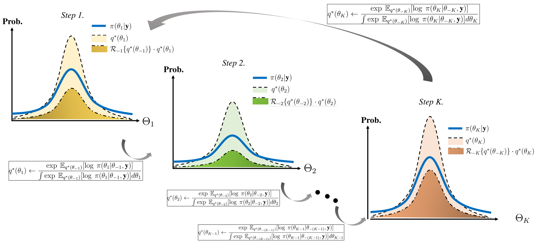
Figure 4: Pictorial illustration of CAVI algorithm (Algorithm 2). At the ii-th step within a cycle (i=1,⋯,Ki=1,\cdots,K), the panel shows that the ii-th variational factor q∗​(θi)q^{*}(\theta_{i}) (14) is pressed from above by the squashing constant ℛ−i​{q∗​(θ−i)}∈(0,1]\mathcal{R}_{-i}\{q^{*}(\theta_{-i})\}\in(0,1] so that it holds ℛ−i​{q∗​(θ−i)}⋅q∗​(θi)≤π⁡(θi|y)\mathcal{R}_{-i}\{q^{*}(\theta_{-i})\}\cdot q^{*}(\theta_{i})\leq\pi(\theta_{i}|\textbf{y}) on Θi\Theta_{i}. The distributional gap between q∗​(θi)q^{*}(\theta_{i}) and π⁡(θi|y)\pi(\theta_{i}|\textbf{y}) is explained by the inequality (30).

See Figure 4 for a pictorial illustration of the Corollary 6.1. Corollary 6.1 (a) implies that, at the ii-th step of the CAVI algorithm (Algorithm 2) (i=1,⋯,Ki=1,\cdots,K), the ii-th variational factor q∗​(θi)∈𝒬θi|ymq^{*}(\theta_{i})\in\mathcal{Q}_{\theta_{i}|\textbf{y}}^{m} (14) and the ii-th marginal target density π⁡(θi|y)∈𝒬θi|ym\pi(\theta_{i}|\textbf{y})\in\mathcal{Q}_{\theta_{i}|\textbf{y}}^{m} are related by the inequality (29) with the squashing constant ℛ−i​{q∗​(θ−i)}\mathcal{R}_{-i}\{q^{*}(\theta_{-i})\}, the functional value of ℛ−i​{⋅}\mathcal{R}_{-i}\{\cdot\} evaluated at q∗​(θ−i)=∏j=1,j≠iKq∗​(θj)∈𝒬θ−i|yM​Fq^{*}(\theta_{-i})=\prod_{j=1,j\neq i}^{K}q^{*}(\theta_{j})\in\mathcal{Q}_{\theta_{-i}|\textbf{y}}^{MF}. More colloquially, the variational factor q∗​(θi)q^{*}(\theta_{i}) (14) can be pressed from above by the squashing constant ℛ−i​{q∗​(θ−i)}\mathcal{R}_{-i}\{q^{*}(\theta_{-i})\}, and kept below than π⁡(θi|y)\pi(\theta_{i}|\textbf{y}). Corollary 6.1 (b) suggests that the denominator in the CAVI formula (14) plays an important role by participating as a lower bound of the distance KL(q∗(θi)||π(θi|y))\text{KL}(q^{*}(\theta_{i})||\pi(\theta_{i}|\textbf{y})). Note that the lower bound is algorithm-based, which can be approximated via a Monte Carlo algorithm.

7 Summary

In this paper, we aimed to provide some pedagogical insights about the Gibbs sampler (Algorithm 1) and CAVI algorithm (Algorithm 2) by treating fundamental densities used in the schemes as elements of sets of densities. Proofs of theorems contained in the paper are derived from the duality formula (3). The derived theorems helped comprehend some common structures between the Gibbs sampler and CAVI algorithm in a set-theoretical perspective. Among salient findings, one of the key discoveries was that the full conditional posterior distribution can be viewed as the global maximum of a functional induced by the duality formula. This has been extended to a new view on the Gibbs sampler from the perspective of information theory. Additionally, we showed that there is a link between the approximation quality of the CAVI algorithm and the denominator of the variational factor (14).

References

  • Andrieu et al. (2003) Andrieu, C., N. De Freitas, A. Doucet, and M. I. Jordan (2003). An introduction to mcmc for machine learning. Machine learning 50(1-2), 5–43.
  • Baxter (2016) Baxter, R. J. (2016). Exactly solved models in statistical mechanics. Elsevier.
  • Beal (2003) Beal, M. J. (2003). Variational algorithms for approximate Bayesian inference. Ph. D. thesis, UCL (University College London).
  • Beichl and Sullivan (2000) Beichl, I. and F. Sullivan (2000). The metropolis algorithm. Computing in Science & Engineering 2(1), 65–69.
  • Bickel et al. (2013) Bickel, P., D. Choi, X. Chang, H. Zhang, et al. (2013). Asymptotic normality of maximum likelihood and its variational approximation for stochastic blockmodels. Annals of Statistics 41(4), 1922–1943.
  • Billingsley (2008) Billingsley, P. (2008). Probability and measure. John Wiley & Sons.
  • Bishop (2006) Bishop, C. M. (2006). Pattern recognition and machine learning. springer.
  • Blei et al. (2006) Blei, D. M., M. I. Jordan, et al. (2006). Variational inference for dirichlet process mixtures. Bayesian analysis 1(1), 121–143.
  • Blei et al. (2017) Blei, D. M., A. Kucukelbir, and J. D. McAuliffe (2017). Variational inference: A review for statisticians. Journal of the American statistical Association 112(518), 859–877.
  • Casella and George (1992) Casella, G. and E. I. George (1992). Explaining the gibbs sampler. The American Statistician 46(3), 167–174.
  • Celisse et al. (2012) Celisse, A., J.-J. Daudin, L. Pierre, et al. (2012). Consistency of maximum-likelihood and variational estimators in the stochastic block model. Electronic Journal of Statistics 6, 1847–1899.
  • Chandler (1987) Chandler, D. (1987). Introduction to modern statistical. Mechanics. Oxford University Press, Oxford, UK.
  • Chib and Greenberg (1995) Chib, S. and E. Greenberg (1995). Understanding the metropolis-hastings algorithm. The american statistician 49(4), 327–335.
  • Cover (1999) Cover, T. M. (1999). Elements of information theory. John Wiley & Sons.
  • Cowles and Carlin (1996) Cowles, M. K. and B. P. Carlin (1996). Markov chain monte carlo convergence diagnostics: a comparative review. Journal of the American Statistical Association 91(434), 883–904.
  • Csiszár et al. (2004) Csiszár, I., P. C. Shields, et al. (2004). Information theory and statistics: A tutorial. Foundations and Trends® in Communications and Information Theory 1(4), 417–528.
  • Dawid (1979) Dawid, A. P. (1979). Conditional independence in statistical theory. Journal of the Royal Statistical Society: Series B (Methodological) 41(1), 1–15.
  • Dwivedi et al. (2018) Dwivedi, R., Y. Chen, M. J. Wainwright, and B. Yu (2018). Log-concave sampling: Metropolis-hastings algorithms are fast! In Conference on Learning Theory, pp. 793–797. PMLR.
  • Gal (2016) Gal, Y. (2016). Uncertainty in deep learning. University of Cambridge 1, 3.
  • Gelfand (2000) Gelfand, A. E. (2000). Gibbs sampling. Journal of the American statistical Association 95(452), 1300–1304.
  • Gelfand and Smith (1990) Gelfand, A. E. and A. F. Smith (1990). Sampling-based approaches to calculating marginal densities. Journal of the American statistical association 85(410), 398–409.
  • Gelman et al. (2013) Gelman, A., J. B. Carlin, H. S. Stern, D. B. Dunson, A. Vehtari, and D. B. Rubin (2013). Bayesian data analysis. CRC press.
  • Geman and Geman (1984) Geman, S. and D. Geman (1984). Stochastic relaxation, gibbs distributions, and the bayesian restoration of images. IEEE Transactions on pattern analysis and machine intelligence (6), 721–741.
  • Jordan et al. (1999) Jordan, M. I., Z. Ghahramani, T. S. Jaakkola, and L. K. Saul (1999). An introduction to variational methods for graphical models. Machine learning 37(2), 183–233.
  • Keener (2010) Keener, R. W. (2010). Theoretical statistics: Topics for a core course. Springer Science & Business Media.
  • Kullback (1997) Kullback, S. (1997). Information theory and statistics. Courier Corporation.
  • Massart (2007) Massart, P. (2007). Concentration inequalities and model selection, Volume 6. Springer.
  • Minka (2013) Minka, T. P. (2013). Expectation propagation for approximate bayesian inference. arXiv preprint arXiv:1301.2294.
  • Murray et al. (2010) Murray, I., R. Adams, and D. MacKay (2010). Elliptical slice sampling. In Proceedings of the thirteenth international conference on artificial intelligence and statistics, pp. 541–548. JMLR Workshop and Conference Proceedings.
  • Neal (2003) Neal, R. M. (2003). Slice sampling. Annals of statistics, 705–741.
  • Neal et al. (2011) Neal, R. M. et al. (2011). Mcmc using hamiltonian dynamics. Handbook of markov chain monte carlo 2(11), 2.
  • Ormerod and Wand (2010) Ormerod, J. T. and M. P. Wand (2010). Explaining variational approximations. The American Statistician 64(2), 140–153.
  • Parisi (1988) Parisi, G. (1988). Statistical field theory. Addison-Wesley.
  • Pellet and Elisseeff (2008) Pellet, J.-P. and A. Elisseeff (2008). Using markov blankets for causal structure learning. Journal of Machine Learning Research 9(7).
  • Ranganath et al. (2014) Ranganath, R., S. Gerrish, and D. Blei (2014). Black box variational inference. In Artificial Intelligence and Statistics, pp. 814–822.
  • Resnick (2003) Resnick, S. I. (2003). A probability path. Springer.
  • Roberts and Polson (1994) Roberts, G. O. and N. G. Polson (1994). On the geometric convergence of the gibbs sampler. Journal of the Royal Statistical Society: Series B (Methodological) 56(2), 377–384.
  • Roberts and Smith (1994) Roberts, G. O. and A. F. Smith (1994). Simple conditions for the convergence of the gibbs sampler and metropolis-hastings algorithms. Stochastic processes and their applications 49(2), 207–216.
  • Royden and Fitzpatrick (1988) Royden, H. L. and P. Fitzpatrick (1988). Real analysis, Volume 32. Macmillan New York.
  • Ruder (2016) Ruder, S. (2016). An overview of gradient descent optimization algorithms. arXiv preprint arXiv:1609.04747.
  • Smith and Roberts (1993) Smith, A. F. and G. O. Roberts (1993). Bayesian computation via the gibbs sampler and related markov chain monte carlo methods. Journal of the Royal Statistical Society: Series B (Methodological) 55(1), 3–23.
  • Wang and Blei (2013) Wang, C. and D. M. Blei (2013). Variational inference in nonconjugate models. Journal of Machine Learning Research 14(Apr), 1005–1031.
  • Wang and Blei (2019) Wang, Y. and D. M. Blei (2019). Frequentist consistency of variational bayes. Journal of the American Statistical Association 114(527), 1147–1161.
  • Yao et al. (2018) Yao, Y., A. Vehtari, D. Simpson, and A. Gelman (2018). Yes, but did it work?: Evaluating variational inference. In International Conference on Machine Learning, pp. 5581–5590. PMLR.
  • You et al. (2014) You, C., J. T. Ormerod, and S. Mueller (2014). On variational bayes estimation and variational information criteria for linear regression models. Australian & New Zealand Journal of Statistics 56(1), 73–87.
  • Zhang and Zhou (2020) Zhang, A. Y. and H. H. Zhou (2020). Theoretical and computational guarantees of mean field variational inference for community detection. The Annals of Statistics 48(5), 2575 – 2598.
  • Zhang et al. (2018) Zhang, C., J. Bütepage, H. Kjellström, and S. Mandt (2018). Advances in variational inference. IEEE transactions on pattern analysis and machine intelligence 41(8), 2008–2026.