跳到论文正文
W Papers独立论文阅读器 arXiv:2008.00982 论文正文 计算阅读时间 · 0%
引用这篇论文根据当前论文元数据生成,正式投稿前建议核对。


License: arXiv.org perpetual non-exclusive license
arXiv:2008.00982v2 [quant-ph] 30 Aug 2020

Quantum Zeno dynamics induced atomic entanglement in a hybrid atom-cavity-fiber system

Jiaojiao Chen Affiliation: Hefei Preschool Education College, Hefei 230013, China    Baolong Fang Affiliation: Institute of Advanced Manufacturing Engineering, Hefei University, Anhui 230022, China    Wei Xiong Affiliation: xiongweiphys@hotmail.com Affiliation: Institute of Advanced Manufacturing Engineering, Hefei University, Anhui 230022, China
August 11, 2026
Abstract

Quantum entanglement is important quanum resources in quantum information sicence. Here we propose an approach to preparing atomic quantum entanglement in a hybrid atom-cavity-fiber system. Using quantum Zeno dynamics method, the system evolution states are always split into a series of Zeno invariant subspaces consisting of dark and bright states. By choosing the initial state of the system, the bright states are all neglected and only dark states are kept to build the effective Hamiltonian. By tuning the system parameters, two-atom multiple-dimensional entanglement, two-atom Bell state, and three-atom GHZ state can be realized by one step. Our proposal provides a way to perform quantum information processing with dark states.

pacs
03.67.Mn,03.67.-a,42.50.Pq

I introduction

Quantum entanglement, one of the most intriguing aspects of quantum mechanics, is an essential resource to quantum information science Horodecki2009; Giraldi2001. Therefore, generating a variety of entangled states have been paid much attention in diverse quantum systems Chuang1995; Reina2000; Zheng2000; Unanyan2003. For example, GHZ states, first proposed by Greenberger, Horne, and Zeilinger, provide much stronger refutations of local realism and offer possibilities to test quantum mechanics against local hidden theory without inequality Greenberger90, and it has been demonstrated that violations of local realism by two entangled high-dimensional systems are stronger than that by two-dimensional systems Kaszlikowski00. Thus, much interest has been focused on the generation of high-dimensional entangled states. Among various quantum systems, the emerging hybrid quantum systems, with the goal of harnessing the advantages of different subsystems to better explore new phenomena and potentially bring about novel quantum technologies (see Xiang2013; Kurizki2015 for a review), can have versatile applications in quantum information, especially for the atom-cavity-fiber hybrid systems. Because photons as flying qubits can transfer quantum information fast and atoms as stationary qubits can store quantum information for a long time. In the hybrid atom-cavity-fiber system, highly reliable swap and entangling gates are investigated via resonant interaction Serafini2006. Then a scheme for deterministically realization of a highly reliable quantum swap gate is proposed Yin2007. Later, a resonant interaction scheme for implementing quantum phase gates Chen2015 and a conditional phase gate Zheng2009 via a nonresonant interaction are studied. More recently, a remote swap gate through virtual photon and virtual atomic excitation is achieved Wu2019. Also, proposals of Fredkin Gates and high-dimensional entangled states have been proposed Sun20. Experimentally, dressed states of two separated atoms with the atom-cavity-fiber system have been observed Kato19.

On the other hand, quantum Zeno effect has attracted extensive interest because it hinders the evolution out of the initial state after performing frequent measurements. In 1988, testing the Zeno effect on oscillating (mainly two-level) systems is theoretically proposed Cook1988 and demonstrated experimentally Itano1990 a few years later. In fact, a quantum Zeno evolution does not necessarily freeze the dynamics. By frequently projecting onto a multidimensional subspace, the system will evolve away from its initial state, although it remains in the “Zeno subspace” defined by the measurement Facchi2000; Facchi2001. Moreover, the quantum Zeno effect can be regarded as a continuous measurement Facchi2009 without employing projection operators and nonunitary dynamics. Since then, lots of schemes for preparation of quantum states Luis2001; Wang2008; Li2011; Shen2011 and quantum gates Beige2000; Franson2004; Shao2009; Franson2007 via quantum Zeno dynamics have been proposed.

Based on these advanced works, we propose a scheme based on quantum Zeno dynamics to realize two-atom multiple-dimensional entangled states, two-atom Bell state and three-atom GHZ state in a hybrid atom-cavity-fiber system. In this setup, the six-level atom is trapped in one cavity and the other two atoms with three-level configuration are trapped in the other cavity. Two cavities are connected by a fiber. We find that the six-level atom and one of the three-level atoms can be in non-maximally three-dimensional entangled states depending on the initial state of the six-level atom. When the coupling between the atom and the cavity is comparable to the coupling between the fiber and cavity modes, the maximally three-dimensional quantum entanglement for two separated atoms can be generated. Also, the Bell state for the six-level atom and one of the three-level atoms can be obtained when the coupling between the atom and the cavity is much smaller than the coupling between the fiber and cavity modes, which indicates that not very strong atom-cavity coupling is enough for producing Bell states. Preparing the six-level atoms in a specially initial state, a six-demensional entangled state and GHZ state for three atoms can be achieved. Our setup may provide a way to realize more complicated quantum information processing.

The paper is organized as follows. Section II introduces the physical model of our hybrid system and the method of the quantum Zeno dynamics. In Sec. III, we give a detailed description of producing various entangled states. Finally, we give a short conclusion in Sec. IV.

II Model and quantum Zeno dynamics

II.1 Physical model
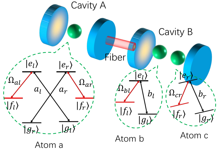
Refer to caption
Figure 1: (Color online) Schematic diagram of the hybrid atom-cavity-fiber system. The atom a with six-level structure is trapped in the cavity A, and atoms b and c with three-level structure are trapped in the cavity B. Two cavities are connected by an optical fiber.

We consider a hybrid quantum system consisting of two optical cavities (labeled as A{A} and B{B}) connected by an optical fiber and three atoms (labeled as atom a,b,c{a},~{b},~{c}) with different level structures (see Fig. 1), where the atom aa is trapped in the cavity AA and the atoms bb and cc are trapped in the cavity BB. The transition between the level |fi⟩j|f_{i}\rangle_{j} and |ei⟩j|e_{i}\rangle_{j} is driven by a driving field with Rabi frequency Ωi​j\Omega_{ij}, where i=l,ri=l,r and j=a,b,cj=a,b,c. The transition between |gi⟩a|g_{i}\rangle_{a} and |ei⟩a|e_{i}\rangle_{a} of the atom aa is coupled to the ii mode of the cavity AA, and the transition between |gi⟩b⁡(c)|g_{i}\rangle_{b(c)} and |ei⟩b⁡(c)|e_{i}\rangle_{b(c)} of the atom b⁡(c)b~(c) is coupled to the ii mode of the cavity BB. In the short fiber regime, i.e., 2​L​ν¯/2​π​c≤12L\bar{\nu}/2\pi c\leq 1, the ii mode of the fiber can be only coupled to the ii-mode of the cavities AA and BB. Here, LL is the length of the optical fiber, ν¯\bar{\nu} is the decay rate of the cavity fields flowing into a continuum of the fiber modes, and cc is the speed of light in vacuum. In the interaction representation, the total Hamitlonian of the hybrid quantum system within the rotating wave approximation can be governed by (setting ℏ=1\hbar=1)

Ht​o​t=Ha​c+Hc​f+Hd,\displaystyle H_{tot}=H_{ac}+H_{cf}+H_{d}, (1)

where

Ha​c=\displaystyle H_{ac}= ga​l​|el⟩a​a​⟨gl|cA​l+ga​r|er⟩a​a​⟨gr|​cA​r\displaystyle g_{al}|e_{l}\rangle_{aa}\langle g_{l}|c_{Al}+g_{ar}|e_{r}\rangle_{aa}\langle g_{r}|c_{Ar}
+gb​l​|el⟩b​b​⟨gl|cB​l+gc​r|er⟩c​c​⟨gr|​cB​r+H.c.,\displaystyle+g_{bl}|e_{l}\rangle_{bb}\langle g_{l}|c_{Bl}+g_{cr}|e_{r}\rangle_{cc}\langle g_{r}|c_{Br}+{\rm H.c.},
Hc​f=\displaystyle H_{cf}= λl​dl†​(cA​l+cB​l)+λr​dr†​(cA​r+cB​r)+H.c.,\displaystyle\lambda_{l}d_{l}^{\dagger}(c_{Al}+c_{Bl})+\lambda_{r}d_{r}^{\dagger}(c_{Ar}+c_{Br})+{\rm H.c.},
Hd=\displaystyle H_{d}= Ωa​l​|el⟩a​a​⟨fl|+Ωa​r|er⟩a​a​⟨fr|+Ωb​l|el⟩b​b​⟨fl|\displaystyle\Omega_{al}|e_{l}\rangle_{aa}\langle f_{l}|+\Omega_{ar}|e_{r}\rangle_{aa}\langle f_{r}|+\Omega_{bl}|e_{l}\rangle_{bb}\langle f_{l}|
+Ωc​r​|er⟩c​c​⟨fr|+H.c.,\displaystyle+\Omega_{cr}|e_{r}\rangle_{cc}\langle f_{r}|+{\rm H.c.}, (2)

where the first term Ha​cH_{ac} in Eq. (1) describes the interaction between the atoms and cavities with coupling strengths ga​l,gb​lg_{al},~g_{bl} and gc​rg_{cr}. The second term Hc​fH_{cf} in Eq. (1) describes the coupling between the ii mode of the optical fiber and the ii mode of the cavities AA andBB with coupling strength λi\lambda_{i}. The last term HdH_{d} in Eq. (1) describes the interaction between the atom and the driving fields. The operators cA​ic_{Ai} and cB​ic_{Bi} are the annihilation operators of the ii mode of the cavities AA and BB, and H.c.{\rm H.c.} in Eq. (2) denotes the hermitian conjugate.

From Eq. (1), atom aa initially prepared in the state |fi⟩a|f_{i}\rangle_{a} will be excited to the state |ei⟩a|e_{i}\rangle_{a}, then a photon arising from ii mode is produced due to the coupling between the ii mode of the cavity AA and the transition |ei⟩a↔|gi⟩a|e_{i}\rangle_{a}\leftrightarrow|g_{i}\rangle_{a} of the atom aa. The generated photon can flow into the cavity BB via the interaction between the fiber and the cavities AA or BB. Once the photon generated from the cavity AA enters the cavity BB, it will excite the state |gl⟩|g_{l}\rangle to |el⟩|e_{l}\rangle of the atom bb or the state |gr⟩|g_{r}\rangle to |er⟩|e_{r}\rangle of the atom cc, and vice versa.

II.2 Quantum Zeno dynamics

Now we briefly give a review about the quantum Zeno dynamcis induced by continuous coupling. We suppose a dynamical evolution process is governed by

HK=HS+K​HC,\displaystyle H_{K}=H_{S}+KH_{C}, (3)

where HSH_{S} is the Hamiltonian of the subsystem to be investigated and HCH_{C} is an additional interaction Hamiltonian which performs the measurement, KK is the coupling strength. For a large KK, i.e., K→∞K\rightarrow\infty, the subsystem of interest is dominated by the following evolution operator

𝒱⁡(t)=limK→∞exp⁡(i​K​HC​t)​V​(t).\displaystyle\mathcal{V}(t)=\lim_{K\rightarrow\infty}\exp(iKH_{C}t)V(t). (4)

Equivalently,

𝒱⁡(t)=exp⁡(−i​HZ​t)\displaystyle\mathcal{V}(t)=\exp(-iH_{Z}t) (5)

with

HZ=∑nPn​HS​Pn\displaystyle H_{Z}=\sum_{n}P_{n}H_{S}P_{n} (6)

being the Zeno Hamiltonian, in which PnP_{n} is the eigenprojection of the HCH_{C} belonging to the corresponding eigenvalue EnE_{n},

HC=∑nEn​Pn.\displaystyle H_{C}=\sum_{n}E_{n}P_{n}. (7)

Thus the whole system is governed by the limiting evolution operator

VK​(t)=exp⁡(−i​Heff​t)\displaystyle V_{K}(t)=\exp(-iH_{\rm eff}t) (8)

with

Heff=∑nK​En​Pn​t+Pn​HS​Pn.\displaystyle H_{\rm eff}=\sum_{n}KE_{n}P_{n}t+P_{n}H_{S}P_{n}. (9)

This equation is the important result governing our following works.

III The dynamics of the hybrid quantum system

To begin our task, we for convenience assume ga​l=ga​r=gb​l=gc​r=gg_{al}=g_{ar}=g_{bl}=g_{cr}=g, Ωa​l=Ωa​r=Ω1\Omega_{al}=\Omega_{ar}=\Omega_{1}, Ωb​l=Ω2\Omega_{bl}=\Omega_{2}, Ωc​r=Ω3\Omega_{cr}=\Omega_{3}, λl=λr=λ\lambda_{l}=\lambda_{r}=\lambda. Also, the single-photon excitation approximation is assumed in the process of the dynamics evolution.

III.1 Initial state |fl⟩a​|gl⟩b​|gr⟩c​|0l​0r⟩A​|0l​0r⟩B​|0l​0r⟩F|f_{l}\rangle_{a}|g_{l}\rangle_{b}|g_{r}\rangle_{c}|0_{l}0_{r}\rangle_{A}|0_{l}0_{r}\rangle_{B}|0_{l}0_{r}\rangle_{F}

Based on above analysis, we initially prepare the hybrid system in the state

|ψ0⟩=|fl⟩a​|gl⟩b​|gr⟩c​|0l​0r⟩A​|0l​0r⟩B​|0l​0r⟩F,\displaystyle|\psi_{0}\rangle=|f_{l}\rangle_{a}|g_{l}\rangle_{b}|g_{r}\rangle_{c}|0_{l}0_{r}\rangle_{A}|0_{l}0_{r}\rangle_{B}|0_{l}0_{r}\rangle_{F}, (10)

which indicates that the atom aa is initially prepared in the state |fl⟩a|f_{l}\rangle_{a}, both the atoms bb and cc are respectively in the states |gl⟩b|g_{l}\rangle_{b} and |gr⟩c|g_{r}\rangle_{c}, the cavities AA, BB and the fiber are all in their vacuum states. Under the interaction of the Hamiltonian (1), seven states are generated constructing a evolution subspace spanned by

U1={|ϕ0⟩,|ϕ1⟩,|ϕ2⟩,|ϕ3⟩,|ϕ4⟩,|ϕ5⟩,|ϕ6⟩},\displaystyle U_{1}=\bigg\{|\phi_{0}\rangle,|\phi_{1}\rangle,|\phi_{2}\rangle,|\phi_{3}\rangle,|\phi_{4}\rangle,|\phi_{5}\rangle,|\phi_{6}\rangle\bigg\}, (11)

with

|ϕ0⟩=\displaystyle|\phi_{0}\rangle= |ψ0⟩,\displaystyle|\psi_{0}\rangle,
|ϕ1⟩=\displaystyle|\phi_{1}\rangle= |el⟩a​|gl⟩b​|gr⟩c​|0l​0r⟩A​|0l​0r⟩B​|0l​0r⟩F,\displaystyle|e_{l}\rangle_{a}|g_{l}\rangle_{b}|g_{r}\rangle_{c}|0_{l}0_{r}\rangle_{A}|0_{l}0_{r}\rangle_{B}|0_{l}0_{r}\rangle_{F},
|ϕ2⟩=\displaystyle|\phi_{2}\rangle= |gl⟩a​|gl⟩b​|gr⟩c​|1l​0r⟩A​|0l​0r⟩B​|0l​0r⟩F,\displaystyle|g_{l}\rangle_{a}|g_{l}\rangle_{b}|g_{r}\rangle_{c}|1_{l}0_{r}\rangle_{A}|0_{l}0_{r}\rangle_{B}|0_{l}0_{r}\rangle_{F},
|ϕ3⟩=\displaystyle|\phi_{3}\rangle= |gl⟩a​|gl⟩b​|gr⟩c​|0l​0r⟩A​|0l​0r⟩B​|1l​0r⟩F,\displaystyle|g_{l}\rangle_{a}|g_{l}\rangle_{b}|g_{r}\rangle_{c}|0_{l}0_{r}\rangle_{A}|0_{l}0_{r}\rangle_{B}|1_{l}0_{r}\rangle_{F},
|ϕ4⟩=\displaystyle|\phi_{4}\rangle= |gl⟩a​|gl⟩b​|gr⟩c​|0l​0r⟩A​|1l​0r⟩B​|0l​0r⟩F,\displaystyle|g_{l}\rangle_{a}|g_{l}\rangle_{b}|g_{r}\rangle_{c}|0_{l}0_{r}\rangle_{A}|1_{l}0_{r}\rangle_{B}|0_{l}0_{r}\rangle_{F},
|ϕ5⟩=\displaystyle|\phi_{5}\rangle= |gl⟩a​|el⟩b​|gr⟩c​|0l​0r⟩A​|0l​0r⟩B​|0l​0r⟩F,\displaystyle|g_{l}\rangle_{a}|e_{l}\rangle_{b}|g_{r}\rangle_{c}|0_{l}0_{r}\rangle_{A}|0_{l}0_{r}\rangle_{B}|0_{l}0_{r}\rangle_{F},
|ϕ6⟩=\displaystyle|\phi_{6}\rangle= |gl⟩a​|fl⟩b​|gr⟩c​|0l​0r⟩A​|0l​0r⟩B​|0l​0r⟩F.\displaystyle|g_{l}\rangle_{a}|f_{l}\rangle_{b}|g_{r}\rangle_{c}|0_{l}0_{r}\rangle_{A}|0_{l}0_{r}\rangle_{B}|0_{l}0_{r}\rangle_{F}.

Using these basis, the interaction Hamiltonian (1) can be rewritten as

H1=(0Ω100000Ω10g00000g0λ00000λ0λ00000λ0g00000g0Ω200000Ω20).\displaystyle H_{1}=\begin{pmatrix}0&\Omega_{1}&0&0&0&0&0\\ \Omega_{1}&0&g&0&0&0&0\\ 0&g&0&\lambda&0&0&0\\ 0&0&\lambda&0&\lambda&0&0\\ 0&0&0&\lambda&0&g&0\\ 0&0&0&0&g&0&\Omega_{2}\\ 0&0&0&0&0&\Omega_{2}&0\\ \end{pmatrix}. (12)

The eigenvectors of Hamiltonian (12) within the asuumption of {Ω1,Ω2}≪{g,λ}\{\Omega_{1},\Omega_{2}\}\ll\{g,\lambda\}, consisting of dark states (|D0⟩,D1⟩,|D2⟩|D_{0}\rangle,~D_{1}\rangle,~|D_{2}\rangle) with zero eigenvalues and bright states (|B0⟩,B1⟩,|B2⟩,|B3⟩|B_{0}\rangle,~B_{1}\rangle,~|B_{2}\rangle,~|B_{3}\rangle) with non-zero values, are

|D0⟩=\displaystyle|D_{0}\rangle= |ϕ0⟩,|D1⟩=|ϕ6⟩,\displaystyle|\phi_{0}\rangle,~~|D_{1}\rangle=|\phi_{6}\rangle,
|D2⟩=\displaystyle|D_{2}\rangle= λg​χ​(|ϕ1⟩−gλ​|ϕ3⟩+|ϕ5⟩),\displaystyle\frac{\lambda}{g\chi}(|\phi_{1}\rangle-\frac{g}{\lambda}|\phi_{3}\rangle+|\phi_{5}\rangle),
|B0⟩=\displaystyle|B_{0}\rangle= 12​(−|ϕ1⟩−|ϕ2⟩+|ϕ4⟩+|ϕ5⟩),\displaystyle\frac{1}{2}(-|\phi_{1}\rangle-|\phi_{2}\rangle+|\phi_{4}\rangle+|\phi_{5}\rangle),
|B1⟩=\displaystyle|B_{1}\rangle= 12​(−|ϕ1⟩+|ϕ2⟩−|ϕ4⟩+|ϕ5⟩),\displaystyle\frac{1}{2}(-|\phi_{1}\rangle+|\phi_{2}\rangle-|\phi_{4}\rangle+|\phi_{5}\rangle),
|B2⟩=\displaystyle|B_{2}\rangle= 2​χ​(|ϕ1⟩+χ⁡|ϕ2⟩+λg​|ϕ3⟩−χ⁡|ϕ4⟩+|ϕ5⟩),\displaystyle 2\chi(|\phi_{1}\rangle+\chi|\phi_{2}\rangle+\frac{\lambda}{g}|\phi_{3}\rangle-\chi|\phi_{4}\rangle+|\phi_{5}\rangle),
|B3⟩=\displaystyle|B_{3}\rangle= 2​χ​(|ϕ1⟩−χ⁡|ϕ2⟩+λg​|ϕ3⟩−χ⁡|ϕ4⟩+|ϕ5⟩),\displaystyle 2\chi(|\phi_{1}\rangle-\chi|\phi_{2}\rangle+\frac{\lambda}{g}|\phi_{3}\rangle-\chi|\phi_{4}\rangle+|\phi_{5}\rangle), (13)

where χ=(1+2​λ2/g2)12\chi=(1+2\lambda^{2}/g^{2})^{\frac{1}{2}} and the correspinding eigenvalues are E0=0,E1=0,E2=0,E3=g,E4=−g,E5=g​χ,E6=−g​χE_{0}=0,~E_{1}=0,~E_{2}=0,~E_{3}=g,~E_{4}=-g,~E_{5}=g\chi,~E_{6}=-g\chi. Note that the whole Hilbert subspace for Hamiltonian (12) under {Ω1,Ω2}≪{g,λ}\{\Omega_{1},\Omega_{2}\}\ll\{g,\lambda\} can be divided into five invariant subspaces as following,

Γp0=\displaystyle\Gamma_{p_{0}}= {|D0⟩,|D1⟩,|D2⟩},Γp1={|B0⟩}\displaystyle\{|D_{0}\rangle,|D_{1}\rangle,|D_{2}\rangle\},~\Gamma_{p_{1}}=\{|B_{0}\rangle\}
Γp2=\displaystyle\Gamma_{p_{2}}= {|B1⟩},Γp3={|B2⟩},Γp4={|B3⟩}.\displaystyle\{|B_{1}\rangle\},~\Gamma_{p_{3}}=\{|B_{2}\rangle\},~\Gamma_{p_{4}}=\{|B_{3}\rangle\}. (14)

Here pj=|α⟩​⟨α|p_{j}=|\alpha\rangle\langle\alpha| with j=0,1,2,3,4j=0,1,2,3,4 is the projector and α∈{Γp0,Γp1,Γp2,Γp3,Γp4}\alpha\in\{\Gamma_{p_{0}},\Gamma_{p_{1}},\Gamma_{p_{2}},\Gamma_{p_{3}},\Gamma_{p_{4}}\}. According to quantum Zeno dynamics method, the Hamiltonian in Eq. (12) reduces to

ℋ1=\displaystyle\mathcal{H}_{1}= ∑j=0Ej​pj+pj​Hd​pj\displaystyle\sum_{j=0}E_{j}p_{j}+p_{j}H_{d}p_{j}
=\displaystyle= g⁡[|B0⟩​⟨B0|−|B1⟩​⟨B1|+χ⁡(|B2⟩​⟨B2|−|B3⟩​⟨B3|)]\displaystyle g\big[|B_{0}\rangle\langle B_{0}|-|B_{1}\rangle\langle B_{1}|+\chi(|B_{2}\rangle\langle B_{2}|-|B_{3}\rangle\langle B_{3}|)\big]
+λg​χ(Ω1|D0⟩⟨D2|+Ω2|D1⟩⟨D2|+H.c.).\displaystyle+\frac{\lambda}{g\chi}(\Omega_{1}|D_{0}\rangle\langle D_{2}|+\Omega_{2}|D_{1}\rangle\langle D_{2}|+{\rm H.c.}). (15)

Since the system is initially prepared in the state |D0⟩|D_{0}\rangle, the system will always evolve in the Zeno subspace spanned by{|D0⟩,|D2⟩,|B2⟩}\{|D_{0}\rangle,|D_{2}\rangle,|B_{2}\rangle\}. The corresponding dynamics can be governed by the effective Hamiltonian

Heff=λg​χ(Ω1|D0⟩⟨D2|+Ω2|D1⟩⟨D2|+H.c.),\displaystyle H_{\rm eff}=\frac{\lambda}{g\chi}(\Omega_{1}|D_{0}\rangle\langle D_{2}|+\Omega_{2}|D_{1}\rangle\langle D_{2}|+{\rm H.c.}), (16)

and at time τ\tau, the system state is

|ψτ⟩=e−i​Heff​τ​|ψ0⟩=A1​|D0⟩+A2​|D2⟩+A3​|D1⟩,\displaystyle|\psi_{\tau}\rangle=e^{-iH_{\rm eff}\tau}|\psi_{0}\rangle=A_{1}|D_{0}\rangle+A_{2}|D_{2}\rangle+A_{3}|D_{1}\rangle, (17)

where

A1=\displaystyle A_{1}= sin2⁡θ+cos2⁡θ​cos⁡(Ω​λ​τ/g​χ),\displaystyle\sin^{2}\theta+\cos^{2}\theta\cos(\Omega\lambda\tau/g\chi),
A2=\displaystyle A_{2}= −i​cos⁡θ​sin⁡(Ω​λ​τ/g​χ)\displaystyle-i\cos\theta\sin(\Omega\lambda\tau/g\chi)
A3=\displaystyle A_{3}= 12​sin⁡(2​θ)​[cos⁡(Ω​λ​τ/g​χ)−1]\displaystyle\frac{1}{2}\sin(2\theta)\big[\cos(\Omega\lambda\tau/g\chi)-1\big] (18)

with Ω12+Ω22=Ω2\Omega_{1}^{2}+\Omega_{2}^{2}=\Omega^{2} and tan⁡θ=Ω2/Ω1\tan\theta=\Omega_{2}/\Omega_{1}. By controlling the system parameters {Ω1,Ω2,λ,g,τ}\{\Omega_{1},\Omega_{2},\lambda,g,\tau\}, different quantum information task can be achieved. For example, when Ω2≪Ω1\Omega_{2}\ll\Omega_{1}, sin⁡θ→0\sin\theta\rightarrow 0 and cos⁡θ→1\cos\theta\rightarrow 1. Thus, A1→cos⁡(Ω​λ​τ/g​χ)A_{1}\rightarrow\cos(\Omega\lambda\tau/g\chi), A2→−i​sin⁡(Ω​λ​τ/g​χ)A_{2}\rightarrow-i\sin(\Omega\lambda\tau/g\chi) and A3→0A_{3}\rightarrow 0. Then we choose Ω​λ​τ/g​χ=(2​k−1)​π/2\Omega\lambda\tau/g\chi=(2k-1)\pi/2 with k=1,2,3,…k=1,2,3,..., leading to cos⁡(Ω​λ​τ/g​χ)=0\cos(\Omega\lambda\tau/g\chi)=0 and cos⁡(Ω​λ​τ/g​χ)=1\cos(\Omega\lambda\tau/g\chi)=1. This condition can be achieved by tuning the parameters {Ω1,Ω2,λ,g,τ}\{\Omega_{1},\Omega_{2},\lambda,g,\tau\}, which greatly reduces the difficulties experimentally. With this condition, Eq. (17) becomes

|ψτ⟩ST=−i⁡|D2⟩,\displaystyle|\psi_{\tau}\rangle_{\rm ST}=-i|D_{2}\rangle, (19)

which indicates quantum state transition between two degenerate states is allowed and the state |D1⟩|D_{1}\rangle is safely neglected. Note that when the photons in the ll mode of the optical fiber experience a Hadamard gate, i.e., |0⟩→12​(|0⟩+|1⟩)|0\rangle\rightarrow\frac{1}{\sqrt{2}}(|0\rangle+|1\rangle) and |1⟩→12​(|0⟩−|1⟩)|1\rangle\rightarrow\frac{1}{\sqrt{2}}(|0\rangle-|1\rangle), and then trace the degrees of the freedom of the atom bb and the photons in the cavity and fiber modes out, the quantum state in Eq. (19) further reduces to

|ψτ⟩TD=13​(|el⟩​|gl⟩−|gl⟩​|gl⟩+|gl⟩​|el⟩)a​b\displaystyle|\psi_{\tau}\rangle_{\rm TD}=\frac{1}{\sqrt{3}}(|e_{l}\rangle|g_{l}\rangle-|g_{l}\rangle|g_{l}\rangle+|g_{l}\rangle|e_{l}\rangle)_{ab} (20)

by setting g=λg=\lambda, which is a three-dimensional quantum entanglement between atoms aa and bb. However, when g≪λg\ll\lambda, Eq. (19) describes a Bell state between atoms aa and bb, i.e.,

|ψτ⟩Bell=12​(|el⟩​|gl⟩+|gl⟩​|el⟩)a​b.\displaystyle|\psi_{\tau}\rangle_{\rm Bell}=\frac{1}{\sqrt{2}}(|e_{l}\rangle|g_{l}\rangle+|g_{l}\rangle|e_{l}\rangle)_{ab}. (21)

On the other hand, Eq. (17) can be rewritten as

|ψτ⟩SW=|D1⟩\displaystyle|\psi_{\tau}\rangle_{\rm SW}=|D_{1}\rangle (22)

by setting Ω1=Ω2=Ω/2\Omega_{1}=\Omega_{2}=\Omega/\sqrt{2} and Ω​λ​τ/g​χ=k​π\Omega\lambda\tau/g\chi=k\pi with k=1,2,3,…k=1,2,3,.... This implies that state swapping (|fl⟩a​|gl⟩b↔|gl⟩a​|fl⟩b|f_{l}\rangle_{a}|g_{l}\rangle_{b}\leftrightarrow|g_{l}\rangle_{a}|f_{l}\rangle_{b}) between atoms aa and bb is achieved.

III.2 Initial state |fr⟩a​|gl⟩b​|gr⟩c​|0l​0r⟩A​|0l​0r⟩B​|0l​0r⟩F|f_{r}\rangle_{a}|g_{l}\rangle_{b}|g_{r}\rangle_{c}|0_{l}0_{r}\rangle_{A}|0_{l}0_{r}\rangle_{B}|0_{l}0_{r}\rangle_{F}

Below we assume that the initial state of the atom-cavity-fiber hybrid system is

|ψ0′⟩=|fr⟩a​|gl⟩b​|gr⟩c​|0l​0r⟩A​|0l​0r⟩B​|0l​0r⟩F,\displaystyle|\psi_{0}^{\prime}\rangle=|f_{r}\rangle_{a}|g_{l}\rangle_{b}|g_{r}\rangle_{c}|0_{l}0_{r}\rangle_{A}|0_{l}0_{r}\rangle_{B}|0_{l}0_{r}\rangle_{F}, (23)

which indicates that the atom aa is initially prepared in the state |fr⟩a|f_{r}\rangle_{a}, both the atoms bb and cc are respectively in the states |gl⟩b|g_{l}\rangle_{b} and |gr⟩c|g_{r}\rangle_{c}, the cavities AA, BB and the fiber are all in their vacuum states. Under the interaction of the Hamiltonian (1), seven states are generated constructing a evolution subspace spanned by

U1′={|ϕ0′⟩,|ϕ1′⟩,|ϕ2′⟩,|ϕ3′⟩,|ϕ4′⟩,|ϕ5′⟩,|ϕ6′⟩},\displaystyle U_{1}^{\prime}=\bigg\{|\phi_{0}^{\prime}\rangle,|\phi_{1}^{\prime}\rangle,|\phi_{2}^{\prime}\rangle,|\phi_{3}^{\prime}\rangle,|\phi_{4}^{\prime}\rangle,|\phi_{5}^{\prime}\rangle,|\phi_{6}^{\prime}\rangle\bigg\}, (24)

with

|ϕ0′⟩=\displaystyle|\phi_{0}^{\prime}\rangle= |ψ0′⟩,\displaystyle|\psi_{0}^{\prime}\rangle,
|ϕ1′⟩=\displaystyle|\phi_{1}^{\prime}\rangle= |er⟩a​|gl⟩b​|gr⟩c​|0l​0r⟩A​|0l​0r⟩B​|0l​0r⟩F,\displaystyle|e_{r}\rangle_{a}|g_{l}\rangle_{b}|g_{r}\rangle_{c}|0_{l}0_{r}\rangle_{A}|0_{l}0_{r}\rangle_{B}|0_{l}0_{r}\rangle_{F},
|ϕ2′⟩=\displaystyle|\phi_{2}^{\prime}\rangle= |gr⟩a​|gl⟩b​|gr⟩c​|1l​0r⟩A​|0l​0r⟩B​|0l​0r⟩F,\displaystyle|g_{r}\rangle_{a}|g_{l}\rangle_{b}|g_{r}\rangle_{c}|1_{l}0_{r}\rangle_{A}|0_{l}0_{r}\rangle_{B}|0_{l}0_{r}\rangle_{F},
|ϕ3′⟩=\displaystyle|\phi_{3}^{\prime}\rangle= |gr⟩a​|gl⟩b​|gr⟩c​|0l​0r⟩A​|0l​0r⟩B​|0l​1r⟩F,\displaystyle|g_{r}\rangle_{a}|g_{l}\rangle_{b}|g_{r}\rangle_{c}|0_{l}0_{r}\rangle_{A}|0_{l}0_{r}\rangle_{B}|0_{l}1_{r}\rangle_{F},
|ϕ4′⟩=\displaystyle|\phi_{4}^{\prime}\rangle= |gr⟩a​|gl⟩b​|gr⟩c​|0l​0r⟩A​|0l​1r⟩B​|0l​0r⟩F,\displaystyle|g_{r}\rangle_{a}|g_{l}\rangle_{b}|g_{r}\rangle_{c}|0_{l}0_{r}\rangle_{A}|0_{l}1_{r}\rangle_{B}|0_{l}0_{r}\rangle_{F},
|ϕ5′⟩=\displaystyle|\phi_{5}^{\prime}\rangle= |gr⟩a​|gl⟩b​|er⟩c​|0l​0r⟩A​|0l​0r⟩B​|0l​0r⟩F,\displaystyle|g_{r}\rangle_{a}|g_{l}\rangle_{b}|e_{r}\rangle_{c}|0_{l}0_{r}\rangle_{A}|0_{l}0_{r}\rangle_{B}|0_{l}0_{r}\rangle_{F},
|ϕ6′⟩=\displaystyle|\phi_{6}^{\prime}\rangle= |gr⟩a​|gl⟩b​|fr⟩c​|0l​0r⟩A​|0l​0r⟩B​|0l​0r⟩F.\displaystyle|g_{r}\rangle_{a}|g_{l}\rangle_{b}|f_{r}\rangle_{c}|0_{l}0_{r}\rangle_{A}|0_{l}0_{r}\rangle_{B}|0_{l}0_{r}\rangle_{F}.

Using these basis, the interaction Hamiltonian (1) can be rewritten as

H1′=(0Ω100000Ω10g00000g0λ00000λ0λ00000λ0g00000g0Ω300000Ω30).\displaystyle H_{1}^{\prime}=\begin{pmatrix}0&\Omega_{1}&0&0&0&0&0\\ \Omega_{1}&0&g&0&0&0&0\\ 0&g&0&\lambda&0&0&0\\ 0&0&\lambda&0&\lambda&0&0\\ 0&0&0&\lambda&0&g&0\\ 0&0&0&0&g&0&\Omega_{3}\\ 0&0&0&0&0&\Omega_{3}&0\\ \end{pmatrix}. (25)

The eigenvectors of Hamiltonian (25) within the asuumption of {Ω1,Ω3}≪{g,λ}\{\Omega_{1},\Omega_{3}\}\ll\{g,\lambda\}, consisting of dark states (|D0′⟩,D1′⟩,|D2′⟩|D_{0}^{\prime}\rangle,~D_{1}^{\prime}\rangle,~|D_{2}^{\prime}\rangle) with zero eigenvalues and bright states (|B0′⟩,B1′⟩,|B2′⟩,|B3′⟩|B_{0}^{\prime}\rangle,~B_{1}^{\prime}\rangle,~|B_{2}^{\prime}\rangle,~|B_{3}^{\prime}\rangle) with non-zero values, are

|D0′⟩=\displaystyle|D_{0}^{\prime}\rangle= |ϕ0′⟩,|D1′⟩=|ϕ6′⟩,\displaystyle|\phi_{0}^{\prime}\rangle,~~|D_{1}^{\prime}\rangle=|\phi_{6}^{\prime}\rangle,
|D2′⟩=\displaystyle|D_{2}^{\prime}\rangle= λg​χ​(|ϕ1′⟩−gλ​|ϕ3′⟩+|ϕ5′⟩),\displaystyle\frac{\lambda}{g\chi}(|\phi_{1}^{\prime}\rangle-\frac{g}{\lambda}|\phi_{3}^{\prime}\rangle+|\phi_{5}^{\prime}\rangle),
|B0′⟩=\displaystyle|B_{0}^{\prime}\rangle= 12​(−|ϕ1′⟩−|ϕ2′⟩+|ϕ4′⟩+|ϕ5′⟩),\displaystyle\frac{1}{2}(-|\phi_{1}^{\prime}\rangle-|\phi_{2}^{\prime}\rangle+|\phi_{4}^{\prime}\rangle+|\phi_{5}^{\prime}\rangle),
|B1′⟩=\displaystyle|B_{1}^{\prime}\rangle= 12​(−|ϕ1′⟩+|ϕ2′⟩−|ϕ4′⟩+|ϕ5′⟩),\displaystyle\frac{1}{2}(-|\phi_{1}^{\prime}\rangle+|\phi_{2}^{\prime}\rangle-|\phi_{4}^{\prime}\rangle+|\phi_{5}^{\prime}\rangle),
|B2′⟩=\displaystyle|B_{2}^{\prime}\rangle= 2​χ​(|ϕ1′⟩+χ⁡|ϕ2′⟩+λg​|ϕ3′⟩−χ⁡|ϕ4′⟩+|ϕ5′⟩),\displaystyle 2\chi(|\phi_{1}^{\prime}\rangle+\chi|\phi_{2}^{\prime}\rangle+\frac{\lambda}{g}|\phi_{3}^{\prime}\rangle-\chi|\phi_{4}^{\prime}\rangle+|\phi_{5}^{\prime}\rangle),
|B3′⟩=\displaystyle|B_{3}^{\prime}\rangle= 2​χ​(|ϕ1′⟩−χ⁡|ϕ2′⟩+λg​|ϕ3′⟩−χ⁡|ϕ4′⟩+|ϕ5′⟩),\displaystyle 2\chi(|\phi_{1}^{\prime}\rangle-\chi|\phi_{2}^{\prime}\rangle+\frac{\lambda}{g}|\phi_{3}^{\prime}\rangle-\chi|\phi_{4}^{\prime}\rangle+|\phi_{5}^{\prime}\rangle), (26)

where χ=(1+2​λ2/g2)12\chi=(1+2\lambda^{2}/g^{2})^{\frac{1}{2}} and the correspinding eigenvalues are E0′=0,E1′=0,E2′=0,E3′=g,E4′=−g,E5′=g​χ,E6′=−g​χE_{0}^{\prime}=0,~E_{1}^{\prime}=0,~E_{2}^{\prime}=0,~E_{3}^{\prime}=g,~E_{4}^{\prime}=-g,~E_{5}^{\prime}=g\chi,~E_{6}^{\prime}=-g\chi. Note that the whole Hilbert subspace for Hamiltonian (25) under {Ω1,Ω3}≪{g,λ}\{\Omega_{1},\Omega_{3}\}\ll\{g,\lambda\} can be divided into five invariant subspaces as following,

Γp0′=\displaystyle\Gamma_{p_{0}^{\prime}}= {|D0′⟩,|D1′⟩,|D2′⟩},Γp1′={|B0′⟩}\displaystyle\{|D_{0}^{\prime}\rangle,|D_{1}^{\prime}\rangle,|D_{2}^{\prime}\rangle\},~\Gamma_{p_{1}^{\prime}}=\{|B_{0}^{\prime}\rangle\}
Γp2′=\displaystyle\Gamma_{p_{2}^{\prime}}= {|B1′⟩},Γp3′={|B2′⟩},Γp4′={|B3′⟩}.\displaystyle\{|B_{1}^{\prime}\rangle\},~\Gamma_{p_{3}^{\prime}}=\{|B_{2}^{\prime}\rangle\},~\Gamma_{p_{4}^{\prime}}=\{|B_{3}^{\prime}\rangle\}. (27)

Here pj′=|α′⟩​⟨α′|p_{j}^{\prime}=|\alpha^{\prime}\rangle\langle\alpha^{\prime}| with j=0,1,2,3,4j=0,1,2,3,4 is the projector and α′∈{Γp0′,Γp1′,Γp2′,Γp3′,Γp4′}\alpha^{\prime}\in\{\Gamma_{p_{0}^{\prime}},\Gamma_{p_{1}^{\prime}},\Gamma_{p_{2}^{\prime}},\Gamma_{p_{3}^{\prime}},\Gamma_{p_{4}^{\prime}}\}. According to quantum Zeno dynamics method, the Hamiltonian in Eq. (25) reduces to

ℋ1′=\displaystyle\mathcal{H}_{1}^{\prime}= ∑j=0Ej′​pj′+pj′​Hd​pj′\displaystyle\sum_{j=0}E_{j}^{\prime}p_{j}^{\prime}+p_{j}^{\prime}H_{d}p_{j}^{\prime}
=\displaystyle= g⁡[|B0′⟩​⟨B0′|−|B1′⟩​⟨B1′|+χ⁡(|B2′⟩​⟨B2′|−|B3′⟩​⟨B3′|)]\displaystyle g\big[|B_{0}^{\prime}\rangle\langle B_{0}^{\prime}|-|B_{1}^{\prime}\rangle\langle B_{1}^{\prime}|+\chi(|B_{2}^{\prime}\rangle\langle B_{2}^{\prime}|-|B_{3}^{\prime}\rangle\langle B_{3}^{\prime}|)\big]
+λg​χ(Ω1|D0′⟩⟨D2′|+Ω3|D1′⟩⟨D2′|+H.c.).\displaystyle+\frac{\lambda}{g\chi}(\Omega_{1}|D_{0}^{\prime}\rangle\langle D_{2}^{\prime}|+\Omega_{3}|D_{1}^{\prime}\rangle\langle D_{2}^{\prime}|+{\rm H.c.}). (28)

Since the system is initially prepared in the state |D0′⟩|D_{0}^{\prime}\rangle, the system will always evolve in the Zeno subspace spanned by{|D0′⟩,|D2′⟩,|B2′⟩}\{|D_{0}^{\prime}\rangle,|D_{2}^{\prime}\rangle,|B_{2}^{\prime}\rangle\}. The corresponding dynamics can be governed by the effective Hamiltonian

Heff′=λg​χ(Ω1|D0′⟩⟨D2′|+Ω3|D1′⟩⟨D2′|+H.c.),\displaystyle H_{\rm eff}^{\prime}=\frac{\lambda}{g\chi}(\Omega_{1}|D_{0}^{\prime}\rangle\langle D_{2}^{\prime}|+\Omega_{3}|D_{1}^{\prime}\rangle\langle D_{2}^{\prime}|+{\rm H.c.}), (29)

and at time τ′\tau^{\prime}, the system state is

|ψτ′′⟩=e−i​Heff′​τ′​|ψ0′⟩=A1′​|D0′⟩+A2′​|D2′⟩+A3′​|D1′⟩,\displaystyle|\psi_{\tau^{\prime}}^{\prime}\rangle=e^{-iH_{\rm eff}^{\prime}\tau^{\prime}}|\psi_{0}^{\prime}\rangle=A_{1}^{\prime}|D_{0}^{\prime}\rangle+A_{2}^{\prime}|D_{2}^{\prime}\rangle+A_{3}^{\prime}|D_{1}^{\prime}\rangle, (30)

where

A1′=\displaystyle A_{1}^{\prime}= sin2⁡θ′+cos2⁡θ′​cos⁡(Ω¯​λ​τ′/g​χ),\displaystyle\sin^{2}\theta^{\prime}+\cos^{2}\theta^{\prime}\cos(\bar{\Omega}\lambda\tau^{\prime}/g\chi),
A2′=\displaystyle A_{2}^{\prime}= −icosθ′sin(Ω¯λτ′/gχ)\displaystyle-i\cos\theta^{\prime}\sin(\bar{\Omega}\lambda\tau^{\prime}/g\chi)
A3′=\displaystyle A_{3}^{\prime}= 12​sin⁡(2​θ′)​[cos⁡(Ω¯​λ​τ′/g​χ)−1]\displaystyle\frac{1}{2}\sin(2\theta^{\prime})\big[\cos(\bar{\Omega}\lambda\tau^{\prime}/g\chi)-1\big] (31)

with Ω12+Ω32=Ω¯2\Omega_{1}^{2}+\Omega_{3}^{2}=\bar{\Omega}^{2} and tan⁡θ′=Ω3/Ω1\tan\theta^{\prime}=\Omega_{3}/\Omega_{1}.

By tuning the system parameters {Ω1,Ω3,λ,g,τ′}\{\Omega_{1},\Omega_{3},\lambda,g,\tau^{\prime}\}, the similar quantum information tasks can be achieved in Sec. III.1. For example, when Ω3≪Ω1\Omega_{3}\ll\Omega_{1}, sin⁡θ′→0\sin\theta^{\prime}\rightarrow 0 and cos⁡θ′→1\cos\theta^{\prime}\rightarrow 1. Thus, A1′→cos⁡(Ω¯​λ​τ′/g​χ)A_{1}^{\prime}\rightarrow\cos(\bar{\Omega}\lambda\tau^{\prime}/g\chi), A2′→−i​sin⁡(Ω¯​λ​τ′/g​χ)A_{2}^{\prime}\rightarrow-i\sin(\bar{\Omega}\lambda\tau^{\prime}/g\chi) and A3′→0A_{3}^{\prime}\rightarrow 0. Then we choose Ω¯​λ​τ′/g​χ=(2​k−1)​π/2\bar{\Omega}\lambda\tau^{\prime}/g\chi=(2k-1)\pi/2 with k=1,2,3,…k=1,2,3,..., leading to cos⁡(Ω¯​λ​τ′/g​χ)=0\cos(\bar{\Omega}\lambda\tau^{\prime}/g\chi)=0 and cos⁡(Ω¯​λ​τ′/g​χ)=1\cos(\bar{\Omega}\lambda\tau^{\prime}/g\chi)=1. This condition can be achieved by tuning the parameters {Ω1,Ω3,λ,g,τ′}\{\Omega_{1},\Omega_{3},\lambda,g,\tau^{\prime}\}, which greatly reduces the difficulties experimentally. With this condition, Eq. (30) becomes

|ψτ′′⟩ST=−i⁡|D2′⟩,\displaystyle|\psi_{\tau^{\prime}}^{\prime}\rangle_{\rm ST}=-i|D_{2}^{\prime}\rangle, (32)

which indicates quantum state transition between two degenerate states is allowed and the state |D1′⟩|D_{1}^{\prime}\rangle is safely neglected. Note that when the photons in the rr mode of the optical fiber experience a Hadamard gate, i.e., |0r⟩→12​(|0r⟩+|1r⟩)|0_{r}\rangle\rightarrow\frac{1}{\sqrt{2}}(|0_{r}\rangle+|1_{r}\rangle) and |1r⟩→12​(|0r⟩−|1r⟩)|1_{r}\rangle\rightarrow\frac{1}{\sqrt{2}}(|0_{r}\rangle-|1_{r}\rangle), and then trace the degrees of the freedom of the atom bb and the photons in the cavity and fiber modes out, the quantum state in Eq. (32) further reduces to

|ψτ′′⟩TD=13​(|er⟩​|gr⟩−|gr⟩​|gr⟩+|gr⟩​|er⟩)a​c\displaystyle|\psi_{\tau^{\prime}}^{\prime}\rangle_{\rm TD}=\frac{1}{\sqrt{3}}(|e_{r}\rangle|g_{r}\rangle-|g_{r}\rangle|g_{r}\rangle+|g_{r}\rangle|e_{r}\rangle)_{ac} (33)

by setting g=λg=\lambda, which is a three-dimensional quantum entanglement between atoms aa and cc. However, when g≪λg\ll\lambda, Eq. (32) describes a Bell state between atoms aa and cc, i.e.,

|ψτ′′⟩Bell=12​(|er⟩​|gr⟩+|gr⟩​|er⟩)a​c.\displaystyle|\psi_{\tau^{\prime}}^{\prime}\rangle_{\rm Bell}=\frac{1}{\sqrt{2}}(|e_{r}\rangle|g_{r}\rangle+|g_{r}\rangle|e_{r}\rangle)_{ac}. (34)

However, by setting Ω1=Ω3=Ω¯/2\Omega_{1}=\Omega_{3}=\bar{\Omega}/\sqrt{2} and Ω¯​λ​τ′/g​χ=k​π\bar{\Omega}\lambda\tau^{\prime}/g\chi=k\pi with k=1,2,3,…k=1,2,3,..., Eq. (30) becomes

|ψτ′′⟩SW=|D1′⟩.\displaystyle|\psi_{\tau^{\prime}}^{\prime}\rangle_{\rm SW}=|D_{1}^{\prime}\rangle. (35)

This implies that state swapping between atoms aa and cc, i.e., |fr⟩a​|gr⟩c↔|gr⟩a​|fr⟩c|f_{r}\rangle_{a}|g_{r}\rangle_{c}\leftrightarrow|g_{r}\rangle_{a}|f_{r}\rangle_{c}, can be achieved.

III.3 Initial state Ψ0=|ψ0⟩+|ψ0′⟩\Psi_{0}=|\psi_{0}\rangle+|\psi_{0}^{\prime}\rangle

Based on the analysis in Sec. III.1 and Sec. III.2, we further consider that the atom aa is initially prepared in the superposition state |gl⟩a+|er⟩a|g_{l}\rangle_{a}+|e_{r}\rangle_{a}, atoms bb and cc are in the states |gl⟩b|g_{l}\rangle_{b} and |gr⟩c|g_{r}\rangle_{c}, respectively. Cavities AA and BB, and the fiber are all in their vacuum states. Therefore, the initial state of the considered system can be written as

|Ψ0⟩=|ψ0⟩+|ψ0′⟩.\displaystyle|\Psi_{0}\rangle=|\psi_{0}\rangle+|\psi_{0}^{\prime}\rangle. (36)

According to Eqs. (11) and (24), the evolution space governed by Eq. (1) with the initial state |Ψ0⟩|\Psi_{0}\rangle is spanned by states in U1U_{1} plus U1′U_{1}^{\prime}, i.e.,

U={|Φ0⟩,|Φ1⟩,|Φ2⟩,|Φ3⟩,|Φ4⟩,|Φ5⟩,|Φ6⟩},\displaystyle U=\{|\Phi_{0}\rangle,|\Phi_{1}\rangle,|\Phi_{2}\rangle,|\Phi_{3}\rangle,|\Phi_{4}\rangle,|\Phi_{5}\rangle,|\Phi_{6}\rangle\}, (37)

where

|Φ0⟩=\displaystyle|\Phi_{0}\rangle= |Ψ0⟩,\displaystyle|\Psi_{0}\rangle,
|Φ1⟩=\displaystyle|\Phi_{1}\rangle= |ϕ1⟩+|ϕ1′⟩,\displaystyle|\phi_{1}\rangle+|\phi_{1}^{\prime}\rangle,
|Φ2⟩=\displaystyle|\Phi_{2}\rangle= |ϕ2⟩+|ϕ2′⟩,\displaystyle|\phi_{2}\rangle+|\phi_{2}^{\prime}\rangle,
|Φ3⟩=\displaystyle|\Phi_{3}\rangle= |ϕ3⟩+|ϕ3′⟩,\displaystyle|\phi_{3}\rangle+|\phi_{3}^{\prime}\rangle,
|Φ4⟩=\displaystyle|\Phi_{4}\rangle= |ϕ4⟩+|ϕ4′⟩,\displaystyle|\phi_{4}\rangle+|\phi_{4}^{\prime}\rangle,
|Φ5⟩=\displaystyle|\Phi_{5}\rangle= |ϕ5⟩+|ϕ5′⟩,\displaystyle|\phi_{5}\rangle+|\phi_{5}^{\prime}\rangle,
|Φ6⟩=\displaystyle|\Phi_{6}\rangle= |ϕ6⟩+|ϕ6′⟩.\displaystyle|\phi_{6}\rangle+|\phi_{6}^{\prime}\rangle. (38)

Using the basis in Eq. (37), the system Hamiltonian in Eq. (1) reduces to

H=(0Ω100000Ω10g00000g0λ00000λ0λ00000λ0g00000g0Ω2+Ω300000Ω2+Ω30).\displaystyle H=\begin{pmatrix}0&\Omega_{1}&0&0&0&0&0\\ \Omega_{1}&0&g&0&0&0&0\\ 0&g&0&\lambda&0&0&0\\ 0&0&\lambda&0&\lambda&0&0\\ 0&0&0&\lambda&0&g&0\\ 0&0&0&0&g&0&\Omega_{2}+\Omega_{3}\\ 0&0&0&0&0&\Omega_{2}+\Omega_{3}&0\\ \end{pmatrix}. (39)

When we choose Ω1,Ω2,Ω3≪g,λ\Omega_{1},\Omega_{2},\Omega_{3}\ll g,\lambda, the states in Eqs. (13) and (26) can be simutaneously obtained. Thus, the eigenvectors of the Hamitlonian in Eq. (1) are

|𝒟0⟩=\displaystyle|\mathcal{D}_{0}\rangle= |D0⟩+|D0′⟩,\displaystyle|D_{0}\rangle+|D_{0}^{\prime}\rangle,
|𝒟1⟩=\displaystyle|\mathcal{D}_{1}\rangle= |D1⟩+|D1′⟩,\displaystyle|D_{1}\rangle+|D_{1}^{\prime}\rangle,
|𝒟2⟩=\displaystyle|\mathcal{D}_{2}\rangle= |D2⟩+|D2′⟩,\displaystyle|D_{2}\rangle+|D_{2}^{\prime}\rangle,
|ℬ0⟩=\displaystyle|\mathcal{B}_{0}\rangle= |B0⟩+|B0′⟩,\displaystyle|B_{0}\rangle+|B_{0}^{\prime}\rangle,
|ℬ1⟩=\displaystyle|\mathcal{B}_{1}\rangle= |B1⟩+|B1′⟩,\displaystyle|B_{1}\rangle+|B_{1}^{\prime}\rangle,
|ℬ2⟩=\displaystyle|\mathcal{B}_{2}\rangle= |B2⟩+|B2′⟩,\displaystyle|B_{2}\rangle+|B_{2}^{\prime}\rangle,
|ℬ3⟩=\displaystyle|\mathcal{B}_{3}\rangle= |B3⟩+|B3′⟩,\displaystyle|B_{3}\rangle+|B_{3}^{\prime}\rangle, (40)

with χ=(1+2​λ2/g2)12\chi=(1+2\lambda^{2}/g^{2})^{\frac{1}{2}} and the correspinding eigenvalues are ℰ0=0,ℰ1=0,ℰ2=0,ℰ3=g,ℰ4=−g,ℰ5=g​χ,ℰ6=−g​χ\mathcal{E}_{0}=0,~\mathcal{E}_{1}=0,~\mathcal{E}_{2}=0,~\mathcal{E}_{3}=g,~\mathcal{E}_{4}=-g,~\mathcal{E}_{5}=g\chi,~\mathcal{E}_{6}=-g\chi. The space consisting of these eigenvectors can be split into five invariant Zeno subspace

Γ𝒫0=\displaystyle\Gamma_{\mathcal{P}_{0}}= {|𝒟0⟩,|𝒟1⟩,|𝒟2⟩},Γ𝒫1={|ℬ0⟩}\displaystyle\{|\mathcal{D}_{0}\rangle,|\mathcal{D}_{1}\rangle,|\mathcal{D}_{2}\rangle\},~\Gamma_{\mathcal{P}_{1}}=\{|\mathcal{B}_{0}\rangle\}
Γ𝒫2=\displaystyle\Gamma_{\mathcal{P}_{2}}= {|ℬ1⟩},Γ𝒫3={|ℬ2⟩},Γ𝒫4={|ℬ3⟩}.\displaystyle\{|\mathcal{B}_{1}\rangle\},~\Gamma_{\mathcal{P}_{3}}=\{|\mathcal{B}_{2}\rangle\},~\Gamma_{\mathcal{P}_{4}}=\{|\mathcal{B}_{3}\rangle\}. (41)

Here 𝒫j=|α¯⟩​⟨α¯|\mathcal{P}_{j}=|\bar{\alpha}\rangle\langle\bar{\alpha}| with j=0,1,2,3,4j=0,1,2,3,4 is the projector and α¯∈{Γ𝒫0,Γ𝒫1,Γ𝒫2,Γ𝒫3,Γ𝒫4}\bar{\alpha}\in\{\Gamma_{\mathcal{P}_{0}},\Gamma_{\mathcal{P}_{1}},\Gamma_{\mathcal{P}_{2}},\Gamma_{\mathcal{P}_{3}},\Gamma_{\mathcal{P}_{4}}\}. Combining Eqs. (15) and (28), the Hamiltonian in Eq. (39) reduces to

ℋ=\displaystyle\mathcal{H}= ∑j=0ℰj​𝒫j+𝒫j​Hd​𝒫j\displaystyle\sum_{j=0}\mathcal{E}_{j}\mathcal{P}_{j}+\mathcal{P}_{j}H_{d}\mathcal{P}_{j}
=\displaystyle= g⁡[|ℬ0⟩​⟨ℬ0|−|ℬ1⟩​⟨ℬ1|+χ⁡(|ℬ2⟩​⟨ℬ2|−|ℬ3⟩​⟨ℬ3|)]\displaystyle g\big[|\mathcal{B}_{0}\rangle\langle\mathcal{B}_{0}|-|\mathcal{B}_{1}\rangle\langle\mathcal{B}_{1}|+\chi(|\mathcal{B}_{2}\rangle\langle\mathcal{B}_{2}|-|\mathcal{B}_{3}\rangle\langle\mathcal{B}_{3}|)\big]
+λg​χ(Ω1|𝒟0⟩⟨𝒟2|+(Ω2|D1⟩+Ω3|D1′)⟩⟨𝒟2|+H.c.).\displaystyle+\frac{\lambda}{g\chi}(\Omega_{1}|\mathcal{D}_{0}\rangle\langle\mathcal{D}_{2}|+(\Omega_{2}|D_{1}\rangle+\Omega_{3}|D_{1}^{\prime})\rangle\langle\mathcal{D}_{2}|+{\rm H.c.}). (42)

When the system state is initially prepared in the state |𝒟0⟩|\mathcal{D}_{0}\rangle, Eq. (42) can be rewritten as

ℋeff=λg​χ(Ω1|𝒟0⟩⟨𝒟2|+(Ω2|D1⟩+Ω3|D1′)⟩⟨𝒟2|+H.c.).\displaystyle\mathcal{H}_{\rm eff}=\frac{\lambda}{g\chi}(\Omega_{1}|\mathcal{D}_{0}\rangle\langle\mathcal{D}_{2}|+(\Omega_{2}|D_{1}\rangle+\Omega_{3}|D_{1}^{\prime})\rangle\langle\mathcal{D}_{2}|+{\rm H.c.}). (43)

At time TT, the system state is

|ΨT⟩=\displaystyle|\Psi_{T}\rangle= 𝒜1​|D0⟩+𝒜1′​|D0′⟩+𝒜2​|D2⟩\displaystyle\mathcal{A}_{1}|{D}_{0}\rangle+\mathcal{A}_{1}^{\prime}|{D}_{0}^{\prime}\rangle+\mathcal{A}_{2}|{D}_{2}\rangle
+𝒜2′​|D2′⟩+𝒜3​|D1⟩+𝒜3′​|D1′⟩,\displaystyle+\mathcal{A}_{2}^{\prime}|D_{2}^{\prime}\rangle+\mathcal{A}_{3}|D_{1}\rangle+\mathcal{A}_{3}^{\prime}|D_{1}^{\prime}\rangle, (44)

where

𝒜1=\displaystyle\mathcal{A}_{1}= A1,𝒜1′=A1′,𝒜2=A2,\displaystyle A_{1},~\mathcal{A}_{1}^{\prime}=A_{1}^{\prime},~\mathcal{A}_{2}=A_{2},
𝒜2′=\displaystyle\mathcal{A}_{2}^{\prime}= A2′,𝒜3=A3,𝒜3′=A3′.\displaystyle A_{2}^{\prime},~\mathcal{A}_{3}=A_{3},~\mathcal{A}_{3}^{\prime}=A_{3}^{\prime}. (45)

Obviously, Ω2,Ω3≪Ω1\Omega_{2},\Omega_{3}\ll\Omega_{1}, the state qq becomes

|ΨT⟩ST=−i​𝒟2,\displaystyle|\Psi_{T}\rangle_{\rm ST}=-i\mathcal{D}_{2}, (46)

which indicates that quantum state transition between two dark states can be achieved. The similar process from Eq. (20) to Eq. (22) or Eq. (33) to Eq. (35) is performed, the high-dimensional quantum entangled state among three atoms with setting g=λg=\lambda

|ΨT⟩HD=\displaystyle|\Psi_{T}\rangle_{\rm HD}= 16[(|er⟩|gl⟩|gr⟩−|gr⟩|gl⟩|gr⟩+|gr⟩|gl⟩|er⟩)a​b​c\displaystyle\frac{1}{\sqrt{6}}[(|e_{r}\rangle|g_{l}\rangle|g_{r}\rangle-|g_{r}\rangle|g_{l}\rangle|g_{r}\rangle+|g_{r}\rangle|g_{l}\rangle|e_{r}\rangle)_{abc}
+(|el⟩|gl⟩|gr⟩−|gl⟩|gl⟩|gr⟩+|gl⟩|el⟩|gr⟩)a​b​c]\displaystyle+(|e_{l}\rangle|g_{l}\rangle|g_{r}\rangle-|g_{l}\rangle|g_{l}\rangle|g_{r}\rangle+|g_{l}\rangle|e_{l}\rangle|g_{r}\rangle)_{abc}] (47)

can be obtained, and the three atoms GHZ state

|ΨT⟩GHZ=12​𝒟1\displaystyle|\Psi_{T}\rangle_{\rm GHZ}=\frac{1}{\sqrt{2}}\mathcal{D}_{1} (48)

is also realized when Ω1=Ω2=Ω3\Omega_{1}=\Omega_{2}=\Omega_{3} and Ω3​λ​T/g​χ=k​π\Omega_{3}\lambda T/g\chi=k\pi are satisfied.

IV conclusion

In conclusion, we have proposed a hybrid system to entangle remote atoms trapped in two cavities linked by an optical fiber. Employing quantum Zeno dynamics method, bright states of the system are all neglected and dark states are kept to build the effective Hamiltonian. By considering the relative strength between the atom-cavity coupling and cavity-fiber coupling and preparing the six-level atom in different initial state, the Bell state, the two-atom three-dimensional entangled states, the three-atom GHZ state and six-dimentional entangled state are achieved. Our proposal provides a path to perform quantum information processing with dark states.

Acknowledgments

This work is supported by the National Natural Science Foundation of China (Grant No. 11804074), Talent Development Funding of Hefei University (Grant No. 18-19RC60), Candidates of Hefei University Academic Leader(Grant No.2016dtr02), Major Project of Hefei Preschool Education College (Grant No.hyzzd2018003).

References

  • (1) R. Horodecki, P. Horodecki, M. Horodecki, and K. Horodecki, Quantum entanglement, Rev. Mod. Phys. 81, 865 (2009).
  • (2) F. Giraldi and P. Grigolini, Quantum entanglement and entropy, Phys. Rev. A 64, 032310 (2001).
  • (3) I. L. Chuang and Y. Yamamoto, Simple quantum computer, Phys. Rev. A 52, 3489 (1995).
  • (4) J. H. Reina, L. Quiroga, and N. F. Johnson, Quantum entanglement and information processing via excitons in optically driven quantum dots, Phys. Rev. A 62, 012305 (2000).
  • (5) S. B. Zheng and G. C. Guo, Efficient Scheme for Two-Atom Entanglement and Quantum Information Processing in Cavity QED, Phys. Rev. Lett. 85, 2392 (2000).
  • (6) R. G. Unanyan and M. Fleischhauer, Decoherence-Free Generation of Many-Particle Entanglement by Adiabatic Ground-State Transitions, Phys. Rev. Lett. 90, 133601 (2003).
  • (7) D. M. Greenberger, M. A. Horne, A. Shimony, and A. Zeilinger, Bell’s theorem without inequalities, Am. J. Phys. 58, 1131 (1990).
  • (8) D. Kaszlikowski, P. Gnacinski, M. Zukowski, W. Miklaszewski, and A. Zeilinger, Violations of Local Realism by Two Entangled NN -Dimensional Systems Are Stronger than for Two Qubits, Phys. Rev. Lett. 85, 4418 (2000).
  • (9) Z. L. Xiang, S. Ashhab, J. Q. You, and F. Nori, Hybrid quantum circuits: Superconducting circuits interacting with other quantum systems, Rev. Mod. Phys. 85, 623 (2013).
  • (10) G. Kurizki, P. Bertet, Y. Kubo, K. Mølmer, D. Petrosyan, P Rabl, and J. Schmiedmayer, Quantum technologies with hybrid systems, Proc. Natl. Acad. Sci. USA 112, 3866 (2015).
  • (11) A. Serafini, S. Mancini, and S. Bose, Distributed Quantum Computation via Optical Fibers, Phys. Rev. Lett. 96, 010503 (2006).
  • (12) Z. Yin and F. Li, Multiatom and resonant interaction scheme for quantum state transfer and logical gates between two remote cavities via an optical fiber, Phys. Rev. A 75, 012324 (2007).
  • (13) Y. H. Chen, Y. Xia, Q. Q. Chen, and J. Song, Fast and noise-resistant implementation of quantum phase gates and creation of quantum entangled states, Phys. Rev. A 91, 012325 (2015).
  • (14) S. B. Zheng, Virtual-photon-induced quantum phase gates for two distant atoms trapped in separate cavities, Appl. Phys. Lett. 94, 154101 (2009).
  • (15) J. L. Wu and S. L. Su, Auxiliary-qubit-driving-induced entanglement and logic gate, Europhys. Lett. 126, 30001 (2019).
  • (16) G. Q. Sun, J. L. Wu, W. Niu, W. R. Yu, and X. Ji, Remote Implementation of a Fredkin Gate via Virtual Excitation of an Atom-Cavity-Fiber System, Ann. Phys. (Berlin) 532, 1900372 (2020).
  • (17) S. Kato, N. Ne´\acute{e}met, K. Senga, S. Mizukami, X. Huang, S. Parkins, and T. Aoki, Observation of dressed states of distant atoms with delocalized photons in coupled-cavities quantum electrodynamics, Nat. Commun 10, 1160 (2019).
  • (18) R. J. Cook, What are Quantum Jumps? Phys. Scr. T 21, 49 (1988).
  • (19) W. M. Itano, D. J. Heinzen, J. J. Bollinger, and D. J. Wineland, Quantum Zeno effect, Phys. Rev. A 41, 2295 (1990).
  • (20) P. Facchi, V. Gorini, G. Marmo, S. Pascazio, and E. C. G. Sudarshan, Quantum Zeno dynamics, Phys. Lett. A 275, 12 (2000).
  • (21) P. Facchi, S. Pascazio, A. Scardicchio, and L. S. Schulman, Zeno dynamics yields ordinary constraints, Phys. Rev. A 65, 012108 (2001).
  • (22) P. Facchi, G. Marmo, and S. Pascazio, Quantum Zeno dynamics and quantum Zeno subspaces, J. Phys: Conf. Ser. 196, 012017 (2009).
  • (23) A. Luis, Quantum-state preparation and control via the Zeno effect, Phys. Rev. A 63, 052112 (2001).
  • (24) X. B. Wang, J. Q. You, and F. Nori,Quantum entanglement via two-qubit quantum Zeno dynamics, Phys. Rev. A 77, 062339 (2008).
  • (25) W. A. Li and G. Y. Huang, Deterministic generation of a three-dimensional entangled state via quantum Zeno dynamics, Phys. Rev. A 83, 022322 (2011).
  • (26) L. T. Shen, H. Z. Wu and R. X. Chen, Robust generation of a four-dimensional entangled state in separate cavities via quantum Zeno dynamics, J. Phys. B: At. Mol. Opt. Phys. 44, 205503(2011)
  • (27) A. Beige, D. Braun, B. Tregenna, and P. L. Knight, Quantum Computing Using Dissipation to Remain in a Decoherence-Free Subspace, Phys. Rev. Lett. 85, 1762 (2000).
  • (28) J. D. Franson, B. C. Jacobs, and T. B. Pittman, Quantum computing using single photons and the Zeno effect, Phys. Rev. A 70, 062302 (2004)
  • (29) X. Q. Shao, L. Chen, S. Zhang, and K. H. Yeon, Fast CNOT gate via quantum Zeno dynamics, J. Phys. B: At. Mol. Opt. Phys. 42, 165507 (2009).
  • (30) J. D. Franson, T. B. Pittman, and B. C. Jacobs, Zeno logic gates using microcavities, J. Opt. Soc. Am. B 24, 209 (2007).