Tikhonov regularization for polynomial approximation problems in Gauss quadrature points
Abstract
This paper is concerned with the introduction of Tikhonov regularization into least squares approximation scheme on by orthonormal polynomials, in order to handle noisy data. This scheme includes interpolation and hyperinterpolation as special cases. With Gauss quadrature points employed as nodes, coefficients of the approximation polynomial with respect to given basis are derived in an entry-wise closed form. Under interpolatory conditions, the solution to the regularized approximation problem is rewritten in forms of two kinds of barycentric interpolation formulae, by introducing only a multiplicative correction factor into both classical barycentric formulae. An error bound and a uniform error bound are derived, providing similar information that Tikhonov regularization is able to reduce the operator norm (Lebesgue constant) and the error term related to the level of noise, both by multiplying a correction factor which is less than one. Numerical examples show the benefits of Tikhonov regularization when data is noisy or data size is relatively small.
and
November 2020
Keywords: Tikhonov regularization, hyperinterpolation, barycentric interpolation, Gauss quadrature, polynomial approximation.
1 Introduction
Polynomial approximation is used as the basic means of approximation in many fields of numerical analysis, such as interpolation and approximation theory, numerical integration, numerical solutions to differential and integral equations. In particular, the orthogonal polynomial expansion occurs and plays an important role in these fields. It has been known that interpolation based on zeros of orthogonal polynomials prevails over that based on equispaced points, and it is widely applied in numerical integration, spectral methods, and so on [33]. The central issue in orthogonal polynomial computation is a fact that any nice enough function can be expanded by a series of orthogonal polynomial [4, 31, 39]
| (1.1) |
where is a family of orthogonal polynomials with respect to a nonnegative weight function which satisfies , and is of degree . We only talk about approximations on in this paper, as any bounded interval can be scaled to . One natural approximation to in the polynomial space of degree at most is the polynomial obtained by truncation to degree :
with coefficients are the same as those of which are given in (1.1). Another is the polynomial obtained by interpolation:
called interpolant, where is a set of coefficients which are determined such that interpolates some given discrete points. Though can be approximated via some quadrature rules on some discrete points, they are usually different from in general.
To establish a connection between coefficients in the truncated polynomial and the polynomial interpolant, and to compute coefficients in concerned expansions efficiently on the computer as well, we consider approximations with coefficients computed in a discrete way and we use normalized orthogonal (orthonormal) polynomials . That is, we are interested in approximation of a function (possibly noisy) , where is the space of continuous functions on , by a polynomial
| (1.2) |
where is a set of coefficients to be determined. Orthogonal polynomials are normalized as , , where the norm
| (1.3) |
is induced by the inner product which defines the orthogonality in orthogonal polynomials [4, 31]. Normalization would not change the final approximation polynomial , but it would greatly simplify the explicit expressions and the computation of , see Section 2.
If the approximation is studied in a discrete way, then the determination of coefficients shall depend on data sampled on . In practice, however, the sampling procedure is often contaminated by noise, and the classical least squares approximation is sensitive to noisy data. Hence we may introduce regularization techniques to handle this case. A widely used regularization technique is the Tikhonov regularization [14, 32], which adds an penalty. This technique shrinks all coefficients towards zero to provide stability and reduce noise. Tikhonov regularization has been widely investigated in inverse and ill-posed problems [13, 15, 36, 37, 38, 40], in which some least squares problems are also addressed [17, 18].
Suppose the size of sampling data is , thus our problem with consideration to discrete format and Tikhonov regularization is stated as
| (1.4) |
where is a given continuous function with values (possibly noisy) taken at a set on ; is a set of some weights; and is the regularization parameter.
It is natural to choose a set of zeros of the corresponding orthonormal polynomial to be the set , because when the basis for the approximation (1.2) is chosen as , this is a usually adopted choice. Apart from this point, the choice helps us to establish the connection between the approximation polynomial (1.2) and interpolation, as many efficient interpolation schemes are based on zeros of orthogonal polynomials, for example, Chebyshev interpolation which are based on zeros of Chebyshev polynomials [33], and the fast and stable barycentric interpolation [1, 34, 35]. It is well known that zeros of the orthogonal polynomial of degree are just Gauss quadrature points [5, 9].
If we require to be Gauss quadrature weights, and and to satisfy , then the first part in the objective function of (1.4) is the Gauss quadrature approximation
These requirements are kept in the whole paper. Note that the interval we consider is bounded, hence the orthonormal basis is chosen as normalized Jacobi polynomials, which are defined on , from the large family of orthogonal polynomials [4, 31].
If Gauss quadrature is adopted, we can construct entry-wise closed-form solutions to problem (1.4) and show that this regularized approximation scheme is a generalization of hyperinterpolation [30]. Under interpolatory conditions, we rewrite the approximation polynomial (1.2) with constructed coefficients in forms of modified Lagrange interpolation and barycentric interpolation [1], respectively, presenting Tikhonov regularized modified Lagrange interpolation formula (3.9) and Tikhonov regularized barycentric interpolation formula (3.8). Tikhonov regularization introduces only a simple factor into both formulae in their classical versions. We also study the approximation quality of problem (1.4) in terms of the norm and the uniform norm, respectively, showing operator norms of this kind of approximation can be reduced by multiplying the same factor , and an error term for noise can also be reduced by the factor. Though Tikhonov regularization reduces the above terms, it would introduce an additional error term into the total error bound, which is dependent on the best approximation polynomial .
This paper is organized as follows. In the next section, we construct coefficients explicitly. In Section 3, we present Tikhonov regularized barycentric interpolation formula and Tikhonov regularized modified Lagrange interpolation formula, which are derived from the explicit approximation polynomial (1.2) under interpolatory conditions. In Section 4, we study the quality of the approximation in terms of the norm and the uniform norm. We give several numerical examples in Section 5 and conclude with some remarks in Section 6.
2 Explicit coefficients in the Tikhonov regularized orthogonal polynomial expansion
We construct coefficients in this section. The Tikhonov regularized approximation problem (1.4) can be transformed into a matrix-form problem, which makes it easy for us to construct our desired coefficients.
2.1 Preliminaries on Gauss quadrature weights
Gauss quadrature occurs in almost all textbooks of numerical analysis and of orthogonal polynomials as well, and we refer to [4, 5, 9, 31].
Definition 2.1
Given a nonnegative weight function which satisfies , a quadrature formula
with distinct quadrature points is called a Gauss quadrature formula if it integrates all polynomials exactly, i.e., if
| (2.1) |
Points are called Gauss quadrature points.
It is well known that Gauss quadrature points are zeros of the orthogonal polynomial of degree .
2.2 Construction of explicit coefficient
The function sampled on generates
and all Gauss quadrature weights corresponding to form a vector
Let be a matrix of orthogonal polynomials evaluated at , with entries
By subtracting the structure (1.2) of approximation polynomial into the Tikhonov regularized approximation problem (1.4), the problem transforms into the following problem
| (2.2) |
where
Taking the first derivative of the objective function in problem (2.2) with respect to leads to the first order condition
| (2.3) |
where is an identity matrix. It is natural to solve a system of linear equations using methods of numerical linear algebra, especially when is large. However, the following lemma guarantees a diagonal structure of , which is , thus the solution to the first order condition (2.3) can be obtained in an entry-wise closed form. When becomes large, (2.3) can still be solved fast and stably, as it is actually a scalar-vector multiplication.
Lemma 2.1
Let be a class of orthonormal polynomials with the weight function , and be the set of zeros of . Assume and is a vector of weights satisfying the Gauss quadrature formula (2.1). Then
Proof. By the structure of and the exactness property (2.1) of Gauss quadrature formula, we obtain
where is the Kronecker delta. The middle equality holds from , and the last equality holds because of the orthonormality of .
Theorem 2.1
Proof.
This is immediately obtained from the first order condition (2.3) of the problem (2.2) and Lemma 2.1.
Remark 2.1
In the limiting case , we have the following corollary.
Corollary 2.1
We have the Tikhonov regularized approximation polynomial (2.5) has the uniform limit as , that is,
where
Proof. Let , then is bounded above by
which converges to as due to the convergence of Gauss quadrature formula.
3 Tikhonov Regularized barycentric interpolation formula
Given the explicit Tikhonov regularized approximation polynomial (2.5), we study Tikhonov regularized approximation when (note that interpolatory points lead to an interpolant of degree ). We focus on barycentric interpolation formula, a fast and stable interpolation scheme, which has been made popular by Berrut and Trefethen [1] in recent years. This study gives birth to Tikhonov regularized modified Lagrange interpolation and Tikhonov regularized barycentric interpolation, which will be shown to share the same computational benefits and stability properties with their classical versions, but also to have properties inherited from Tikhonov regularization.
The barycentric interpolation is based on the Lagrange interpolation, where the interpolant is written as
| (3.1) |
An interesting rewriting of (3.1) is
| (3.2) |
where , and
| (3.3) |
are the so-called barycentric weights. Equation (3.2) has been called the “modified Lagrange formula” by Higham [8] and the “first form of the barycentric interpolation formula” by Rutishauser [27]. There is also a more elegant formula. The function values are obviously interpolated by , hence (3.2) gives
| (3.4) |
Using this equation and eliminating in (3.2) gives
| (3.5) |
which is called the “second form of the barycentric interpolation formula” by Rutishauser [27]. For details of the above derivation, we refer to the review paper by Berrut and Trefethen [1].
The evaluation of both formulae (3.2) and (3.5) is so simple. If the weights are known or can be carried out with operations, both formulae produce the interpolant value evaluated at with only operations. Indeed, computing the weights via (3.3) requires operations. However, For Chebyshev points of the first or second kind, the barycentric weights are known analytically [1, 28, 29], and for other type of Jacobi points, such as Legendre points, the barycentric weights are associated with the Gauss quadrature weights, and they can be carried out with operations [34, 35] with the aid of the fast Glaser–Liu–Rokhlin algorithm [6] for Gauss quadrature. The stability properties for both formulae were also investigated by Higham [8]. Hence barycentric interpolation formulae are fast and stable interpolation schemes.
We call formula (3.2) the “modified Lagrange interpolation formula” and formula (3.5) the“barycentric interpolation formula” to distinguish them, in order to avoid the usage the “first” and “second”. In the mathematical derivation, we first derive the Tikhonov regularized barycentric interpolation formula, and then derive the Tikhonov regularized modified Lagrange interpolation formula, not following the chronological order of the development of both formulae.
The Tikhonov regularized approximation polynomial (2.5) when can be written as
| (3.6) | |||||
From the orthonormality of we have
The last equality is due to and for any Jacobi polynomial of degree [4, 31]. Then polynomial (3.6) can be rewritten as
| (3.7) |
By Christoffel-Darboux formula [4, Section 1.3.3],
with the fact that are zeros of . By substituting the above equation into (3.7) and eliminating the common factor , which is not dependent on the index , from both the numerator and the denominator, (3.7) transforms to
As a matter of fact, Wang, Huybrechs and Vandewalle revealed a relation between the barycentric weight and the Gauss quadrature weight at [34], which finally leads to the following Tikhonov regularized barycentric interpolation formula.
Theorem 3.1
Tikhonov regularized barycentric interpolation formula. The polynomial interpolant through data at points is given by
| (3.8) |
where the weights are defined by (3.3).
Proof.
Given in the discussion above.
Multiplying the Tikhonov regularized barycentric interpolation formula (3.8) by equation (3.4) gives the Tikhonov regularized modified Lagrange interpolation formula.
Theorem 3.2
Tikhonov regularized modified Lagrange interpolation formula. The polynomial interpolant through data at points is given by
| (3.9) |
where the weights are defined by (3.3).
Proof.
Given in the described multiplication above the theorem.
That’s it! The Tikhonov regularization only brings a multiplicative correction into both modified Lagrange interpolation formula and barycentric interpolation formula, hence the computational benefits and stability properties for the classical version of both formulae are kept in the Tikhonov regularized version, the properties of Tikhonov regularization are also conferred to both regularized formulae. If , formulae (3.9) and (3.8) reduce to classical modified Lagrange interpolation formula (3.2) and classical barycentric interpolation formula (3.5), respectively.
4 Approximation quality
We then study the quality of the Tikhonov regularized approximation in terms of two kinds of norms and in the presence of noise. We denote by a noisy , and regard both and as continuous for the following analysis. Regarding the noisy version as continuous is convenient for theoretical analysis, and is always adopted by other scholars in the field of approximation, see, for example, [25]. We adopt this trick, and investigate the approximation properties in the sense of uniform error and error, respectively, that is, the uniform norm and the norm (1.3) are involved. The error of best approximation of by an element of is also involved, which is defined by
By Weierstrass approximation theorem, as . We denote by the best approximation polynomial of degree to , i.e., .
The approximation polynomial (2.5) can be deemed as an operator acting on , i.e.,
We can define the norm of the operator
and the uniform norm
| (4.1) |
The uniform norm is none other than the Lebesgue constant (see, for example, [26]), which is a tool for quantifying the divergence or convergence of polynomial approximation.
When , the approximation polynomial reduces to the hyperinterpolation polynomial [30] on :
| (4.2) |
Apparently, given and , Tikhonov regularization reduces both operator norms by introducing a correction factor as . However, the factor cannot be used for reducing approximation error, see the following analysis. When the level of noise is relatively small, it has been studied that one can directly perform denoising tasks without regularization, see, for example, [7, 11]. What is interesting for the following analysis is that Tikhonov regularization reduces operator norms but it enlarges approximation errors, and it brings a trade-off on the errors when there exists noise.
4.1 norm and error
Recall that the weight function satisfies , we may just as well denote by the integral. With the aid of the exactness (2.1) of Gauss quadrature, we have . As a special case on the interval , Theorem 1 in [30] is stated as the following lemma.
Lemma 4.1
Let . Given , and let be defined by (4.2). Then
| (4.3) |
With this lemma, we show Tikhonov regularization can reduce the norm of operator but it enlarges the approximation error .
Proposition 4.1
Proof. The stability result (4.4) follows from and Lemma 4.1. Note that for all , from Cauchy-Schwarz inequality there exists , and also note that for all , but from (2.5) we obtain
as (shown in [30, Lemma 4]). Then for any polynomial ,
As the above inequality holds for any polynomials, letting be leads to (4.5).
Proposition 4.1 indicates that when there is no noise, we should avoid introducing regularization; however, when data are contaminated by noise, Tikhonov regularization can reduce a new error term introduced by noise.
Theorem 4.1
Let . Given and its noisy version , and let be defined by (2.5). Then
| (4.6) |
Remark 4.1
When there exists noise and , there holds
which enlarges the part in (4.6) but vanishes the part . Hence there should be a trade-off strategy for in practice.
4.2 Uniform norm (Lebesgue constant) and uniform error
The uniform case provides the similar information on the Tikhonov regularization as the case. Let
| (4.7) |
be the Lebesgue constant for hyperinterpolation of degree . It is obvious that Tikhonov regularization can reduce the Lebesgue constant (4.7).
Proposition 4.2
Let be the Lebesgue constant for hyperinterpolation of onto , and let be the Lebesgue constant for Tikhonov regularized approximation of onto . Then
Proof. For any , there holds , then
Hence we prove this proposition.
Remark 4.2
As hyperinterpolation reduces to interpolation when [30], Tikhonov regularization can also reduce Lebesgue constants of classical interpolation.
Though Lebesgue constants are reduced by introducing regularization, approximation errors may be enlarged.
Proposition 4.3
Let . Given , and let be defined by (2.5). Then
Proof. By the definition (4.1) of Lebesgue constant of Tikhonov regularized approximation, is not greater than , thus
| (4.8) | |||||
as . Then the decomposition completes the proof.
Remark 4.3
Comparing with the classical near-best approximation property , Tikhonov regularization reduces the part but introduces a new part .
Theorem 4.2
Let . Given and its noisy version , and let be defined by (2.5). Then
Remark 4.4
When there exists noise and , there holds
Recall that if . The theorem asserts that Tikhonov regularization can reduce the error introduced by noise, and indicates again that there should be a trade-off strategy for in practice.
5 Numerical experiments
In this section, we report numerical results to illustrate the theoretical results derived above and test the efficiency of the Tikhonov regularized approximation in Gauss quadrature points. Three testing functions are involved in the following experiments, which are a function given in [1]
an Airy function
and a rather wiggly function given in [33]
Commands for computing Gauss quadrature points and weights, and barycentric weights are included in Chebfun 5.7.0 [2]. All numerical results are carried out by using MATLAB R2020a on a laptop (16 GB RAM, Intel® CoreTM i7-9750H Processor) with macOS Catalina.
We adopt the uniform error and the error to test the efficiency of approximation, which are estimated as follows. The uniform error of the approximation is estimated by
where is a large but finite set of well distributed points over the interval . The error of the approximation is estimated by a proper Gauss quadrature rule:
We first test the efficiency of approximation scheme (2.5) of and by normalized Chebyshev polynomials of the first kind with data sampled on Gauss-Chebyshev points of the first kind in the presence of noise. The level of noise is measured by signal-to-noise ratio (SNR), which is defined as the ratio of signal power to the noise power, and is often expressed in decibels (dB). A lower scale of SNR suggests more noisy data. We take to choose the best regularization parameter. Here we choose for all the following experiments. For more advanced and adaptive methods to choose the parameter , we refer to [10, 16, 25]. Fix , let be increasing from to , and add 5dB Gauss white noise onto sampled data. Uniform errors and errors for approximations of both and are shown in Figure 1, illustrating that the Tikhonov regularization can reduce noise, especially when becomes large. The enlarging gap between errors is due to a fact that increasing requires more data but the data size is fixed (fixed ), hence the gap also suggests that Tikhonov regularization can handle this data shortage issue.

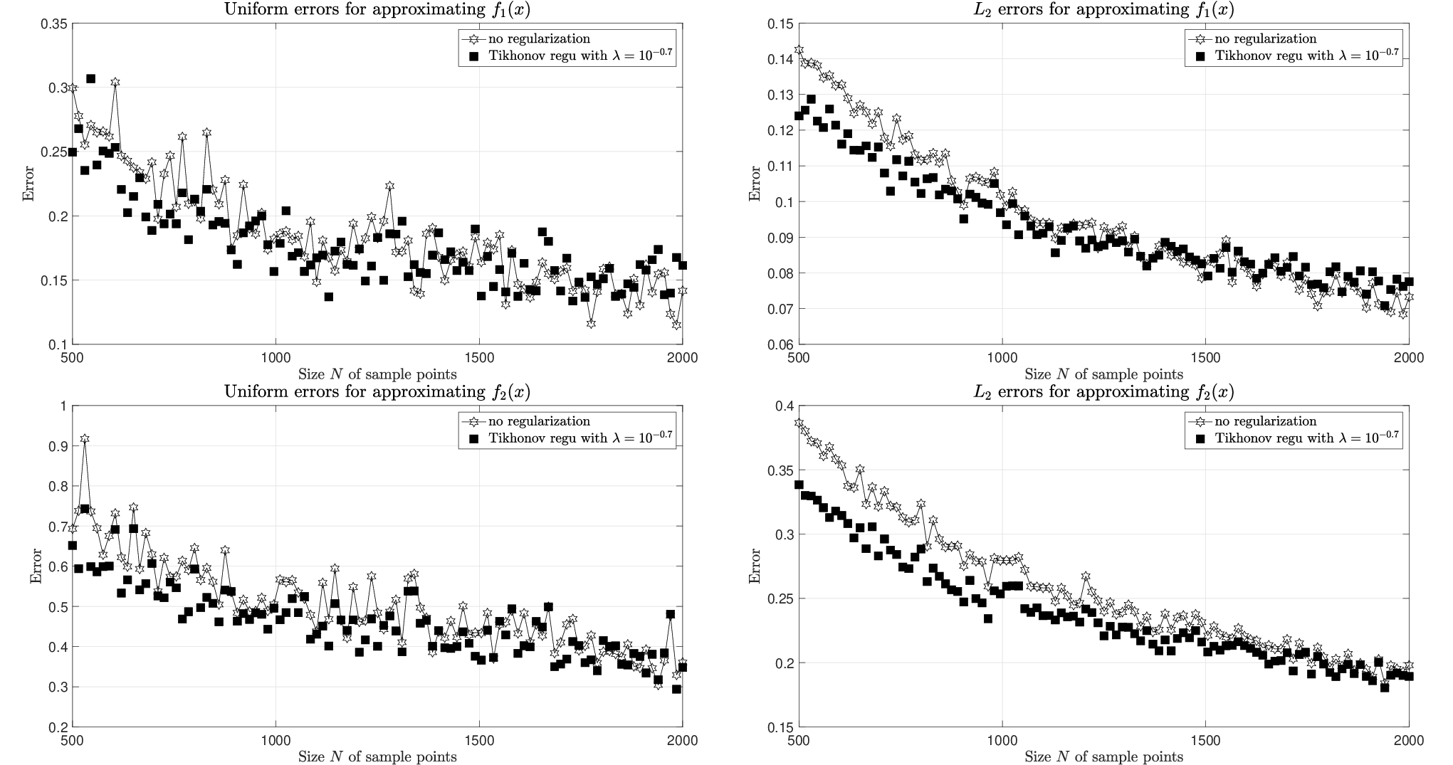
On the other hand, if we fix and let be increasing from to , that is, data size is increasing, then Figure 2 describes decreasing uniform errors and errors with respect to . The starting value of is 500 since Gauss quadrature would lose its exactness if . Computational results plotted in Figure 2 also assert that the Tikhonov regularization can reduce noise, especially when is small. In this case, the gap becomes narrow as increasing, which is due to the same fact that more data lead to better performance. This narrowing gap also indicates that Tikhonov regularization can handle this data shortage issue.
We then test the efficiency of Tikhonov regularized barycentric interpolation formula (3.8) in approximating , with data sampled on Gauss-Chebyshev points of the first kind. The experiment is conducted via the barycentric interpolation scheme (3.8) rather than the approximation scheme (2.5) under interpolatory conditions. Computational results in Figure 3 show that Tikhonov regularized barycentric interpolation works better than classical barycentric interpolation in the presence of noise. However, in the noise-free case, both kinds of errors for classical barycentric interpolation decline to 0 as increasing but those for Tikhonov regularized case do not. This misconvergence result of Tikhonov regularized barycentric interpolation, in another perspective, is a good agreement with the theoretical result that regularization would introduce an additional error into the error bound (4.5), and this error is around in this experiment.

At last, we take a certain , say , and test on function . Figure 4 reports the results, and “true data” in all subfigures denotes values of at Gauss-Chebyshev points of the first kind. When data is sampled via , that is, there is no noise in sampling, as shown in the above experiment, regularization is not needed. For numerical results on classical barycentric interpolation with true data, we refer to [1, 34]. When data is sampled via a multiple of , which is here, true data and Tikhonov regularized interpolant appear to be in a good agreement, which is due to with . We then test on different levels of additive random noise. Data are sampled via and , respectively, where , and is a random number in which is generated by MATLAB command rand(1). Tikhonov regularized barycentric formula performs better than the classical formula when the level of noise becomes large, especially near both endpoints.

If we add an oscillating term onto , plots in Figure 5 show the similar results with those in Figure 4. In this figure, Tikhonov regularized barycentric formula also performs better than the classical formula in concerned levels of noise, especially near extreme points of .

6 Concluding remarks
What we have seen from the above is that Tikhonov regularization can reduce noise in sampling data with an approximation scheme, in terms of reducing Lebesgue constants and the error term relating to noise. But it also introduces an additional error term, hence a trade-off strategy should be customized in practice. These findings also suit for the newly presented Tikhonov regularized barycentric formulae. While solving this approximation problem, it is shown that proper choice of orthonormal polynomials and Gauss quadrature points leads to entry-wise closed-form solutions to the problem, which simplifies the analysis on the approximation scheme. Gauss quadrature rules can be relaxed by using the concept of Marcinkiewicz-Zygmund quadrature measure (see, for example, [3, 19, 20, 22]), thus results in this paper can be generalized based on Marcinkiewicz-Zygmund quadrature. The reason why Gauss quadrature rules are adopted in this paper is two-fold: on the one hand, using Gauss quadrature is enough to provide a window into the behavior of approximation error in the usage of Tikhonov regularization and in the presence of noise; on the other hand, the development of barycentric interpolation formulae is based on Gauss quadrature points [1].
Although we only consider the simplest Tihonov regularization term, it also provides some useful information that regularization may improve performance of polynomial approximation. In inverse problems, statistics, and machine learning, different kinds of regularization terms are developed. We may consider other regularization techniques and derive other regularized barycentric interpolation formulae in the future. With the fast and stable property of barycentric formulae, regularized barycentric formulae provide a flexible choice for polynomial interpolation in noisy case, which only introduces a multiplicative factor or maybe other corrective factors derived in the future. Last but far from the least, the choices of the polynomial degree and regularization parameter deserve future studies. The polynomial degree has already been considered as a regularization parameter to deal with ill-conditioned issues [12, 21, 23, 24], and we expect an appropriate choice of to make better performance in the context of Tikhonov regularized polynomial approximation. Regularization parameter , which is chosen in a manual way in numerical experiments, also needs to be addressed more adaptively, see, for example, [10, 16, 25].
Acknowledgment
The authors are greatly thankful to the anonymous referees for valuable suggestions that helped to improve this paper.
References
References
- [1] Berrut, J.-P., and Trefethen, L. N. Barycentric Lagrange interpolation. SIAM Review 46, 3 (2004), 501–517.
- [2] Driscoll, T. A., Hale, N., and Trefethen, L. N. Chebfun Guide. Pafnuty Publications, Oxford, 2014.
- [3] Filbir, F., and Mhaskar, H. N. Marcinkiewicz–Zygmund measures on manifolds. Journal of Complexity 27, 6 (2011), 568–596.
- [4] Gautschi, W. Orthogonal Polynomials: Computation and Approximation. Oxford University Press, Oxford, 2004.
- [5] Gautschi, W. Numerical analysis 2nd edition. Birkhäuser, Basel, 2012.
- [6] Glaser, A., Liu, X., and Rokhlin, V. A fast algorithm for the calculation of the roots of special functions. SIAM Journal on Scientific Computing 29, 4 (2007), 1420–1438.
- [7] Hesse, K., Sloan, I. H., and Womersley, R. S. Radial basis function approximation of noisy scattered data on the sphere. Numerische Mathematik 137, 3 (2017), 579–605.
- [8] Higham, N. J. The numerical stability of barycentric Lagrange interpolation. IMA Journal of Numerical Analysis 24, 4 (2004), 547–556.
- [9] Kress, R. Numerical analysis, vol. 181 of Graduate Texts in Mathematics. Springer, New York, 1998.
- [10] Lazarov, R. D., Lu, S., and Pereverzev, S. V. On the balancing principle for some problems of numerical analysis. Numerische Mathematik 106, 4 (2007), 659–689.
- [11] Le Gia, Q. T., and Mhaskar, H. N. Localized linear polynomial operators and quadrature formulas on the sphere. SIAM Journal on Numerical Analysis (2008), 440–466.
- [12] Lu, S., Naumova, V., and Pereverzev, S. V. Legendre polynomials as a recommended basis for numerical differentiation in the presence of stochastic white noise. Journal of Inverse and Ill-posed Problems 21, 2 (2013), 193–216.
- [13] Lu, S., and Pereverzev, S. V. Sparse recovery by the standard Tikhonov method. Numerische Mathematik 112, 3 (2009), 403–424.
- [14] Lu, S., and Pereverzev, S. V. Regularization theory for ill-posed problems: Selected topics, vol. 58. De Gruyter, Berlin, 2013.
- [15] Lu, S., Pereverzev, S. V., and Ramlau, R. An analysis of Tikhonov regularization for nonlinear ill-posed problems under a general smoothness assumption. Inverse Problems 23, 1 (2006), 217.
- [16] Lu, S., Pereverzev, S. V., Shao, Y., and Tautenhahn, U. Discrepancy curves for multi-parameter regularization. Journal of Inverse and Ill-posed Problems 18, 6 (2010), 655–676.
- [17] Lu, S., Pereverzev, S. V., and Tautenhahn, U. A model function method in regularized total least squares. Applicable Analysis 89, 11 (2010), 1693–1703.
- [18] Lu, S., Pereverzev, S. V., and Tautenhahn, U. Regularized total least squares: Computational aspects and error bounds. SIAM Journal on Matrix Analysis and Applications 31, 3 (2010), 918–941.
- [19] Mhaskar, H. N. Polynomial operators and local smoothness classes on the unit interval. Journal of Approximation Theory 131, 2 (2004), 243–267.
- [20] Mhaskar, H. N. Polynomial operators and local smoothness classes on the unit interval, ii. Jaen Journal on Approximation Theorem 1 (2005), 1–25.
- [21] Mhaskar, H. N. A direct approach for function approximation on data defined manifolds. Neural Networks 132 (2020), 253–268.
- [22] Mhaskar, H. N., Narcowich, F. J., and Ward, J. D. Spherical Marcinkiewicz–Zygmund inequalities and positive quadrature. Mathematics of Computation 70, 235 (2001), 1113–1130.
- [23] Mhaskar, H. N., Naumova, V., and Pereverzyev, S. V. Filtered Legendre expansion method for numerical differentiation at the boundary point with application to blood glucose predictions. Applied Mathematics and Computation 224 (2013), 835–847.
- [24] Mhaskar, H. N., Pereverzyev, S. V., and van der Walt, M. D. A deep learning approach to diabetic blood glucose prediction. Frontiers in Applied Mathematics and Statistics 3 (2017), 14.
- [25] Pereverzyev, S. V., Sloan, I. H., and Tkachenko, P. Parameter choice strategies for least-squares approximation of noisy smooth functions on the sphere. SIAM Journal on Numerical Analysis 53, 2 (2015), 820–835.
- [26] Rivlin, T. J. An introduction to the approximation of functions. Blaisdell, Waltham, Massachusetts, 1969.
- [27] Rutishauser, H. Lectures on numerical mathematics. Birkhäuser, Berlin, 1990.
- [28] Salzer, H. E. Lagrangian interpolation at the Chebyshev points , ; some unnoted advantages. The Computer Journal 15, 2 (1972), 156–159.
- [29] Schwarz, H. R., and Waldvogel, J. Numerical analysis: a comprehensive introduction. Wiley, New York, 1989.
- [30] Sloan, I. H. Polynomial interpolation and hyperinterpolation over general regions. Journal of Approximation Theory 83, 2 (1995), 238–254.
- [31] Szegő, G. Orthogonal polynomials, vol. 23 of Colloquium Publications Volume XXIII. American Mathematical Society, Providence, Rhode Island, 1939.
- [32] Tikhonov, A. N., and Arsenin, V. J. Solutions of ill-posed problems. Winston & Sons, Washington, D.C., 1977.
- [33] Trefethen, L. N. Approximation theory and approximation practice, vol. 128. SIAM, Philadelphia, 2013.
- [34] Wang, H., Huybrechs, D., and Vandewalle, S. Explicit barycentric weights for polynomial interpolation in the roots or extrema of classical orthogonal polynomials. Mathematics of Computation 83, 290 (2014), 2893–2914.
- [35] Wang, H., and Xiang, S. On the convergence rates of Legendre approximation. Mathematics of Computation 81, 278 (2012), 861–877.
- [36] Wei, Y., Xie, P., and Zhang, L. Tikhonov regularization and randomized GSVD. SIAM Journal on Matrix Analysis and Applications 37, 2 (2016), 649–675.
- [37] Xiang, H., and Zou, J. Regularization with randomized SVD for large-scale discrete inverse problems. Inverse Problems 29, 8 (2013), 085008.
- [38] Xiang, H., and Zou, J. Randomized algorithms for large-scale inverse problems with general Tikhonov regularizations. Inverse Problems 31, 8 (2015), 24.
- [39] Xiang, S. On error bounds for orthogonal polynomial expansions and Gauss-type quadrature. SIAM Journal on Numerical Analysis 50, 3 (2012), 1240–1263.
- [40] Zhong, M., Lu, S., and Cheng, J. Multiscale analysis for ill-posed problems with semi-discrete tikhonov regularization. Inverse Problems 28, 6 (2012), 065019.