Testing error distribution by kernelized Stein discrepancy in multivariate time series models
Knowing the error distribution is important in many multivariate time series applications. To alleviate the risk of error distribution mis-specification, testing methodologies are needed to detect whether the chosen error distribution is correct. However, the majority of the existing tests only deal with the multivariate normal distribution for some special multivariate time series models, and they thus can not be used to testing for the often observed heavy-tailed and skewed error distributions in applications. In this paper, we construct a new consistent test for general multivariate time series models, based on the kernelized Stein discrepancy. To account for the estimation uncertainty and unobserved initial values, a bootstrap method is provided to calculate the critical values. Our new test is easy-to-implement for a large scope of multivariate error distributions, and its importance is illustrated by simulated and real data.
Keywords and phrases: Consistent test; Kernelized Stein discrepancy; Multivariate time series model; Testing multivariate error distribution.
1 Introduction
Consider a multivariate stationary time series with , and admits the following specification
| (1.1) |
where is the information set up to time , is the true yet unknown model parameter, is a sequence of independent and identically distributed (i.i.d.) errors with zero mean and identity covariance matrix , is a known measurable vector function indexed by , and is a known measurable symmetric and positive definite matrix function indexed by . Let be a sigma-field generated by . Conditional on , and in (1.1) are the conditional mean vector and conditional covariance matrix of , respectively. The general specification in (1.1) covers many often used multivariate models including, for example, the vector autoregressive and moving-average (VARMA) model, the multivariate generalized autoregressive conditional heteroskedasticity (MGARCH) model, and their variants and combinations. For surveys on the multivariate time series models, we refer to Lütkepohl (2005), Bauwens et al. (2006), Tsay (2013), and Francq and Zakoïan (2019).
For model (1.1), is assumed to have certain continuous probability density function (p.d.f.) in a myriad of applications, which include the validity of capital asset pricing model (Berk, 1997), the optimal forecasts (Christoffersen and Diebold, 1997), the density forecasts (Diebold et al., 1998), the interval forecasts (Zhu and Li, 2015), the option pricing (Zhu and Ling, 2015), and the Value-at-Risk and Expected Shortfall calculations (Taylor, 2019). However, the true p.d.f. of , denoted by , is generally unknown in practice, and the empirical researchers could make wrong conclusions if their assumed p.d.f. is different from . Motivated by this, it is important to testing for the following hypotheses
| (1.2) |
Our considered hypotheses in (1.2) are designed for the unobserved model error , which nests the observed data (i.e., ) as a special case. In this paper, we mainly focus on the testing for unobserved , and the testing methodologies for univariate/multivariate observed time series can be found in Lobato and Velasco (2004), Bai and Ng (2005), Mecklin and Mundfrom (2004), Székely and Rizzo (2005), and the references therein.
Since is unobserved, one need use the model residual to form valid tests for the hypotheses in (1.2). When is univariate (i.e., ), a number of different testing methods were proposed in the literature. Bontemps and Meddahi (2005) considered the robust moment tests for normality of by using the Hermite polynomials, and their idea was further extended in Bontemps and Meddahi (2012) to examine the general distribution of . Although these robust moment tests are easy-to-implement with a chi-square limiting null distribution, they are inconsistent as only a finite number of moments of are considered for the testing purpose. To construct consistent tests, other strategies have been adopted. For the general model as in (1.1), Bai (2003) developed Kolmogorov–Smirnov (KS) and Cramér–von Mises (CvM) tests by measuring the distance between the empirical distribution of and the cumulative distribution of . For the GARCH model, Horváth and Zitikis (2006) gave a smooth-type test by measuring the distance between the kernel density estimator of and the assumed density in -norm with , and Klar et al. (2012) constructed an integrated test by measuring the distance between the empirical characteristic function of and the characteristic function of . For the ARMA–GARCH model, Koul and Ling (2006) studied a weighted KS test based on a vector of certain weighted residual empirical processes.
When is multivariate (i.e., ) and both and are constants, most of earlier efforts were made to detect the normality of . See, for example, Mardia (1974), Henze and Zirkler (1990), Doornik and Hansen (2008), and references therein. When is multivariate but either or is non-constant, only few testing methods were provided for the MGARCH model. For instance, Bai and Chen (2008) applied a similar idea as Bai (2003) to propose consistent KS tests for detecting the multivariate normal and distributions of . Their tests are asymptotically distribution-free, however, they are not fully consistent and require the explicit form of the conditional cumulative distribution function of (conditional on ), which is neither available for other multivariate distributions, nor easily computable for the dimension . Francq et al. (2017) developed KS and CvM tests to examine whether has the elliptic distribution by extending the idea of Henze et al. (2014). These KS and CvM tests are not asymptotically distribution-free, and their application scope could be narrowed down when detecting the exact distribution of is needed. Henze et al. (2019) constructed consistent tests for the normality of by using the identity
| (1.3) |
where is the real part of , is the characteristic function of , and is the moment generating function of . Since the identity above only holds for multivariate normal distributions, their idea can not be extended to testing for other distributions. In economic and financial applications, many heavy-tailed or skewed error distributions could outperform the multivariate normal or distribution (see, e.g., Haas et al. (2004), Bauwens and Laurent (2005), De Luca et al. (2006), and references therein). Hence, it is necessary to construct a valid test for detecting the general multivariate distribution of in model (1.1).
This paper is motivated to propose a new consistent test for based on the kernelized Stein discrepancy (KSD) in Liu et al. (2016). The KSD measures the distance between the (Stein) score functions of and under the norm induced by a kernel function. For the observed data , Liu et al. (2016) constructed a test statistic for , and established its asymptotics. However, when is replaced by , we find that their results are not applicable any more due to the estimation effect in . To handle the estimation effect, our new KSD-based test is constructed based on a subsample of . Under certain conditions, we show that our test has no estimation effect, and establish its asymptotics under and . Although the estimation effect is negligible in theory, it may still exist in finite samples especially when the sample size is small. To overcome this difficulty, we introduce a simple parametric bootstrap method to calculate the critical values of our test. Simulations show that our test performs well in the examined cases, even when no or few effective data are discarded by our subsampling technique. A real data analysis is further given to demonstrate the usefulness of our test.
The remaining paper is organized as follows. Section 2 introduces the KSD-based test statistic. Section 3 studies the asymptotics of the KSD-based test statistic and provides a parametric bootstrap method to calculate the critical values. Simulation results are reported in Section 4, and a real example is offered in Section 5. Concluding remarks are given in Section 6. Proofs are deferred into Appendices.
2 KSD-based test statistic
2.1 Preliminaries on the KSD
In this paper, we construct a new test for hypotheses in (1.2) based on the kernelized Stein discrepancy (KSD) in Liu et al. (2016). Let be the true p.d.f. of in (1.1) with the support . To introduce the KSD, we first need define the (Stein) score function of and the Stein class of .
DEFINIOTION 2.1.
The (Stein) score function of is defined as
DEFINIOTION 2.2.
A function is in the Stein class of if is continuous differential and satisfies
| (2.1) |
When , by using integration by parts, the condition (2.1) holds if
which holds, for example, if is bounded and .
Next, let be an integrally strictly positive definite kernel function, that is,
for any function satisfying . With the kernel function , we are ready to give the definition of KSD between the distributions of and .
DEFINIOTION 2.3.
The KSD is defined as
| (2.2) |
where is the score difference between and , and , are i.i.d. from .
Clearly, the KSD measures the difference between the (Stein) score functions of and under a norm induced by the kernel function . If and are continuous with , Liu et al. (2016) showed that and
| (2.3) |
In view of the result (2.3), we can detect the null hypothesis in (1.2) by examining whether is significantly different from zero. However, a direct testing implementation based on (2.2) is infeasible, since the score difference is unknown. To overcome this difficulty, we need an additional condition on the kernel function .
DEFINIOTION 2.4.
The kernel function is in the Stein class of if has continuous second order partial derivatives, and both and are in the Stein class of for any fixed .
2.2 The KSD-based test statistic
To form our test statistic, a sample counterpart of in (2.4), based on the model residuals, is needed. Let be the unknown parameter of model (1.1), where is compact parametric space. Assume that is an interior point of , and denote
| (2.5) |
By (2.5), the model residual in (1.1) can be computed as
| (2.6) |
where , containing possible given initial values, is the truncated information set at time , and is an estimator of . With model residuals , the KSD-based test statistic as the estimator of in (2.4) is given by
| (2.7) |
where for some . Clearly, is a U-statistic with kernel function , and the calculation of only requires the computation of , , , and , which does not raise any computational burden even for a large dimension . For the kernel function , the often used one is the Gaussian kernel
| (2.8) |
where is a fixed constant; in this case, we have
For the score function , we show how to calculate it for some well-known distributions.
EXAMPLE 2.1.
Let be the multivariate normal distribution in , where is the location vector, and is the scale matrix. When is , we have .
EXAMPLE 2.2.
Let be the multivariate distribution in , where is the location vector, is the scale matrix, and is the degrees of freedom. When is (denoted by ) with mean zero and covariance matrix , we have
EXAMPLE 2.3.
Let be the multivariate skew-normal distribution in (Arellano-Valle and Azzalini, 2008), where is the location vector, is the scale matrix, and is the shape vector. To make sure that has mean zero and covariance matrix , we can choose the skewness vector and then set
| (2.9) |
where , , , and with
Under the settings in (2.9), we denote as . When is with mean zero and covariance matrix , we have
where and denote the density and distribution functions, respectively.
Unlike Liu et al. (2016), our test statistic does not use the entire data . This is because we have to sacrifice some part of to deal with the effect of estimation uncertainty caused by replacing via and the effect of unobserved initial values resulting from substituting by . With the assist of bootstrap scheme, our numerical studies in Section 4 show that can have good a size and power performance even when no or few data are discarded. Hence, it suggests that can be used with or in practice, and the subsampling technique seems only theoretically relevant.
3 Asymptotic theory
3.1 Technical assumptions
Denote
where is defined in (2.5). In this subsection, we give some technical assumptions to study the asymptotics of .
ASSUMPTION 3.1.
is strictly stationary and ergodic.
ASSUMPTION 3.2.
.
ASSUMPTION 3.3.
The function satisfies that
(i) ;
(ii) ,
for any .
ASSUMPTION 3.4.
The estimator satisfies that .
ASSUMPTION 3.5.
The function satisfies that
ASSUMPTION 3.6.
The distributions and satisfy that
(i) both and are continuous with ;
(ii) , where is one of and , for any , and is a given constant.
ASSUMPTION 3.7.
The kernel function satisfies that
(i) is in the Stein class of ;
(ii) and its partial derivatives up to fourth order are all uniformly bounded.
A few remarks are in order related to the aforementioned assumptions. Assumptions 3.1–3.2 are regular in many time series applications. Assumption 3.3 poses some moment conditions on the derivatives of for the purpose of proof, and Assumption 3.4 holds for most estimators such as the least squares estimator (LSE) for VARMA models and the quasi-maximum likelihood estimator (QMLE) for VARMA–GARCH models. Sufficient conditions to validate Assumptions 3.3–3.4 can be found in Lütkepohl (2005) for VARMA models, Comte and Lieberman (2003), Hafner and Preminger (2009), and Francq and Zakoïan (2012) for MGARCH models, and Ling and McAleer (2003) for VARMA–MGARCH models. Assumption 3.5 is a condition on the approximation error by replacing the information set by , and it is used to show that the unobserved initial values have the negligible effect on the asymptotic theory. See also Hong and Lee (2005) and Escanciano (2006) for the similar conditions.
Assumption 3.6 requires both and to have certain smooth conditions. The condition is sufficient to prove the equivalence result (2.3). As argued in Liu et al. (2016), this condition is mild. For example, it holds when is the density function of multivariate normal and distributions or has an exponentially decayed tail, but it may not hold when has a heavy tail. Note that the exclusion of heavy-tailed is also implied by Assumption 3.2. Assumption 3.7(i) ensures the validity of (2.4), and Assumption 3.7(ii) poses some boundedness conditions on and its derivatives. It is easy to check that Gaussian kernel in (2.8) satisfies Assumption 3.7 for any smooth density supported on . Hence, we follow Liu et al. (2016) to use the Gaussian kernel in this paper.
3.2 Asymptotics of
According to Theorem 3.7 in Liu et al. (2016), the kernel function is positive definite, and then by Mercer’s theorem, admits the expansion
| (3.1) |
where and are the orthonormal eigenfunctions and eigenvalues of . We are ready to give the limiting null distribution of .
THEOREM 3.1.
Our limiting null distribution in Theorem 3.1 is the same as the one in Theorem 4.1 of Liu et al. (2016), since the effects of estimation uncertainty and unobserved initial values are asymptotically negligible by using the sub-sample technique with . When , how to establish the limiting null distribution of is unclear at this stage, and we leave this topic for future study.
Although the effects of estimation uncertainty and unobserved initial values are asymptotically negligible in theory, they may exist in finite samples especially when is small. To redeem this drawback, we propose a simple parametric bootstrap method in Subsection 3.3 below to calculate the critical values of . Owing to the use of bootstrap, our simulation studies will show that has a good finite-sample performance even for very small value of , indicating that the condition should not be an obstacle for applications.
Next, the behavior of under is given in the following theorem.
Let be the critical value of at the level . Then, the preceding theorem implies that under , the power function converges to 1 as , and hence can detect consistently.
To end this subsection, we discuss how the choice of in (2.8) affects the value of . By (A.15) in Appendix A.2, we can show that under , for large ,
| (3.2) |
To further calculate , we assume (as recommended for practical use) and
as , where is the asymptotic covariance matrix. Then, by (3.2) it is straightforward to see
| (3.3) |
where , and is the limit of by the law of large numbers for U-statistics. From (3.3), we know that should be chosen such that is maximized. However, this implementation can not be accomplished in an easy way, since an explicit form of is not available. Therefore, it seems hard to choose optimally. In practice, we can follow Liu et al. (2016) to choose as the median of residual distance:
| (3.4) |
where . Our simulation studies in Section 4 below show that has a good finite-sample performance based on this choice of .
3.3 The computation of critical values
When is observed (i.e., ), Liu et al. (2016) applied a Wild bootstrap method to calculate critical values for their test. However, when is unobserved as in our settings, their bootstrap scheme may not work, since it does not account for the effects of estimation uncertainty and unobserved initial values, which can affect our critical value in the finite sample. In this paper, we apply the following parametric bootstrap method to calculate :
Step 1. Draw bootstrap i.i.d. errors and calculate the bootstrap data sample
where is the bootstrap counterpart of .
Step 2. Calculate the bootstrap estimator and the bootstrap residuals
where is the bootstrap counterpart of .
Step 3. Compute the bootstrap test statistic , based on the bootstrap residuals.
Step 4. Repeat steps 1–3 times to get , whose empirical upper quantile is taken as the critical value .
4 Simulations
In this section, we carry out simulation experiments to assess the performance of our KSD-based test in finite samples. For the purpose of comparison, some widely-used tests (see Appendix A.3 for their definitions and asymptotics) are also considered. The data generating processes (DGPs) considered below cover the dimension and . In all simulations, we take the sample size or , choose the number of repetitions , and set the significance level , 5%, or 10%. For , we use the Gaussian kernel in (2.8) with taken as in (3.4), and choose such that no data are discarded. To reduce the computational burden in simulations, we follow Francq et al. (2017) to adopt the Warp-Speed method of Giacomini et al. (2013) for evaluating the bootstrap scheme proposed in Subsection 3.3. With the Warp-Speed method, rather than computing critical value for each repetition sample, only one resample is generated for each repetition sample and the resampling test statistic is computed for that sample. Then the critical value is computed from the empirical distribution determined by the resampling repetitions .
4.1 Case 1: Constant mean and constant covariance models
We consider the DGP given by a constant mean and constant covariance model
| (4.1) |
where and are constant mean and constant covariance of , respectively, and they are chosen as
for , and
for . In model (4.1), the distribution of (i.e., the true distribution ) is , , , or , where the first three distributions are given in Examples 2.1–2.3, and the fourth distribution is the multivariate skew- distribution in Bauwens and Laurent (2005) with mean zero, covariance matrix , being the degrees of freedom, and being the asymmetry vector to control the skewness. In the sequel, we set
| Test | 1% | 5% | 10% | 1% | 5% | 10% | 1% | 5% | 10% | 1% | 5% | 10% | ||
| 100 | 0.6 | 5.5 | 11.5 | 61.0 | 75.9 | 84.1 | 16.8 | 34.5 | 46.3 | 80.7 | 88.9 | 95.2 | ||
| 0.7 | 4.6 | 9.5 | 53.3 | 65.5 | 72.0 | 25.7 | 47.0 | 61.1 | 67.4 | 81.9 | 89.3 | |||
| 1.4 | 3.2 | 6.9 | 80.6 | 87.3 | 90.6 | 9.1 | 13.1 | 17.0 | 93.4 | 96.0 | 98.8 | |||
| 1.5 | 5.5 | 10.0 | 70.9 | 82.5 | 87.2 | 24.3 | 42.5 | 53.3 | 84.7 | 91.5 | 96.6 | |||
| 0.5 | 5.4 | 11.0 | 48.1 | 66.1 | 75.7 | 9.9 | 26.5 | 38.7 | 73.1 | 84.9 | 92.1 | |||
| 9.3 | 15.5 | 22.7 | 49.7 | 64.2 | 71.5 | 0.2 | 1.4 | 3.3 | 70.3 | 79.4 | 88.2 | |||
| 12.0 | 21.8 | 29.4 | 51.8 | 66.8 | 73.2 | 0.2 | 2.4 | 4.8 | 72.5 | 82.0 | 89.3 | |||
| 11.8 | 19.6 | 27.4 | 53.2 | 66.5 | 74.9 | 0.2 | 1.9 | 5.6 | 73.1 | 84.5 | 90.7 | |||
| 0.8 | 5.7 | 11.2 | 56.1 | 68.4 | 77.4 | 4.5 | 12.4 | 20.1 | 75.0 | 86.2 | 92.8 | |||
| 500 | 1.3 | 5.3 | 9.6 | 100 | 100 | 100 | 91.9 | 98.2 | 99.1 | 100 | 100 | 100 | ||
| 1.2 | 5.6 | 10.1 | 78.4 | 86.1 | 89.6 | 99.0 | 99.9 | 100 | 100 | 100 | 100 | |||
| 1.4 | 4.0 | 8.3 | 100 | 100 | 100 | 23.4 | 36.2 | 43.9 | 100 | 100 | 100 | |||
| 1.2 | 4.0 | 9.5 | 99.9 | 100 | 100 | 98.7 | 99.8 | 99.9 | 100 | 100 | 100 | |||
| 0.9 | 4.9 | 9.2 | 99.7 | 100 | 100 | 71.6 | 87.4 | 92.7 | 100 | 100 | 100 | |||
| 8.8 | 14.6 | 23.1 | 88.3 | 93.5 | 97.6 | 0.3 | 2.7 | 10.2 | 100 | 100 | 100 | |||
| 13.2 | 23.5 | 31.7 | 91.2 | 94.1 | 98.2 | 0.6 | 4.5 | 16.4 | 100 | 100 | 100 | |||
| 12.6 | 21.4 | 28.9 | 91.7 | 96.0 | 99.2 | 2.0 | 8.1 | 18.1 | 100 | 100 | 100 | |||
| 1.2 | 4.8 | 9.5 | 100 | 100 | 100 | 13.8 | 30.4 | 41.7 | 100 | 100 | 100 | |||
| 100 | 0.4 | 9.4 | 25 | 0.5 | 4.9 | 9.4 | 2 | 26.6 | 48.8 | 4.4 | 20.6 | 33.6 | ||
| 0 | 0 | 0 | 8.5 | 14.2 | 20.1 | 0 | 0 | 4.6 | 2.9 | 9.6 | 18.8 | |||
| 0 | 0 | 0 | 13.5 | 23.7 | 30.6 | 2.3 | 4.1 | 5.3 | 3.6 | 11.2 | 17.7 | |||
| 0 | 0 | 0 | 11.7 | 21.9 | 28.6 | 1.8 | 2.3 | 3.7 | 4.4 | 11.3 | 18.9 | |||
| 500 | 81.8 | 99.5 | 100 | 0.4 | 4.6 | 10.5 | 99.4 | 100 | 100 | 90.6 | 100 | 100 | ||
| 0 | 0 | 0.4 | 7.8 | 14.5 | 22.7 | 0.5 | 4.3 | 12.1 | 77.3 | 96.3 | 100 | |||
| 0 | 0.1 | 1.1 | 13.1 | 23.6 | 31.5 | 1.4 | 6.7 | 16.8 | 79.1 | 96.9 | 100 | |||
| 0 | 0 | 0.8 | 12.2 | 20.4 | 30.2 | 1.4 | 7.1 | 18.5 | 80.7 | 98.5 | 100 | |||
| 100 | 14.9 | 32.5 | 45.1 | 73.6 | 87.7 | 91.9 | 0.9 | 5.0 | 10.2 | 94.6 | 98.0 | 98.7 | ||
| 500 | 95.9 | 99.3 | 99.9 | 100 | 100 | 100 | 0.5 | 3.9 | 8.4 | 100 | 100 | 100 | ||
| ) | ||||||||||||||
| Test | 1% | 5% | 10% | 1% | 5% | 10% | 1% | 5% | 10% | 1% | 5% | 10% | ||
| 100 | 1.4 | 4.8 | 9.7 | 97.9 | 99.5 | 99.9 | 17.0 | 38.5 | 52.3 | 100 | 100 | 100 | ||
| 1.1 | 4.7 | 8.4 | 95.2 | 97.3 | 98.4 | 3.2 | 10.9 | 16.7 | 100 | 100 | 100 | |||
| 0.5 | 2.7 | 8.5 | 99.5 | 100 | 100 | 3.8 | 7.3 | 10.5 | 100 | 100 | 100 | |||
| 1.6 | 5.1 | 9.7 | 90.8 | 95.6 | 97.3 | 3.3 | 10.8 | 18.2 | 100 | 100 | 100 | |||
| 0.8 | 4.8 | 11 | 92.9 | 96.4 | 98 | 7.8 | 20.7 | 30.5 | 100 | 100 | 100 | |||
| 1.4 | 5.2 | 10.4 | 94.3 | 98.7 | 99.3 | 3.2 | 10.1 | 17.4 | 100 | 100 | 100 | |||
| 500 | 1.5 | 5.0 | 9.3 | 100 | 100 | 100 | 99.1 | 99.9 | 100 | 100 | 100 | 100 | ||
| 1.1 | 4.8 | 10.2 | 100 | 100 | 100 | 27.9 | 50.0 | 64.0 | 100 | 100 | 100 | |||
| 0.4 | 4.4 | 8.4 | 100 | 100 | 100 | 5.3 | 10.6 | 16.6 | 100 | 100 | 100 | |||
| 1.3 | 5.1 | 9.7 | 100 | 100 | 100 | 19.5 | 38.1 | 50.8 | 100 | 100 | 100 | |||
| 1.0 | 5.0 | 8.2 | 100 | 100 | 100 | 72.1 | 89.3 | 93.6 | 100 | 100 | 100 | |||
| 1.4 | 5.2 | 8.9 | 100 | 100 | 100 | 9.0 | 22.9 | 33.8 | 100 | 100 | 100 | |||
| 100 | 4.2 | 15.8 | 38.1 | 1.3 | 4.9 | 9.8 | 0 | 0.1 | 0.4 | 26.8 | 50.3 | 64.9 | ||
| 500 | 87.3 | 100 | 100 | 1.0 | 4.7 | 10.2 | 75.3 | 100 | 100 | 100 | 100 | 100 | ||
| 100 | 60.9 | 75.1 | 80.5 | 89.5 | 96.7 | 98.5 | 1.0 | 4.2 | 8.7 | 99.2 | 99.8 | 99.9 | ||
| 500 | 100 | 100 | 100 | 100 | 100 | 100 | 1.1 | 4.9 | 9.7 | 100 | 100 | 100 | ||
For the null distribution in (1.2), we take it to be , , or . When is , we also consider Mardia’s skewness test (), Mardia’s kurtosis test (), Doornik–Hansen test (), Henze–Zirkler test (), Bai–Chen tests (, , and ), and Henze–Jiménez-Gamero–Meintanis test (). The first four tests , , , and are based on either the sample skewness or the sample kurtosis or both. The tests , , are based on the empirical distribution of the residuals, and the test is based on the characteristic function of the residuals. Note that except , all other tests work for . When is or , none of the competitive tests above is applicable, except that the tests can be used for the case of .
Tables 1 and 2 report the size and power of all examined tests for and , respectively, where the size corresponds to the case of . In calculation of , , and , the residuals of model (4.1) are computed by estimating and by the sample mean and sample covariance of , respectively. Note that since the tests are largely over-sized, we compute their size-adjusted power in the sequel. From Tables 1 and 2, our findings are as follows:
(1) Except for the tests , all examined tests have an accurate size performance at three levels.
(2) When is , has a comparative power performance with any competitive test to detect the alternative hypotheses that are and . However, has the best power performance to detect the alternative hypothesis that is , and the tests , , and have a much worse power performance in this case. The advantage of is more obvious for the case .
(3) When is , has the satisfactory power performance especially for , while the tests only exhibit the power to detect the alternative hypothesis that is .
(4) When is , is powerful to detect each examined alternative hypothesis, and its power to detect the heavy-tailed alternative distribution (e.g., or ) is higher than that to detect the light-tailed alternative distribution (e.g., ).
Overall, our KSD-based test exhibits the good size and power performance in all examined cases. All skewness- or kurtosis-based tests for normality generally perform well, except that lacks the power to detect the alternative distribution . The tests have the over-sized problem in all examined cases, and their size-adjusted power in general is not satisfactory especially for the null distribution . The test for the normality performs as good as , except that its power to detect the alternative distribution is lower. Based on the aforementioned findings, it is reasonable to recommend for use due to its generality and desirable power performance.
4.2 Case 2: VAR models
We consider the DGP given by a VAR(3) model
| (4.2) |
where , , and are chosen as in model (4.1), and
for , and
for . As in Case 1, the null distribution is , , or . For the VAR(3) model in (4.2), the skewness- or kurtosis-based tests considered in Case 1 are not applicable any more. In this case, the tests work when is or for , and the test works when is for and 5.
Tables 3 and 4 report the size and power of all examined tests for and , respectively, where the size corresponds to the case of . In calculation of , , and , the residuals of model (4.2) are computed by using the LSE to estimate the unknown parameters. From Tables 3 and 4, our findings are similar as those in Case 1.
| Test | 1% | 5% | 10% | 1% | 5% | 10% | 1% | 5% | 10% | 1% | 5% | 10% | ||
| 100 | 1.7 | 5.7 | 10.1 | 52.3 | 70.4 | 78.6 | 11.4 | 28.9 | 40.2 | 61.5 | 77.3 | 87.2 | ||
| 7.3 | 12.6 | 18.7 | 43.6 | 56.8 | 64.2 | 0 | 0.7 | 2.1 | 47.2 | 63.3 | 71.6 | |||
| 11.8 | 19.5 | 26.1 | 46.2 | 57.4 | 68.2 | 0 | 1.5 | 3.6 | 50.2 | 62.9 | 77.5 | |||
| 11.4 | 20.7 | 25.0 | 46.9 | 59.0 | 69.3 | 0 | 1.2 | 3.8 | 51.0 | 65.2 | 79.3 | |||
| 0.5 | 4.1 | 11.3 | 55.0 | 64.7 | 72.5 | 3.9 | 12.5 | 20.5 | 58.3 | 71.8 | 84.9 | |||
| 500 | 0.6 | 4.4 | 9.5 | 99.9 | 100 | 100 | 91.2 | 97.4 | 98.6 | 100 | 100 | 100 | ||
| 8.5 | 13.2 | 19.0 | 85.2 | 90.4 | 98.4 | 0.2 | 2.4 | 10.5 | 100 | 100 | 100 | |||
| 13.5 | 22.2 | 28.5 | 86.0 | 93.1 | 99.0 | 0.6 | 4.1 | 15.7 | 100 | 100 | 100 | |||
| 11.7 | 19.4 | 26.1 | 88.2 | 93.8 | 99.3 | 1.8 | 8.0 | 17.5 | 100 | 100 | 100 | |||
| 0.8 | 5.4 | 10.4 | 100 | 100 | 100 | 13.0 | 29.9 | 41.5 | 100 | 100 | 100 | |||
| 100 | 0.2 | 11.1 | 26.9 | 0.8 | 5.7 | 11.0 | 1.6 | 23.7 | 45.9 | 3.7 | 16.6 | 26.1 | ||
| 0 | 0.2 | 0.2 | 9.4 | 15.7 | 23.2 | 0.5 | 1.4 | 3.5 | 3.4 | 7.8 | 14.8 | |||
| 0 | 0.3 | 0.4 | 12.4 | 24.0 | 33.5 | 1.7 | 3.8 | 4.9 | 4.2 | 8.3 | 13.1 | |||
| 0 | 0.3 | 0.4 | 10.9 | 21.6 | 30.6 | 1.1 | 2.4 | 3.7 | 4.6 | 8.2 | 15.7 | |||
| 500 | 88.0 | 99.3 | 99.9 | 0.7 | 4.8 | 9.9 | 98.1 | 99.4 | 100 | 84.4 | 95.1 | 99.7 | ||
| 0 | 0 | 0.6 | 8.9 | 14.1 | 20.4 | 0.7 | 3.9 | 11.4 | 63.9 | 75.5 | 84.5 | |||
| 0 | 0.4 | 1.4 | 12.7 | 21.5 | 29.3 | 1.5 | 5.8 | 16.2 | 65.3 | 74.1 | 85.9 | |||
| 0 | 0.4 | 1.2 | 11.4 | 18.6 | 26.7 | 1.4 | 6.5 | 17.5 | 66.0 | 78.2 | 89.3 | |||
| 100 | 14.8 | 34.4 | 45.3 | 67.4 | 81.5 | 88.3 | 1.0 | 6.1 | 9.9 | 90.7 | 95.2 | 98.1 | ||
| 500 | 95.4 | 99.2 | 100 | 100 | 100 | 100 | 0.8 | 5.3 | 9.8 | 100 | 100 | 100 | ||
| Test | 1% | 5% | 10% | 1% | 5% | 10% | 1% | 5% | 10% | 1% | 5% | 10% | ||
| 100 | 1.1 | 4.8 | 9.6 | 89.4 | 96.7 | 99.1 | 12.1 | 29.7 | 42.1 | 98.4 | 100 | 100 | ||
| 0.6 | 4.7 | 10.3 | .0 | 95.2 | 98.3 | 3.7 | 11.8 | 18.9 | 97.7 | 99.7 | 100 | |||
| 500 | 1.3 | 5.2 | 10.7 | 100 | 100 | 100 | 98.5 | 99.6 | 100 | 100 | 100 | 100 | ||
| 0.9 | 4.7 | 9.2 | 100 | 100 | 100 | 9.3 | 23.4 | 32.8 | 100 | 100 | 100 | |||
| 100 | 2.7 | 11.8 | 36.4 | 1.4 | 6.2 | 10.5 | 0 | 0.2 | 0.6 | 25.3 | 48.2 | 59.7 | ||
| 500 | 100 | 100 | 100 | 1.4 | 5.7 | 11.1 | 72.8 | 99.2 | 100 | 100 | 100 | 100 | ||
| 100 | 58.4 | 73.8 | 78.8 | 84.7 | 91.4 | 95.3 | 0.7 | 4.5 | 10.4 | 95.8 | 98.5 | 99.7 | ||
| 500 | 100 | 100 | 100 | 100 | 100 | 100 | 0.9 | 5.8 | 10.3 | 100 | 100 | 100 | ||
4.3 Case 3: CCC–GARCH models
We consider the DGP given by a CCC-GARCH(1, 1) model
| (4.3) |
where is chosen as in model (4.1), and with
Here, the parameter matrices , , , and are set to be
for , and
for .
As in Cases 1 and 2, the null distribution is , , or . For the CCC-GARCH model in (4.3), the competitive tests can only be chosen as in Case 2. Tables 5 and 6 report the size and power of all examined tests for and , respectively, where the size corresponds to the case of . In calculation of , , and , the residuals of model (4.3) are computed by using the QMLE to estimate the unknown parameters. Clearly, our findings from Tables 5 and 6 are similar to those in Case 1.
| Test | 1% | 5% | 10% | 1% | 5% | 10% | 1% | 5% | 10% | 1% | 5% | 10% | ||
| 500 | 0.9 | 5.0 | 10.3 | 97.3 | 99.7 | 100 | 89.5 | 96.2 | 98.0 | 100 | 100 | 100 | ||
| 10.4 | 16.1 | 22.5 | 85.1 | 89.9 | 95.2 | 0 | 1.5 | 6.5 | 100 | 100 | 100 | |||
| 14.3 | 23.0 | 31.6 | 88.3 | 93.0 | 96.7 | 0.7 | 3.2 | 13.1 | 100 | 100 | 100 | |||
| 12.7 | 20.4 | 28.3 | 90.4 | 94.1 | 98.4 | 1.6 | 5.7 | 14.9 | 100 | 100 | 100 | |||
| 0.8 | 4.7 | 9.7 | 87.7 | 91.4 | 96.2 | 9.2 | 23.7 | 33.5 | 100 | 100 | 100 | |||
| 500 | 92.4 | 99.5 | 99.8 | 0.7 | 5.5 | 10.9 | 97.5 | 99.2 | 100 | 100 | 100 | 100 | ||
| 0 | 0 | 0.6 | 8.9 | 13.2 | 18.5 | 0.6 | 3.4 | 10.1 | 100 | 100 | 100 | |||
| 0.2 | 0.2 | 1.4 | 11.4 | 17.9 | 25.7 | 1.3 | 5.2 | 14.4 | 100 | 100 | 100 | |||
| 0.2 | 0.3 | 1.7 | 9.6 | 17.1 | 24.9 | 1.3 | 5.8 | 15.7 | 100 | 100 | 100 | |||
| 500 | 93.5 | 97.4 | 99.4 | 100 | 100 | 100 | 1.2 | 5.5 | 10.6 | 100 | 100 | 100 | ||
| Test | 1% | 5% | 10% | 1% | 5% | 10% | 1% | 5% | 10% | 1% | 5% | 10% | ||
|---|---|---|---|---|---|---|---|---|---|---|---|---|---|---|
| 500 | 1.3 | 5.6 | 11.2 | 100 | 100 | 100 | 96.8 | 98.3 | 99.7 | 100 | 100 | 100 | ||
| 0.7 | 4.6 | 9.5 | 100 | 100 | 100 | 8.5 | 22.8 | 30.6 | 100 | 100 | 100 | |||
| 500 | 100 | 100 | 100 | 1.2 | 5.1 | 10.4 | 68.7 | 98.4 | 100 | 100 | 100 | 100 | ||
| 500 | 100 | 100 | 100 | 100 | 100 | 100 | 1.3 | 4.8 | 10.5 | 100 | 100 | 100 | ||
4.4 Sensitivity analysis
In our previous simulation studies, we take and as in (3.4) to compute our KSD-based test . In this subsection, we implement the sensitivity analysis on the choice of or for , based on the DGP in (4.1) with being and being (for the size study) or (for the power study).
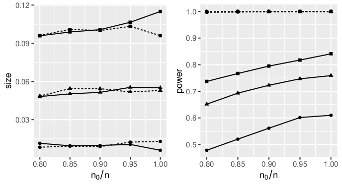
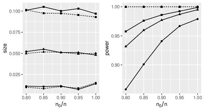
First, we consider the cases that is taken with the subsample ratio , , , and , while the value of is chosen as in (3.4). Fig 1 plots the size and power of across the subsample ratio . From this figure, we can find that (1) always has a good size performance; (2) when , the power of increases as the value of (or ) increases, and when , the power of reaches one in all examined cases. Therefore, as expected, we should recommend to use for , although this choice of is inconsistent to our theoretical setting.
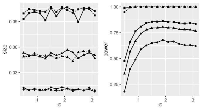
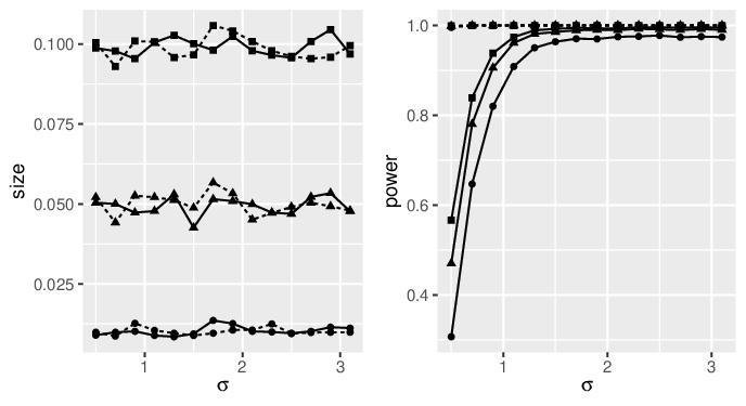
Second, we consider the cases that is set to be 0.5, 0.7, …, 3.1, while the value of is taken as . Fig 2 plots the size and power of across . From this figure, we can find that the size of is always accurate for each examined , and the power of for has only a marginal difference from that for the choice of in (3.4). These findings imply that tends to have a stable size and power performance over the choice of .
5 Application
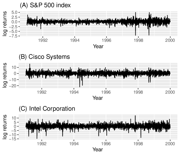
In this section, we revisit a real example in Tsay (2005). This example considered a three-dimensional financial time series, which consists of the daily log returns (in percentage) of the S&P 500 index, the stock price of Cisco Systems, and the stock price of Intel Corporation from January 2, 1991 to December 31, 1999, with 2275 observations in total. We denote this multivariate time series by , and plot each entry of in Fig 3. Following Tsay (2005), is fitted by a VAR(3)–CCC–GARCH(1, 1) model
| (5.1) |
with
For model (5.1), after dropping the insignificant parameters, we follow Tsay (2005) to first estimate the VAR(3) model by using the LSE, and then estimate the CCC–GARCH(1, 1) model by using the QMLE, where the resulting estimators are given by
Next, we use our KSD-based test to check the distribution of . The null distribution of interest is , , or , where the degrees of freedom is , 6, 7, 8, or 9, and the skewness vector is . Here, is the maximum likelihood estimator (MLE) of based on , and is the MLE of based on . To calculate , we choose and use the Gaussian kernel in (2.8) with taken as in (3.4). The p-value of is computed based on the parametric bootstrap in Subsection 3.3 with .
Table 7 reports the p-values of for all chosen null distributions . From this table, we can find that gives the strong evidence to reject the null distributions and , and on the contrary, it can not reject the null distributions , , , and at the significant level 5%. Since has the largest p-value for the null distribution , it is reasonable to conclude that in model (5.1) follows .
| p-value | 0.000 | 0.148 | 0.025 | 0.067 | 0.152 | 0.062 | 0.000 |
|---|
6 Concluding remarks
This paper constructed a new KSD-based test to detect the error distribution in multivariate time series models with general specifications. The KSD-based test is easy-to-implement as long as the (Stein) score function of the null distribution has an explicit form. Hence, it allows the null distribution of interest to be not only multivariate normal, but also multivariate , skew-normal, and many others. Since most of the existing tests only deal with the multivariate normal null distribution, the KSD-based test can largely broaden the testing scope for practitioners. This progress driven by the KSD-based test is important in view of the fact that the non-normal distributed errors are often recommended in various economic and financial applications.
Furthermore, our extensive simulation studies found that the KSD-based test not only shows its generality advantage to deal with multivariate non-normal null distributions, but also exhibits the comparative power with the existing tests to handle the multivariate normal null distribution. Finally, we studied a 3-dimensional financial time series by a VAR(3)–CCC–GARCH(1, 1) model, and the results of KSD-based test indicated that the error of this model follows a 3-dimensional multivariate distribution.
Appendices
A.1 The expansion of
To facilitate our proofs, we need a useful expansion of . First, we give some notation to present this expansion. Denote and
where
| (A.1) | ||||
| (A.2) |
Second, we define three U-statistics (for ) as follows:
| (A.3) |
where
with
With these notation, by Taylor’s expansion we have
| (A.4) |
where , lies between and , and
Furthermore, by Taylor’s expansion again we have
| (A.5) |
where lies between and , and
By (2.7) and (A.4)–(A.5), it follows that
| (A.6) |
where the U-statistics (for ) are defined in (A.3), and the remainder term is defined by
| (A.7) |
with and
From the expansion (A.6), it is clear that the estimation effect has an impact on the limiting distribution of through the linear term , the quadratic term , and the remainder term , and that the effect of unobserved initial values is involved in the remainder term via .
A.2 Proofs of Theorems 3.1–3.2
To prove Theorems 3.1–3.2, we need two technical lemmas to handle the effects of estimation uncertainty and unobserved initial values.
LEMMA A.1.
(i) , provided that ;
(ii) , provided that .
Proof of Lemma A.1. By Assumptions 3.1, 3.3, 3.6 and 3.7(ii) and the law of large numbers for U-statistics, it is not hard to see that and . Since by Assumption 3.4, it follows that and . Hence, the conclusions hold. ∎
Proof of Lemma A.2. For simplicity, we only show that
| (A.8) |
since the proof for is similar and even simpler. By (A.5), we can rewrite as
Then, it follows that , where
Let be a generic constant whose value may change from place to place. Next, we show that . To facilitate it, we claim
| (A.9) |
where holds uniformly in . With loss of generality, we prove (A.9) for , the first block entry of . Denote , where , , , and . Below, we first prove
| (A.10) |
Rewrite
Note that
| (A.11) | ||||
| (A.12) |
where in (A.11) holds uniformly in due to the fact that and by Assumptions 3.3(i) and 3.4, and (A.12) holds by Assumption 3.6. Therefore, by (A.11)–(A.12) and Assumption 3.7, the adding and subtracting arguments give us
Similarly, the same result holds for with Hence, the result (A.10) holds, and then we can show the same result for with Therefore, it entails that the result (A.9) holds.
Note that by Assumption 3.2, , and
by Assumption 3.5. Hence, by (A.9) and Hölder’s inequality, we can show
| (A.13) |
implying that .
Furthermore, by Taylor’s expansion, Assumptions 3.3–3.4, and a similar argument as for (A.11), it is straightforward to see
| (A.14) |
where holds uniformly in . By (A.14) and the similar arguments as for (A.13), we can show that for . Therefore, it follows that the result (A.8) holds. This completes the proof. ∎
A.3 Tests used in simulation studies
1. Mardia’s tests. Consider the null hypothesis that
| (A.16) |
Mardia (1974) detected in (A.16) by proposing the following two test statistics:
where , and and are the sample mean and variance of , respectively. The tests and make use of the multivariate extensions of skewness and kurtosis measures in Mardia (1970), and they have the following limiting null distributions
2. Doornik–Hansen test. Let and be the original sample skewness and kurtosis, where . Next, transform and into and , respectively, where
Here,
Based on and , Doornik and Hansen (2008) proposed the test statistic to detect in (A.16), where the limiting null distribution of is .
3. Henze–Zirkler test. To detect in (A.16), Henze and Zirkler (1990) proposed a test statistic given by
where is the squared Mahalanobis distance between and , and is the squared distance of to the centroid.
Under in (A.16), the limiting null distribution of is log-normal with mean and variance , where
with . Note that Henze and Zirkler (1990) suggested that this test is proper for sample size .
4. Bai–Chen test. For model (1.1), Bai and Chen (2008) tested the multivariate normal and distributions for by using the martingale transformation. Their testing method requires the explicit formula of for , where is the c.d.f. of under in (1.2). However, it is difficult to derive the explicit formula of for , even when is the c.d.f. of multivariate normal or . Below, we only consider the case of as in Bai and Chen (2008).
Partition
Denote , , and . Define
where
with , is the first derivative of , and
The choices of and are given as follows:
- •
For testing bivariate normal distribution, we take
where and .
- •
For testing bivariate distribution, we take
where (or ) is the c.d.f. (or p.d.f.) of standardized univariate distribution, and
Note that , , can be computed by using a similar numerical method as in Appendix B of Bai (2003). Under in (1.2), the limiting distributions of can be found in Corollary 3.2 of Bai and Chen (2008). Let be a vector containing the critical values of at levels 1%, 5% and 10%. By direction simulations, we have that , , and .
5. Henze–Jiménez-Gamero–Meintanis test. When in (1.2) is multivariate normal, Henze et al. (2019) made use of the identity (1.3) to propose a test statistic given by
where is a fixed constant. As the simulation studies in Henze et al. (2019), we take and use a similar parametric bootstrap as ours in Subsection 3.3 to compute the critical values of .
REFERENCES
Arellano-Valle, R. B. and Azzalini, A. (2008). The centred parametrization for the multivariate skew-normal distribution. Journal of Multivariate Analysis 99, 1362–1382.
Bai, J. (2003). Testing parametric conditional distributions of dynamic models. Review of Economics and Statistics 85, 531–549.
Bai, J. and Chen, Z. (2008). Testing multivariate distributions in GARCH models. Journal of Econometrics 143, 19–36.
Bai, J. and Ng, S. (2005). Tests for skewness, kurtosis, and normality for time series data. Journal of Business & Economic Statistics 23, 49–60.
Bauwens, L. and Laurent, S. (2005). A new class of multivariate skew densities, with application to generalized autoregressive conditional heteroscedasticity models. Journal of Business & Economic Statistics 23, 346–354.
Bauwens, L., Laurent, S. and Rombouts, J. V. K. (2006). Multivariate GARCH models: a survey. Journal of Applied Econometrics 21, 79–109.
Berk, J. (1997). Necessary conditions for the CAPM. Journal of Economic Theory 73, 245–257.
Bontemps, C. and Meddahi, N. (2005). Testing normality: a GMM approach. Journal of Econometrics 124, 149–186.
Bontemps, C. and Meddahi, N. (2012). Testing distributional assumptions: A GMM approach. Journal of Applied Econometrics 27, 978–1012.
Christoffersen, P. F. and Diebold, F. X. (1997). Optimal prediction under asymmetric loss. Econometric Theory 13, 808–817.
Comte, F. and Lieberman, O. (2003). Asymptotic theory for multivariate GARCH processes. Journal of Multivariate Analysis 84, 61–84.
De Luca, G., Genton, M. G. and Loperfido, N. (2006). A multivariate skew-garch model. Advances in Econometrics 20, 33–57.
Diebold, F. X., Gunther, T. A. and Tay, A. S. (1998). Evaluating density forecasts with applications to financial risk management. International Economic Review 39, 863–883.
Doornik, J. A. and Hansen, H. (2008). An omnibus test for univariate and multivariate normality. Oxford Bulletin of Economics and Statistics 70, 927–939.
Escanciano, J. C. (2006). Goodness-of-fit tests for linear and non-linear time series models. Journal of the American Statistical Association 101, 531–541.
Francq, C., Jiménez-Gamero, M. D. and Meintanis, S. G. (2017). Tests for conditional ellipticity in multivariate GARCH models. Journal of Econometrics 196, 305–319.
Francq, C. and Zakoïan, J.-M. (2012). QML estimation of a class of multivariate asymmetric GARCH models. Econometric Theory 28, 179–206.
Francq, C. and Zakoïan, J.-M. (2019). GARCH Models: Structure, Statistical Inference and Financial Applications (2nd Edition). Wiley, Chichester, UK.
Giacomini, R., Politis, D. N. and White, H. (2013). A warp-speed method for conducting monte carlo experiments involving bootstrap estimators. Econometric Theory 29, 567–589.
Haas, M., Mittnik, S. and Paolella, M. S. (2004). Mixed normal conditional heteroskedasticity. Journal of Financial Econometrics 2, 211–250.
Hafner, C. M. and Preminger, A. (2009). On asymptotic theory for multivariate GARCH models. Journal of Multivariate Analysis 100, 2044–2054.
Henze, N., Hlávka, Z. and Meintanis, S. G. (2014). Testing for spherical symmetry via the empirical characteristic function. Statisics 48, 1282–1296.
Henze, N., Jiménez-Gamero, M. D. and Meintanis, S. G. (2019). Characterizations of multinormality and corresponding tests of fit, including for GARCH models. Econometric Theory 35, 510–546.
Henze, N. and Zirkler, B. (1990). A class of invariant consistent tests for multivariate normality. Communications in Statistics–Theory and Methods 19, 3595–3618.
Hong, Y. and Lee, Y. J. (2005). Generalized spectral tests for conditional mean models in time series with conditional heteroskedasticity of unknown form. Review of Economic Studies 72, 499–541.
Horváth, L. and Zitikis, R. (2006). Testing goodness of fit based on densities of GARCH innovations. Econometric Theory 22, 457–482
Khmaladze, E. V. (1982). Martingale approach in the theory of goodness-of-fit tests. Theory of Probability & Its Applications 26, 240–257.
Klar, B., Lindner, F. and Meintanis, S. G. (2012). Specification tests for the error distribution in GARCH models. Computational Statistics & Data Analysis 56, 3587–3598.
Koul, H. and Ling, S. (2006). Fitting an error distribution in some heteroscedastic time series models. Annals of Statistics 34, 994–1012.
Ling, S. and McAleer, M. (2003). Asymptotic theory for a new vector ARMA-GARCH model. Econometric Theory 19, 280–310.
Liu, Q., Lee, J. and Jordan, M. (2016). A kernelized Stein discrepancy for goodness-of-fit tests. In International Conference on Machine Learning (pp. 276–284).
Lütkepohl, H. (2005). New Introduction to Multiple Time Series Analysis. Springer, Berlin.
Lobato, I. N. and Velasco, C. (2004). A simple test of normality for time series. Econometric Theory 20, 671–689.
Mardia, K. V. (1970). Measures of multivariate skewness and kurtosis with applications. Biometrika 57, 519–530.
Mardia, K. V. (1974). Applications of some measures of multivariate skewness and kurtosis for testing normality and robustness studies. Sankhy A 36, 115–128.
Mecklin, C. J. and Mundfrom, D. J. (2004). An appraisal and bibliography of tests for multivariate normality. International Statistical Review 72, 123–138.
Székely, G. J. and Rizzo, M. L. (2005). A new test for multivariate normality. Journal of Multivariate Analysis 93, 58–80.
Taylor, J. W. (2019). Forecasting value at risk and expected shortfall using a semiparametric approach based on the asymmetric Laplace distribution. Journal of Business & Economic Statistics 37, 121–133.
Tsay, R. S. (2005). Analysis of Financial Time Series. John Wiley & Sons, Hoboken, NJ.
Tsay, R. S. (2013). Multivariate Time Series Analysis: With R and Financial Applications. John Wiley & Sons, Hoboken, NJ.
Zhu, K. and Li, W. K. (2015). A new Pearson-type QMLE for conditionally heteroskedastic models. Journal of Business & Economic Statistics 33, 552–565.
Zhu, K. and Ling, S. (2015). Model-based pricing for financial derivatives. Journal of Econometrics 187, 447–457.