Time-resolved quantification of plasma accumulation
induced by multi-pulse laser ablation using self-mixing interferometry
Abstract
In this work a method based on self-mixing interferometry (SMI) is presented for probing the concentration of plasma plumes induced by multi-pulse laser ablation. An analytical model is developed to interpret the single-arm interferometric signal in terms of plasma electron number density. Its time dependence follows a power-law scaling which is determined by concurrent effects of plume accumulation and propagation. The model has been applied for the experimental study of plume formation at variable laser pulse frequencies on different materials. The plume expansion dynamics has been observed with high-speed imaging, and the SMI measurements allowed for a time-resolved estimation of the electron number density. The intrinsic advantages of the SMI technique in terms of robustness and low intrusiveness would allow for its usage as a fast diagnostic tool for the dynamical scaling of laser-induced plumes. Moreover it can be easily applied in laser-based manufacturing technologies where plasma concentration monitoring and control is important.
Keywords:
self-mixing interferometry, laser ablation, laser-induced plasma, optical monitoring, plasma dynamicsI Introduction
The light-matter interaction drives a wide class of mechanisms which are of interest both for fundamental physics and technological applications. In such contexts, pulsed lasers represent powerful tools, since they allow to obtain high spatial and temporal energy densities capable of inducing material ablation chichkov_femtosecond_1996; shirk_review_1998. These extreme conditions can lead to the formation of ablation plumes when highly energetic laser pulses hit a target material amoruso_characterization_1999; harilal_internal_2003. The laser-induced plume is typically composed of a mixture of neutral vapors, solid particles, melt droplets, and plasma. In particular, free electrons, and ions can strongly interact with the laser beam photons and with the surrounding materials, decreasing the laser energy that would be absorbed by the target or introducing changes in the material surface properties fan_plasma_2002; bulgakova_impacts_2014. Therefore, it would be useful to quantify the plume species around the working area in order to achieve a very precise control of certain laser-based processes. Such knowledge could be beneficial for example in pulsed laser deposition to control in a precise manner the amount and dynamics of particles reaching the target material surface, hence the process efficiency krishnaswamy_thinfilm_1989; hermann_plasma_1995; kwok_correlation_1997; thomas_pulse_2019. Moreover, in laser processes such as laser microdrilling, laser texturing, and laser surface melting, the presence of plasma can alter the working surface, and it can perturb the processing optical beam by means of refractive defocusing or absorption caused by the plasma shielding effect mao_preferential_1996; marla_model_2014; cristoforetti_effect_2009; farrokhi_fundamental_2019; shaheen_experimental_2015; singh_effect_2017; stafe_theoretical_2007. Accordingly the control of plume concentration can represent an important quality factor in precision machining.
Several techniques have been used to study and quantify the properties of the laser-induced plume. Among them, imaging methods allow for a direct observation of the plume evolution through the detection of plasma emission wen_laser_2007; farid_emission_2014; amoruso_features_2007; tao_effect_2006, as well as shadowgraphy, fluorescence imaging or schlieren photography exploiting probe radiation across the ejected particles and vapors harilal_-_2017; porneala_time-resolved_2009; russo_time-resolved_1999; callies_time-resolved_1995; miyabe_ablation_2015. Although high-speed cameras allow for good temporal and spatial resolutions, they essentially give only qualitative information about plume concentration. On the contrary, spectroscopic methods can be used to accurately quantify plasma species lednev_surface_2019; verhoff_dynamics_2012; corsi_effect_2005; claeyssens_plume_2002; however the usage of spectrometers with high temporal resolution can be overkill and economically unfeasible for most of the industrial micromachining applications due to the instrument and data analysis costs. Instead, interferometric and holographic methods give rich information, allowing for time-resolved and quantitative measurements of the optical path difference introduced by the presence of species in atmosphere, and the consequent refractive index variations choudhury_time_2016; hough_enhanced_2012; sangines_two-color_2011; amer_shock_2008; pangovski_holographic_2016. The drawback of common interferometric setups is their complexity and intrusiveness, which limits the integration in several manufacturing processes.
In comparison with other interferometric techniques, self-mixing interferometry (SMI), also known as feedback interferometry, represents a good candidate for the implementation of monitoring methods in industrial processes due to its robustness and small footprint, combined with a remarkably lower price taimre_laser_2015; donati_overview_2018; giuliani_laser_2002; li_laser_2017. SMI allows to measure variations in the optical path which can be the outgrowth of changes in geometrical distance, refractive index, or both of them simultaneously. Traditionally SMI has been used to measure physical distances, velocities, or vibrations zabit_self-mixing_2013; magnani_spectral_2013; magnani_self-mixing_2012; donati_developing_2012. In the field of laser machining, feedback interferometry has been demonstrated for probing the laser drilling depth mezzapesa_high-resolution_2011; mezzapesa_real_2012; demir_evaluation_2016. Similarly, it is promising for sensing refractive index changes in laser-induced plumes colombo_self-mixing_2017; donadello_evolution_2018. Such variations can be a consequence of changes in gas concentration, pressure, and temperature, with effects that are typically dominated by the electron density for ionized gases. Having a single-arm compact configuration, a feedback interferometer can be easily integrated on several laser-based applications, allowing for fast and non-invasive optical measurements. However to authors’ knowledge a model for the interpretation of the self-mixing interferometric readout in terms of density for the plume species as a function of time was not present to date.
In the current work a method based on SMI is presented for the dynamical diagnosis of the laser ablation products within the plume volume. In particular, in the presence of plasma the measurement is dominated by the refractive index variation induced by the electron gas concentration. The approach which was introduced in our previous article on the topic has been generalized, solving some of its assumptions donadello_probing_2018. In fact, although that preliminary paper demonstrated the possibility of using SMI to probe the ablation plume density, a quantitative and explicit interpretation for the nature of the plume species was not fully provided. Here an analytical model expresses the optical path difference in terms of electron density for the ionized gas accumulating within the expanding plume front during multi-pulse laser ablation. The corresponding power-law scaling parameters are experimentally accessible for a general description of the complex ablation plume dynamics as a function of time.
The model has been validated experimentally using a diode self-mixing interferometer, probing coaxially the ablation plume generated by nanosecond laser pulses with variable repetition rates on two different materials. Conditions of essentially superficial machining were considered in order to isolate the actual refraction index effect. A high-speed camera was used to synchronously observe the plume front evolution during the initial stages of plume formation, extracting the dynamical scaling parameters related to symmetry dimensionality and energy of the expansion wave. Such knowledge of the plume dynamics was used to calibrate the SMI model, allowing to estimate the plasma electron density from the interferometric optical path measurements with a high temporal resolution. A plasma accumulation effect was observed as the result of the multiple pulses. The measured power-law exponents were consistent with the model predictions, and the electron number density was of the order of – in agreement with literature for similar conditions. The proposed method represents an effective, low-cost, and robust possibility for the study of the laser-induced plume dynamics. Moreover, the results show that SMI can be used for a quantitative monitoring of the plasma electron density, in combination with a preliminary characterization of the model parameters. This might be functional to improve quality and efficiency in manufacturing processes such as laser micromachining and pulsed laser deposition.
II Model
In this section a model is presented to link the optical path difference probed by a self-mixing interferometer and the refractive index variations in a laser ablation configuration as sketched in figure 1. Such perturbations are generated by the ablation-induced plume, and in particular can be related to the plasma electron density. The approach generalizes the model introduced in donadello_probing_2018, overcoming some of the previous assumptions for the dynamical scaling parameters. These have been characterized experimentally by means of direct imaging of the expanding plume front, allowing for a quantitative interpretation of the SMI signal.
II.1 Optical path difference
After a high-power laser pulse hits a target surface at time , the ablation process generates a plume which propagates from the ablation crater, forming jet-like structures through mechanisms of interest in many scientific and technological fields, and whose complex dynamics is object of several experimental and theoretical studies amer_comparison_2010; harilal_experimental_2012; farid_emission_2014; pangovski_holographic_2016; mayi_laser-induced_2019; ranjbar_plume_2020. This ejection of droplets, nano-particles, neutral vapors, and ionized gases perturbs the optical path of any optical beam that crosses the ablation region, such as the processing laser itself or a dedicated interferometric probe. As a first approximation, the ablation-induced plume can be modeled as a volume with uniform refractive index , delimited by an expansion front whose position along the optical axis is expressed by the coordinate . Accordingly, the optical path length is calculated as
| (1) |
where is the refraction index of the unperturbed medium and is a reference geometrical length, assumed constant in time. For air , while can be taken as the distance between the probe source and the target surface as shown in figure 1.
It follows that, considering the case of a self-mixing interferometer coaxial to the plume expansion direction, the probed optical path difference can be expressed as
| (2) |
relatively to the initially unperturbed optical path . The interferometric measurement is therefore linked to the dynamical evolution of both the expansion front position and the refractive index perturbation . The interferometric readout is typically expressed in units of interference fringe number, with each fringe corresponding to an optical path difference of half probe wavelength donati_laser_1995.
The refractive index of a dilute gas mixture can be expressed in first approximation as a linear combination of contributions given by different gas species and plasma constituents, i.e. electrons, ions and atoms ascoli-bartoli_wavelength_1960; anders_formulary_1990; ostrovskaya_holographic_2008:
| (3) |
where and are the specific refractivity and number density for the -th component, respectively.
For a neutral gas all the plume constituents are included in equation (3), which becomes the Gladstone–Dale formula for atoms. In the case of a plasma, for a probe wavelength in the visible spectrum and far from resonant electronic transitions, the free electron gas contribution is typically dominant and the effect of heavy ions and neutral atoms can be neglected walkup_studies_1986; breitling_shadowgraphic_1999; zhang_investigation_2009; salimi_meidanshahi_measurement_2013; amer_laser-ablation-induced_2009. This is a realistic condition in pulsed laser ablation, where the generation of ionized gases is normally observed colombo_self-mixing_2017; donadello_probing_2018; zeng_experimental_2005; amoruso_features_2007. Therefore, under the previous hypotheses, the refractive index of a dilute plasma depends only on the electron density as
| (4) |
The corresponding critical electron density is defined as
| (5) |
with being the vacuum permittivity, the electron mass, the light speed, the elementary charge, and the probe wavelength. In the current work , hence .
II.2 Plume front expansion
Several works have described the expansion of the laser ablation plume front in terms of the Sedov–Taylor theory gupta_direct_1991; callies_time-resolved_1995; bai_numerical_2016; campanella_shock_2019, which assumes the formation of a blast wave as a consequence of an instantaneous explosion-like process. According to that theory the expansion of a blast wave formed at time can be described by means of a single coordinate , which scales with time as a power law:
| (6) |
where the scaling constant
| (7) |
is determined by the shock wave energy , the ambient gas density , and the dimensionless constant , which depends on the specific heat ratio. For air in standard atmosphere , while typically represents a small fraction of the laser pulse energy. The scaling exponent depends on the blast wave expansion symmetry as
| (8) |
where represents the dimensionality:
| (9) |
Different studies concerning laser ablation with strongly energetic pulses reported spherical wave expansions as expected for point-like explosions amer_shock_2008; porneala_time-resolved_2009; konig_plasma_2005; zeng_energy_2004. Also plane wave or cylindrical expansions have been observed in the case of less abrupt ablations or longer laser pulses demir_investigation_2015; hough_enhanced_2012; jeong_propagation_1998. Intermediate regimes or transients between different dimensionalities are also possible harilal_internal_2003; yavas_planar_1998; zeng_experimental_2005; corsi_effect_2005, e.g. while observing the expansion on different timescales or during multi-pulse ablation. In our previous work a spherical wave with was assumed donadello_probing_2018. However such hypothesis was based only on considerations from literature results, while it was not supported by direct experimental evidences. Here is not imposed to a fixed value in order to propose a more general and flexible model.
II.3 Optical path for a single laser pulse
As predicted by the blast wave theory and confirmed by several experiments, a low-pressure atmosphere is created behind the expanding shock wave front jeong_numerical_1998; tao_effect_2006; harilal_internal_2003; pangovski_control_2014. It can be assumed that vapors and particles ejected from the material as a consequence of the ablation process get distributed within the rarefied plume volume delimited by the high-pressure wave front at . Therefore it is reasonable to consider an effective refractive index for the ablation plume, determined by the particle density averaged over the plume volume .
Considering the ablation-induced plasma, if the absolute number of free electrons produced by a single laser pulse is quantified by , the average electron density within ablation zone is
| (10) |
For this work it is assumed that the plume volume scales with time as , thus depending on the expansion regime determined by and taking into account the system geometry. It follows that, from a dimensional point of view, must be characterized by a characteristic length along the transverse direction relatively to the plume expansion, with being a geometrical constant. The transverse length is reasonably of the same order of magnitude of the laser spot interaction region, and here its time dependence is assumed negligible in first approximation. In the case of a plane wave, is the transverse area of the wave front, with ; for a cylindrical expansion is the transverse height and ; in the case of a pure spherical wave such transverse dimension is not meaningful since it corresponds to a point-like explosion, while .
From the combination of equations (4) and (10) with equation (2), the optical path difference introduced by a single ablation pulse can be calculated at a generic time after the laser emission as
| (11) |
where the term has been neglected considering the refractive index of air . Accordingly, by taking the plume front expansion law of equation (6), the optical path difference scales with time following a power law, whose scaling constant is
| (12) |
with an exponent which depends only on the expansion symmetry dimensionality as
| (13) |
Therefore, for an electron gas is negative, conversely to the case of a neutral gas. Moreover it must be noted that for , which means that, excluding the case of a pure plane wave, the contribution of vanishes in time as it can be expected on long timescales for an expanding plume.
II.4 Optical path for multiple laser pulses
During a multi-pulse laser ablation a train of pulses is repeated at rate of , with being the repetition period and with single-pulse duration . As suggested by direct observations breitling_fundamental_2004; kraft_time-resolved_2020; pangovski_designer_2012, in such conditions the plume dynamics resulting from ejection by subsequent laser pulses is chaotic, with an effective particle mixing and accumulation within the rarefied plume volume. The plume accumulation mechanism was recently confirmed also by numerical simulations, which highlighted that the multiple shock-waves generated by subsequent laser pulses merge after few pulses, forming a single plume enclosed in a low-pressure volume ranjbar_plume_2020. Therefore, following the model proposed in our previous work donadello_probing_2018, the total optical path difference for a train of pulses can be seen as the superimposition of single-pulse contributions. In particular, considering long timescales and keeping the hypothesis of uniform refractive index for a dilute plume, a continuous-like accumulation process can be assumed. The single-pulse contribution estimated by equation (11) can be normalized to the pulse repetition period and referred to a relative timescale spanning over the distributed ablation interval. It follows that can be obtained by integrating from the ablation start in to the generic time :
| (14) |
Therefore the optical path difference introduced by a multi-pulse ablation process scales with time as a power law, whose scaling constant depends on the repetition period and on the single-pulse scaling constant as
| (15) |
The corresponding scaling exponent can be expressed as
| (16) |
Such relation is particularly interesting since it shows that the scaling exponents , and are determined only by the expansion dimensionality introduced in equation (6). In particular it links the dynamical scaling of the shock wave front to a quantity which can be easily measured by means of interferometric methods, i.e. the optical path .
The behavior of has been simulated numerically writing a Python code based on the Numpy library. The result is reported in figure 2. The values of and taken as input parameters for the simulation were typical for the experimental conditions that will be discussed in the following sections. The calculation was performed by summing up single-pulse contributions , with delayed at pulse frequency and considering discrete pulses. The single-pulse scaling constant and exponent were derived from the values chosen for and , with a dimensionality calculated using equation (16). Moreover, was normalized to a ramp from to shifted by about pulses: this was necessary to take into account of the initial transient in the laser pulse peak power, hence in the ablation efficiency, which was observed for the laser system used in the experiments. This allowed for a direct comparison with measurements. A discretization was used, and divergent data corresponding to each pulse were omitted in the graph for clarity. From the magnification reported in figure 2(b) it can be seen that the sum of repetitive vanishing single-pulse contributions gives rise to an overall optical path difference which increases during the multi-pulse laser ablation. This reaches a maximum of the order of , and decreases to zero on a longer timescale of few after the process end.
II.5 Electron number density
Considering the case of a dilute plasma, a time-explicit relation for the average electronic density can be found by combining equations (2), (4), (6) and (14):
| (17) |
This shows that the interferometric signal strength is representative of the plasma electronic density. In particular, the temporal evolution of can be extracted from the measurement of the optical path difference during the ablation process, with negative for an electron gas. Indeed, this does not require the knowledge of microscopic variables like , and , whose estimation is not always trivial.
The method used for the estimation of the electron number density is schematized in figure 3. The model links an accessible optical measurement, such as obtained via SMI, to . This approach might be applicable for a real-time control of the plasma plume concentration during a distributed process. For a quantitative measurement, a preliminary characterization of the plume front dynamics is required to calibrate the model for specific working conditions. In the current work and are evaluated through power-law fit of the high-speed imaging measurements, while and are similarly determined from the SMI acquisitions.
III Experimental methods
III.1 Laser ablation
The experimental setup used in the present work for the laser ablation process was the same described in colombo_self-mixing_2017, based on a YLPG-5 pulsed fiber laser from IPG Photonics with second harmonic emission wavelength. The laser parameters are reported in table 1. The laser source has a steady peak power of , and pulse duration is equal to . The pulse repetition rate was varied between and . The pulse train emission was triggered with a TTL signal having duration equal to , with the nominal ablation pulse number considered for all the tests. Experiments were carried out in standard atmosphere conditions, at about room temperature and relative humidity between and .
| wavelength | |
|---|---|
| peak power | |
| pulse energy | |
| lens focal length | |
| beam spot diameter | |
| pulse duration | |
| pulse number | |
| pulse repetition rate | , , |
The actual pulse peak power of the processing laser was characterized using a silicon high-speed photodiode (Thorlabs FDS025), acquired as a function of emission time for the different pulse frequencies. The results for the envelope of are reported in figure 4, normalized to its steady value . This information was necessary to accurately interpret the trend of the optical path difference , since the emission of the high-power laser source is characterized by a delayed transient which cannot be neglected in the initial ablation interval. In particular, a delay corresponding to about pulses was observed in the laser emission.
The optical setup scheme was reported in figure 1. The optical path was characterized by a deflection of the process beam toward the target specimen with a long-pass dichroic mirror, having cut-off wavelength (Thorlabs DMLP567). An achromatic lens with focal length (Thorlabs AC254-100-A-ML) was used to focus the processing beam on the target surface. The target was placed slightly out of focus in order to obtain a larger spot, farther, with a calculated diameter of . This ensured a lower laser intensity on the target, obtaining superficial machining conditions and less stringent requirements for the probe alignment.
Two different metallic materials were used as targets for the ablation plume formation: stainless steel (AISI 301) and commercially pure titanium (grade 2) sheets, with and thickness respectively. Ablation was replicated times for each combination of pulse frequency and target material. The chosen materials are representative of common applications, such as in laser micromachining or pulsed laser deposition. Moreover, they have similar physical properties, hence allow for a consistent result comparison. Nevertheless the analysis of results for different materials provides a convenient testbed to verify the plume model which has been presented. A further criterion for the material choice was represented by the plume front visibility with the direct high-speed imaging technique described in the following.
III.2 Self-mixing interferometry
A low-power GaAlAs laser diode (Hitachi HL7851G) was used for the self-mixing interferometer experiments, based on a multi-quantum well structure and with a built-in monitor photodiode. The SMI laser output was at , and it was collimated using a focal length lens. The probe laser path was aligned coaxially with the optical axis of the process beam, and it was focused by the same achromatic lens. The SMI characteristics are reported in table 2. The laser diode was placed at a reference distance from the target equal to about from the surface. A bandpass spectral filter (Thorlabs FBH780-10) was used to prevent spurious radiation to reach the laser diode.
| wavelength | |
|---|---|
| power | |
| lens focal length | |
| beam spot diameters | (fast axis) |
| (slow axis) |
When a train of high-power laser pulses hits the target, a plume is generated as a consequence of the ablation process and starts to propagate. The coaxial SMI probe beam interacts with such expanding ablation plume before reaching the target surface. Then, the portion of radiation scattered or reflected by the surface travels back through the same optical path and enters in the laser diode, where self-mixing interference takes place giuliani_laser_2002; donati_developing_2012; taimre_laser_2015. An iris was used in the experiments to limit the optical feedback and operate the self-mixing interferometer in the moderate regime. In such condition the sawtooth-like signal modulation allows to distinguish the sign of the corresponding optical path difference from the slope of the voltage jump associated to each interference fringe.
The voltage signal coming from the integrated monitoring photodiode was acquired with an oscilloscope having bandwidth and sampling rate (Rigol MSO4024). The signal analysis followed the methodology described in donadello_probing_2018. The signal noise was reduced by a low-pass filter with cutoff. Then, an automatic algorithm was used to remove the signal offset and unwrap the interference fringes, whose amplitudes were normalized to half probe wavelength obtaining a continuous optical path signal . In the considered setup a reduction in the optical path corresponded to a positive voltage difference, thus the unwrapped and signals had opposite signs.
III.3 High-speed imaging
The plume spatial evolution was observed with a high-speed CMOS camera placed near the target, transversely to the ablation setup optical axis. The camera was a Fastcam Mini AX200 from Photron, whose parameters are reported in table 3. The resolution was , with a image pixel magnification corresponding to . The acquisition frame rate was , and it was triggered with the processing laser control signal. A shortpass optical filter with cutoff (Edmund Optics 47-287) prevented the high-power processing laser radiation to reach the camera sensor.
| shutter time | |
|---|---|
| frame rate | |
| resolution | |
| calibration ratio |
The plume front detection was performed offline for the frame series acquired with the high-speed camera. Unlike techniques which use an additional probe beam, such as shadowgraphy or resonant imaging, in the current work the camera was used for a direct observation of the plume radiation. Indeed, the plume front expansion can be identified by the micro- and nano-sized particles ejected from the target during the initial ablation stages by melting or vaporization processes yoo_evidence_2000; pangovski_control_2014. In particular, the black-body thermal emission of such bigger particles could be detected by the camera claeyssens_plume_2002; amoruso_features_2007, with the particle heating being favored by the ongoing interaction with the ablation laser pulse train. The acquisitions suggested that these particles propagate within the plume volume, accumulating behind the high pressure shock wave formed after the process ignition. Accordingly, for each test the plume extension was measured at different instants as the distance between the ablation crater on the target surface and the farther particle front. The imaging technique presented here is quite simple, but it was not applicable to other materials which were previously taken into account donadello_probing_2018, such as TiN ceramic coating or copper: their image acquisitions showed a weaker signal for the ejected particles, and a clear plume front was not distinguishable, excluding the possibility of considering them for a quantitative study. Probably this was consequence of the different physical properties and ejection mechanisms associated to those materials, which caused a weaker thermal radiation intensity scattered from the ejected particles. Such limit might be overcome by other imaging methods, e.g. by observing the transmission image using external illumination.
IV Experimental results
IV.1 Ablation plume formation
An example of high-speed acquisition for the ablation plume is reported in figure 5. After a time delay characteristic of the laser source emission, of the order of , a preliminary cloud of particles was ejected from the target surface. As a consequence of the subsequent laser pulses other particles were ejected and accumulated behind a common expanding front. The front dynamics showed a mainly axial propagation, while the transverse expansion appeared limited on the considered timescale, with a half-dispersion angle which has been estimated as of the order of . After the initial instants the plume propagation underwent deceleration, and was measured up to about before it exited the camera field of view. Accordingly, the following analysis assumed the absence of significant alterations in the propagation mechanism on longer time intervals.
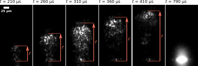
Besides the plume front propagation detected by means of the thermal radiation scattered by the bigger plume particles, a different kind of emission was typically observed on a longer timescale of the order of , as visible in the last frame of figure 5. Its continuous structure could be attributed to the ionized gas emission, which becomes visible when the plasma density reaches the camera sensitivity threshold in the region around the target surface, where locally higher temperature and density can be expected.
Figure 6 reports optical microscopy images of ablation targets for each processing condition. Different oxidation effects can be observed on the target surface. Slower pulse repetition rates corresponded to longer interactions with laser radiation and plasma, hence to larger affected zones. Almost superficial machining was obtained for the considered process parameters and materials. Therefore, target deformation could be neglected, and the SMI probe interaction can be mainly ascribed to the refraction index variations induced by the ablation plume.

IV.2 Plume front and optical path difference
An example of experimental data series is reported in figure 7 for a titanium sample with ablation pulse repetition rate equal to . The raw SMI voltage is reported in figure 7(a). The analysis algorithm identified the interferometric fringes and unwrapped the voltage fringe jumps, normalizing their amplitude to to obtain the optical path difference .
The evolution of and with time can be compared on the same timescale of figure 7(b) for the considered example. In general, after a delay of the order of – relatively to the trigger signal for the ablation laser emission, the formation of a plume front was observed with a subsequent propagation from the target surface. Simultaneously, a negative optical path difference was detected, whose absolute magnitude increased until the multi-pulse ablation was interrupted, typically reaching a maximum between and . Then, after the laser emission finished, decreased returning close to in few . This is in accordance with the model proposed for the optical path difference in the case of a ionized ablation plume, as predicted by equation (14).
The and curves within the laser emission interval were fitted to a power law to measure the dynamical scaling parameters of equations (6) and (14), and , and , respectively. A time offset parameter was included to take into account the variable delay in the laser source emission relatively to the trigger in , whose characterization was reported in figure 4. The effect of the laser emission transient was clearly visible as a delayed curve, and as a smoothing in the initial ablation stage.
Figure 8 reports another example of data series acquired for the ablation of a stainless steel specimen with . In particular, figure 8(b) represents the magnification of an example interval of , highlighting the presence of small amplitude impulses whose periodicity matches the pulse repetition rate . It can be seen that there is a good qualitative agreement with the simulated behavior reported in figure 2, which was calculated using the scaling parameters and fitting the experimental curve. This confirms the model interpretation in terms of plume accumulation. In fact, each ablation pulse generates a small contribution which tends to vanish due to its dilution within the expanding plume volume, but which gives an overall increasing trend for since the process is sustained by a series of multiple laser pulses. Finally, these observations demonstrated that SMI is in principle applicable also for the dynamical study of plumes induced by single laser pulses; however high-speed and low-noise electronics should be developed to acquire small photodiode signal variations on fast -timescales, which cannot be easily distinguished with the current setup on a limited dynamical range.
IV.3 Dynamical scaling parameters
An initial analysis was performed on the dynamical scaling exponents and , measured by fitting power laws to the and experimental curves, respectively. The results are reported in figure 9, averaging the replicates taken for each process condition and excluding experimental failures. A clear trend of and with the pulse frequency was not observed in the considered interval of . Moreover, all the exponent data points overlap each other within their uncertainties, hence differences between the considered materials are not evident from the measurements.
From a different point of view, equation (16) links the plume front exponent with the SMI optical path exponent . Therefore, it is possible to compare the experimental value of with the corresponding value derived from the model as . The results are reported in figure 10. It can be seen that the experimental points overlap within the respective error bars with the diagonal line predicted by the model, thus the observed discrepancies can be ascribable to statistical dispersion relative to a common value determined only by the expansion mechanism.
The previous observations suggest that and do not depend on target material and pulse repetition rate, as assumed in the model. Accordingly, the scaling exponents of all experiments can be reasonably averaged, finding the values reported in table 4. The average dimensionality corresponding to the plume front exponent can calculated using equation (16) as
| (18) |
which has a good correspondence with the dimensionality calculated from the optical path exponent as
| (19) |
The agreement between the two dimensionality measurements supports the validity of the model hypothesis. Moreover the results indicate that the effective plume dynamics is determined by an intermediate behavior between the planar and cylindrical expansion regimes.
| titanium | ||||
|---|---|---|---|---|
| stainless steel | ||||
| average | – |
Due to the variability observed for the scaling exponents, that strongly influences the power-law fit output, the procedure has been repeated by fixing the dimensionality to in agreement with the average experimental value . This allowed for a quantitatively consistent comparison between the different experimental conditions for the and scaling constants, and , respectively. The results are reported in figure 11. The general trend for the plume front expansion shows that the scaling constant grows with , with a faster propagation observed for titanium. Also the optical path difference scaling constant increases with the pulse repetition rate, with a faster increase for stainless steel.
IV.4 Electron number density
The average electronic density has been calculated as a function of time using equation (17), taking the plume front and SMI mean scaling constants and for the different experimental conditions. The results are reported in figure 12, with the curves being plotted on the common pulse number scale, and considering the dimensionality fixed to . The behavior found for shows that the electronic density increases rapidly after the ablation start, and it tends to saturate between and after few hundreds of laser pulses. Higher electronic densities are observed for higher pulse frequencies, with a slightly faster increase observed for stainless steel compared to titanium.

V Discussion
The experimental data presented in figure 9 suggest that the scaling exponents do not depend on the considered experimental conditions. This in accordance with the proposed model, where and depend only on the expansion dimensionality . Moreover, these exponents are linked by equation (16), which agrees with the experimental results as it was highlighted in figure 10. This provides a proof for the model validity in terms of only dynamical considerations, independently on possible absolute calibration errors or offsets.
The sign of confirms that the interferometric beam is mainly interacting with the plasma free electrons. In fact, a negative optical path difference can indicate a reduction in either the geometrical length or the refractive index. However, the former case can be excluded since the ablation processing is essentially superficial, and since returns close to after few . On the other hand, a negative refraction index variation can be the effect of a gas pressure drop, as it happens behind the shock wave front, or of the presence of free electrons. The latter is typically dominant in the case of a plasma, with the refraction index of an electron gas being smaller than the vacuum value of .
A clear difference between materials is present in the results for the scaling constants and reported in figure 11. First of all, is higher for titanium. This means that the corresponding plume expansion is faster: according to equation (6) this may be explicable in terms of a higher shock wave energy , as a consequence of a larger laser pulse energy transfer. On the contrary, is lower for titanium: this can reflect the difference observed for , as it can be derived from equations (15) and (12). Indeed, the slower plume expansion observed for stainless steel as smaller values can lead to a higher plume density in a reduced volume, hence to a higher optical path difference. However, other aspects which have not been considered in the current discussion may also influence the scaling constant results, such as the atomic ionizability or other physical properties of the materials.
The presented model links the measurement from an axial interferometric probe with the average electronic density of the expanding plume. This is particularly interesting for the potential application of the SMI technique in laser technologies involving plasma formation. As a matter of fact, equation (17) allows to calculate the mean electronic density as a function of time from the optical path difference , once the plume front scaling parameters and are known. The behavior of calculated from experimental results and reported in figure 12 is consistent with expectations. In fact, the electronic density increases with time as a consequence of accumulation during a time-distributed ionization process sustained by the ablation pulse train, with a saturation effect which resembles an equilibrium with the simultaneous plume expansion. The maximum values found for lay between and . Similar values have been observed by means of different techniques in other works related to laser ablation colombo_self-mixing_2017; pangovski_holographic_2016; zeng_experimental_2005; mao_simulation_2000.
The plume accumulation phenomenon was recently observed also by an independent theoretical study ranjbar_plume_2020. In the numerical simulations, performed in conditions similar to the ones considered here, the authors showed that in multi-pulse ablation a single shock wave arises from the pulse train, as the consequence of merging effects for the shock waves induced by the single pulses. These observations are complementary to the results presented in the current analytical and experimental study. This confirms the interpretation for plume accumulation presented here, whose preliminary quantitative characterization was reported for the first time in our previous work donadello_probing_2018: the physical properties of the ablation plume are essentially determined by the superimposition of the multiple laser pulses. Moreover the results for the numerical simulations support the interpretation for the independence of the plume dynamics on the process parameters. Indeed, the convergence to a single shock wave is reached rapidly after few pulses, therefore the presence of the subsequent pulses generates accumulation and particle mixing within the same rarefied volume, measured by , but does not alter significantly the expansion dynamics, measured by .
Quantitative considerations regarding the results for should be taken carefully. Indeed, the proposed methodology might be improved by overcoming some of the assumptions which are still present in the model. First of all, plasma lifetime should be taken into account. In fact, ionized gases undergo fast recombination at standard pressures, with the electronic density decaying on scales ranging from verhoff_dynamics_2012; zhang_investigation_2009; choudhury_time_2016; harilal_ambient_2006. Conversely a long-living plasma was assumed in the calculations. This may explain the differences between simulated and experimental optical paths in figures 2 and 8, where the experimental curve undergoes a faster decay after the laser emission end. As a matter of fact, repetitive laser pulses can strongly increase the plasma lifetime within the locally rarefied plume volume, due to self-absorption and re-heating processes as it has been observed elsewhere sangines_two-color_2011; narayanan_increasing_2007; colao_comparison_2002. Instead, after the pulse train finishes, the standard plasma lifetime determines the faster decay within the vanishing plume. Also the increase with the pulse repetition rate could be explainable in terms of such plasma lifetime enhancement. A model revision including the effects of the actual plasma lifetime might provide a more comprehensive tool for the study of plasma dynamics in ablation plumes.
The refractive index model assumed as dominant the electronic contribution, neglecting the terms related to neutral atoms and heavy ions in equation (3). Though for sufficiently ionized gases these contributes are typically negligible ascoli-bartoli_wavelength_1960; breitling_shadowgraphic_1999; ostrovskaya_holographic_2008; amer_laser-ablation-induced_2009, a second order correction might be required to accurately take into account the other plume species, which may cause a underestimation since they give opposite sign contributions to . This, in combination with the previous considerations regarding the scaling constants and , could explain the differences between materials, with being slightly higher for stainless steel compared to titanium. A possible approach that can be proposed for future studies to distinguish the refractive index contributes from the different plume species would be the implementation of a two-wavelength self-mixing interferometer. Indeed, the usage of multiple probes at different wavelengths would allow to discriminate between the plume components depending on their physical properties and their kind of dependence on ostrovskaya_holographic_2008.
A further aspect which should require a dedicated treatment is related to the expansion dimensionality , whose average value has been measured between and . Due to the axial symmetry of the problem, a mainly planar propagation can be realistically assumed. The excess related to the theoretical value of can be interpreted as the effect of a secondary and slower transverse expansion. Moreover it must be noted that the Sedov–Taylor theory for the shock wave propagation might require modifications in the case of multi-pulse laser ablation. In fact, such distributed process cannot be approximated as a single instantaneous explosion: the initial front propagation could be perturbed by the sequence of multiple pulses, deviating from the predicted power law. Therefore the resulting plume front scaling parameters and represent effective values, whose dependence on the shock wave energy and dimensionality introduced in equation (6) can be partially influenced by other parameters related to the multi-pulse laser ablation process. This may explain the effective wave energy increase which has been observed with pulse repetition rate in terms of a faster energy transfer, hence of bigger values. Such mechanism may also affect the expansion dimensionality on longer timescales. Conversely, and have been extrapolated from the initial front expansion interval which could be acquired using the high-speed camera, hypothesizing a constant propagation mechanism. Quantitative discussions should take into account of such side effects since, together with the explicit dependence on the pulse frequency in equation (15), the behavior observed for increasing with may partially explain the analogous trend of , thus of the electron number density.
VI Conclusion
In the current work, a method for evaluating the electron number density in a laser-induced plasma has been presented. A time-dependent analytical model describes the optical path difference in terms of refractive index variations, induced by plume formation during multi-pulse laser ablation. The model takes into account plasma accumulation and expansion given by such distributed process, describing the temporal evolution of the resulting electronic density as a power-law scaling.
The proposed method could be effectively applied to the SMI technique. Indeed, a coaxial SMI probe beam has been used in combination with a high-power pulsed laser to study the interaction with the plume generated at different pulse frequencies for titanium and stainless steel targets. A synchronous high-speed camera was used to observe the plume expansion and to calibrate the dynamical scaling parameters. The results for the scaling exponents are in agreement with the model predictions, with an average symmetry dimensionality measured as . The electron number density was estimated from the SMI optical path difference, showing a saturation behavior between and after few hundreds of pulses, when the plasma accumulation effect tends to balance the plume propagation.
Due to the robustness and low intrusiveness of its single-arm configuration, the results showed that SMI represents a powerful and simple tool for the dynamical study of laser-induced plumes. In fact, this method could overcome the typical measurement complexity introduced by the fast evolution of such physical systems, which are of interest in many scientific fields. Moreover, SMI can be easily integrated into industrial processes which require highly time-resolved monitoring and real-time control of gas concentration. These can include laser micromachining or pulsed laser deposition, but its application might be extended to other kinds of technologies, such as ion-beam sputtering or combustion systems, where the plasma quantification is particularly important for the process optimization.
Acknowledgments
The authors acknowledge the BLM Group for providing the acquisition setup hardware in the frame of the Project: “LT4.0” granted by the Regional Law 6/99 of the Autonomous Province of Trento, Italy. The Italian Ministry of Education, University and Research is acknowledged for the support provided through the Project “Department of Excellence LIS4.0 – Lightweight and Smart Structures for Industry 4.0”.
References
- (1) Chichkov B N, Momma C, Nolte S, von Alvensleben F and Tünnermann A 1996 Applied Physics A 63 109–115
- (2) Shirk M D and Molian P A 1998 Journal of Laser Applications 10 18–28
- (3) Amoruso S, Bruzzese R, Spinelli N and Velotta R 1999 Journal of Physics B: Atomic, Molecular and Optical Physics 32 R131
- (4) Harilal S S, Bindhu C V, Tillack M S, Najmabadi F and Gaeris A C 2003 Journal of Applied Physics 93 2380–2388
- (5) Fan C H, Sun J and Longtin J P 2002 Journal of Heat Transfer 124 275–283
- (6) Bulgakova N M, Panchenko A N, Zhukov V P, Kudryashov S I, Pereira A, Marine W, Mocek T and Bulgakov A V 2014 Micromachines 5 1344–1372
- (7) Krishnaswamy J, Rengan A, Narayan J, Vedam K and McHargue C J 1989 Applied Physics Letters 54 2455–2457
- (8) Hermann J, Thomann A L, Boulmer-Leborgne C, Dubreuil B, De Giorgi M L, Perrone A, Luches A and Mihailescu I N 1995 Journal of Applied Physics 77 2928–2936
- (9) Kwok H S, Kim H S, Kim D H, Shen W P, Sun X W and Xiao R F 1997 Applied Surface Science 109-110 595–600
- (10) Thomas J, Joshi H C, Kumar A and Philip R 2019 Journal of Physics D: Applied Physics 52 135201
- (11) Mao X, Chan W T, Caetano M, Shannon M A and Russo R E 1996 Applied Surface Science 96-98 126–130
- (12) Marla D, Bhandarkar U V and Joshi S S 2014 Applied Physics A 116 273–285
- (13) Cristoforetti G, Lorenzetti G, Benedetti P A, Tognoni E, Legnaioli S and Palleschi V 2009 Journal of Physics D: Applied Physics 42 225207
- (14) Farrokhi H, Gruzdev V, Zheng H and Zhou W 2019 Journal of the Optical Society of America B 36 1091–1100
- (15) Shaheen M E, Gagnon J E and Fryer B J 2015 Laser Physics Letters 12 066103
- (16) Singh K, Khare A and Sharma A 2017 Laser and Particle Beams 35 352–361
- (17) Stafe M, Negutu C and Popescu I M 2007 Applied Surface Science 253 6353–6358
- (18) Wen S B, Mao X, Greif R and Russo R E 2007 Journal of Applied Physics 101 023115
- (19) Farid N, Harilal S S, Ding H and Hassanein A 2014 Journal of Applied Physics 115 033107
- (20) Amoruso S, Bruzzese R, Pagano C and Wang X 2007 Applied Physics A 89 1017–1024
- (21) Tao Y, Tillack M S, Harilal S S, Sequoia K L, O’Shay B and Najmabadi F 2006 Journal of Physics D: Applied Physics 39 4027–4030
- (22) Harilal S S, Skrodzki P J, Miloshevsky A, Brumfield B E, Phillips M C and Miloshevsky G 2017 Physics of Plasmas 24 063304
- (23) Porneala C and Willis D A 2009 Journal of Physics D: Applied Physics 42 155503
- (24) Russo R, Mao X, Liu H, Yoo J and Mao S 1999 Applied Physics A 69 S887–S894
- (25) Callies G, Berger P and Hugel H 1995 Journal of Physics D: Applied Physics 28 794–806
- (26) Miyabe M, Oba M, Iimura H, Akaoka K, Khumaeni A, Kato M and Wakaida I 2015 Spectrochimica Acta Part B: Atomic Spectroscopy 110 101–117
- (27) Lednev V N, Sdvizhenskii P A, Asyutin R D, Grishin M Y, Tretyakov R S and Pershin S M 2019 Applied Optics 58 1496–1501
- (28) Verhoff B, Harilal S S, Freeman J R, Diwakar P K and Hassanein A 2012 Journal of Applied Physics 112 093303
- (29) Corsi M, Cristoforetti G, Hidalgo M, Iriarte D, Legnaioli S, Palleschi V, Salvetti A and Tognoni E 2005 Applied Spectroscopy 59 853–860
- (30) Claeyssens F, Ashfold M N R, Sofoulakis E, Ristoscu C G, Anglos D and Fotakis C 2002 Journal of Applied Physics 91 6162–6172
- (31) Choudhury K, Singh R K, Narayan S, Srivastava A and Kumar A 2016 Physics of Plasmas 23 042108
- (32) Hough P, Kelly T J, Fallon C, McLoughlin C, Hayden P, Kennedy E T, Mosnier J P, Harilal S S and Costello J T 2012 Measurement Science and Technology 23 125204
- (33) Sanginés R and Sobral H 2011 Journal of Applied Physics 110 033301
- (34) Amer E, Gren P and Sjödahl M 2008 Journal of Physics D: Applied Physics 41 215502
- (35) Pangovski K, Sparkes M and O’Neill W 2016 Advanced Optical Technologies 5 177–186
- (36) Taimre T, Nikolić M, Bertling K, Lim Y L, Bosch T and Rakić A D 2015 Advances in Optics and Photonics 7 570–631
- (37) Donati S and Norgia M 2018 Optical Engineering 57 051506
- (38) Giuliani G, Norgia M, Donati S and Bosch T 2002 Journal of Optics A: Pure and Applied Optics 4 S283–S294
- (39) Li J, Niu H and Niu Y X 2017 Optical Engineering 56 050901
- (40) Zabit U, Bernal O D and Bosch T 2013 IEEE Sensors Journal 13 824–831
- (41) Magnani A and Norgia M 2013 IEEE Journal of Quantum Electronics 49 765–769
- (42) Magnani A, Pesatori A and Norgia M 2012 Applied Optics 51 5318–5325
- (43) Donati S 2012 Laser & Photonics Reviews 6 393–417
- (44) Mezzapesa F P, Ancona A, Sibillano T, De Lucia F, Dabbicco M, Mario Lugarà P and Scamarcio G 2011 Optics Letters 36 822
- (45) Mezzapesa F P, Sibillano T, Di Niso F, Ancona A, Lugarà P M, Dabbicco M and Scamarcio G 2012 Optics Express 20 663
- (46) Demir A G, Colombo P, Norgia M and Previtali B 2016 IEEE Transactions on Instrumentation and Measurement 65 2621–2630
- (47) Colombo P, Demir A G, Norgia M and Previtali B 2017 Optics and Lasers in Engineering 92 17–28
- (48) Donadello S, Demir A G and Previtali B 2018 Evolution of laser ablation plume measured by self-mixing interferometry 2018 IEEE 4th International Forum on Research and Technology for Society and Industry (RTSI 2018) (Palermo, Italy: IEEE)
- (49) Donadello S, Demir A G and Previtali B 2018 Applied Optics 57 7232–7241
- (50) Amer E, Gren P, Kaplan A, Sjödahl M and El Shaer M 2010 Applied Surface Science 256 4633–4641
- (51) Harilal S S, Miloshevsky G V, Diwakar P K, LaHaye N L and Hassanein A 2012 Physics of Plasmas 19 083504
- (52) Mayi Y A, Dal M, Peyre P, Bellet M, Metton C, Moriconi C and Fabbro R 2019 Journal of Physics D: Applied Physics 53 075306
- (53) Ranjbar O A, Lin Z and Volkov A N 2020 Journal of Applied Physics 127 223105
- (54) Donati S, Giuliani G and Merlo S 1995 IEEE Journal of Quantum Electronics 31 113–119
- (55) Ascoli-Bartoli U, De Angelis A and Martellucci S 1960 Il Nuovo Cimento 18 1116–1137
- (56) Anders A 1990 A Formulary for Plasma Physics (Andre Anders) ISBN 978-3-05-501263-1
- (57) Ostrovskaya G V 2008 Technical Physics 53 1103
- (58) Walkup R E, Jasinski J M and Dreyfus R W 1986 Applied Physics Letters 48 1690–1692
- (59) Breitling D, Schittenhelm H, Berger P, Dausinger F and Hügel H 1999 Applied Physics A 69 S505–S508
- (60) Zhang H, Lu J, Shen Z and Ni X 2009 Optics Communications 282 1720–1723
- (61) Salimi Meidanshahi F, Madanipour K and Shokri B 2013 Optics and Lasers in Engineering 51 382–387
- (62) Amer E, Gren P and Sjödahl M 2009 Optics and Lasers in Engineering 47 793–799
- (63) Zeng X, Mao X, Greif R and Russo R 2005 Applied Physics A 80 237–241
- (64) Gupta A, Braren B, Casey K G, Hussey B W and Kelly R 1991 Applied Physics Letters 59 1302–1304
- (65) Bai W, Diebold G J, Wynn C M, Haupt R W and Doherty J H 2016 Journal of Applied Physics 120 194903
- (66) Campanella B, Legnaioli S, Pagnotta S, Poggialini F and Palleschi V 2019 Atoms 7 57
- (67) König J, Nolte S and Tünnermann A 2005 Optics Express 13 10597–10607
- (68) Zeng X, Mao X, Wen S B, Greif R and Russo R E 2004 Journal of Physics D: Applied Physics 37 1132
- (69) Demir A G, Pangovski K, O’Neill W and Previtali B 2015 Journal of Physics D: Applied Physics 48 235202
- (70) Jeong S H, Greif R and Russo R E 1998 Applied Surface Science 127-129 1029–1034
- (71) Yavas O, Maddocks E L, Papantonakis M R and Haglund R F 1998 Applied Surface Science 127-129 26–32
- (72) Jeong S H, Greif R and Russo R E 1998 Applied Surface Science 127-129 177–183
- (73) Pangovski K, Sparkes M, Cockburn A, O’Neill W, Teh P S, Lin D and Richardson D 2014 IEEE Journal of Selected Topics in Quantum Electronics 20 51–63
- (74) Breitling D, Ruf A and Dausinger F 2004 Fundamental aspects in machining of metals with short and ultrashort laser pulses Proceedings SPIE 5339 vol 5339 (International Society for Optics and Photonics) pp 49–64
- (75) Kraft S, Schille J, Mauersberger S, Schneider L and Loeschner U 2020 Applied Optics 59 452–458
- (76) Pangovski K, O’Neill W, Teh P S, Alam S, Richardson D and Demir A G 2012 Designer pulses for precise machining of silicon - A step towards photonic compositions International Congress on Applications of Lasers & Electro-Optics (Anaheim, California, USA: Laser Institute of America) pp 999–1008
- (77) Yoo J H, Jeong S H, Mao X L, Greif R and Russo R E 2000 Applied Physics Letters 76 783–785
- (78) Mao S S, Mao X, Greif R and Russo R E 2000 Applied Physics Letters 76 3370–3372
- (79) Harilal S S, O’Shay B, Tao Y and Tillack M S 2006 Journal of Applied Physics 99 083303
- (80) Narayanan V, Singh V, Pandey P K, Shukla N and Thareja R K 2007 Journal of Applied Physics 101 073301
- (81) Colao F, Lazic V, Fantoni R and Pershin S 2002 Spectrochimica Acta Part B: Atomic Spectroscopy 57 1167–1179