Bayesian Variable Selection for Cox Regression Model with Spatially Varying Coefficients with Applications to Louisiana Respiratory Cancer Data
Abstract
The Cox regression model is a commonly used model in survival analysis. In public health studies, clinical data are often collected from medical service providers of different locations. There are large geographical variations in the covariate effects on survival rates from particular diseases. In this paper, we focus on the variable selection issue for the Cox regression model with spatially varying coefficients. We propose a Bayesian hierarchical model which incorporates a horseshoe prior for sparsity and a point mass mixture prior to determine whether a regression coefficient is spatially varying. An efficient two-stage computational method is used for posterior inference and variable selection. It essentially applies the existing method for maximizing the partial likelihood for the Cox model by site independently first, and then applying an MCMC algorithm for variable selection based on results of the first stage. Extensive simulation studies are carried out to examine the empirical performance of the proposed method. Finally, we apply the proposed methodology to analyzing a real data set on respiratory cancer in Louisiana from the SEER program.
Keywords: Horseshoe Prior, Spatial Survival, SEER Data, MCMC
1 Introduction
In survival analysis, most studies focus on the overall effects of the covariates regardless of the spatial variation. In these models, associations between covariates and health outcomes are assumed to be constant. However, the effects of some covariates, such as pollution, education, employment status, may vary across different locations. Thus, models allowing for spatially varying covariate effects can be more flexible and more powerful to detect the relationship between covariates and health outcomes. From Tobler’s first law of geography (Tobler, 1970), “Everything is related to everything else, but near things are more related than distant things,” we know that the effects of covariates may be more similar to those in nearby regions than to those from distant regions due to similar environmental circumstances. Most existing literature (Banerjee and Dey, 2005; Zhou et al., 2008; Zhou et al., 2015; Zhang et al., 2016) focus on adding spatial random effects as a separate spatial component to survival models. Gelfand et al., 2003 proposed a spatially varying coefficient model which incorporates the spatial random effects by assuming the regression coefficients follow a spatial process. Reich et al., 2010 extended Gelfand’s work in the generalized linear model framework with a spike-and-slab prior. Recently, Hu and Huffer, 2020 proposed modified versions of the Kaplan–Meier and Nelson–Aalen estimators which can represent the local survival curve and cumulative hazard. Xue et al., 2020 proposed a geographically weighted Cox regression model to analyze geographically distributed survival data. But they mainly added the geographical weights to each observation without assuming any probability model on spatially varying coefficients. Hu et al., 2020 proposed a parametric accelerated failure time (AFT) model with spatially varying coefficients. Geng and Hu, 2021 explored spatial heterogeneity patterns of baseline hazards and regression coefficients. However their work was mainly concerned about the coefficient estimation and density estimation for survival models. Motivated by these works, we propose a Bayesian approach for variable selection for the Cox regression model (Cox, 1972) with spatially varying coefficients. Essentially, we add spatial correlation structure and variable selection formulation to the above mentioned spatially varying coefficient model (Gelfand et al., 2003).
In the Bayesian framework, many studies already proposed Bayesian variable selection methods for Cox models without spatially varying coefficients. Ibrahim et al., 1999 developed a semi-automatic Bayesian variable selection method for up to 20 covariates and Lee et al., 2011 built a penalized semiparametric method for high dimensional survival data. In spatial statistics, some Bayesian variable selection approaches are also well-developed. Reich et al., 2010 proposed an approach for variable selection in multivariate spatially varying coefficient regression and applied a stochastic search algorithm to determine the probabilities that each covariate’s effect is null, non-null but stationary across space, or spatially varying. Choi and Lawson, 2018 developed a flexible spatial variable selection method based on the Kuo-Mallick Entry Parameter (KMEP) method by Kuo and Mallick, 1998. In recent years, horseshoe prior (Carvalho et al., 2009; Carvalho et al., 2010) gained much attention as a shrinkage-based variable selection method because it was shown to be robust to unknown sparsity patterns and to large outlying signals. The authors also suggest it as a good default prior. We believe it can be used widely because of its robust performance. We also incorporate this prior in our proposed model.
Our model is essentially a hierarchical Bayesian model with 3 levels: The first level is a Cox proportional hazards model (Cox, 1972) with site specific spatially varying coefficients. The second level is built on each component of the regression coefficients across all sites. Here, we extend the horseshoe prior in Carvalho et al., 2009; Carvalho et al., 2010 by adding a spatial correlation matrix for variable selection. The third level is the prior belief on the hyperparameters in the second level. On estimation, we first employ the usual techniques for Cox models to maximize the partial likelihood independently for each site using R survival package. Then we model the obtained regression coefficients for each component using a multivariate normal distribution. Following the same settings in levels 2 and 3 of the original hierarchical model, we develop an MCMC algorithm for variable selection. We conduct simulation studies to illustrate our method and further apply our method to the Louisiana respiratory cancer data, which is downloaded from the Surveillance, Epidemiology, and End Results (SEER) Program.
The major contribution of this paper is to combine the horseshoe prior and spatial correlation matrix to propose a “two-stage” variable selection method for the Cox regression model with spatially varying coefficients. Horseshoe prior, which is known to be effective in handling sparsity, is a shrinkage-based variable selection prior where the selection can be achieved by setting a threshold for the local shrinkage parameter. Moreover, we add a spatial correlation matrix to the horseshoe prior and use a point mass mixture prior to further distinguish the spatially varying coefficients from spatially static coefficients. In the famous BYM model (Besag et al., 1991), the authors defined the precision matrix for the spatial random effect by the adjacency matrix and a diagonal matrix. The horseshoe prior can be applied to the precision matrix. However, we adopt the idea in Reich et al., 2010 and use the distance matrix to define the spatial correlation (covariance) matrix, which can be spatially more informative. The second contribution of this paper is on the estimation method. Instead of running an MCMC sampler based on the original model, we first estimate the Cox model for each site independently and then use the estimates from the partial likelihood to carry out an MCMC algorithm. This method is more efficient in computation than the one based on the original model.
The rest of the paper is organized as follows. In Section 2, we discuss preliminary work for spatial varying models and variable selection models. In Section 3, we introduce the proposed model with its hierarchical structure. Section 4 shows the two-stage computing method and the choice of hyperprior. We conduct three simulation studies with various degree of sparsity and spatial signal in Section 5 and illustrate our proposed method by a real data analysis on a SEER cancer study in Section 6. Some discussions about our method are presented in Section 7.
2 Preliminary Work
We first discuss some preliminary work on spatially varying coefficient models, Bayesian variable selection and graph distance that are needed for our approach.
2.1 Spatially Varying Coefficients Model
Let be a response function evaluated at the site . We can write the usual Gaussian stationary spatial process model as in, for example, Cressie, 1993,
| (1) |
where is the location mean effect, is a white noise process, and is a second-order stationary mean 0 process independent of the white noise process. To be specific, we assume , , and , where is a valid two-dimensional correlation function. Here can be treated as spatial random effects.
For linear models, (1) can be written as a spatially varying coefficient model (Gelfand et al., 2003) as following:
| (2) |
where is the covariate matrix at site and is assumed to follow a -variate spatial process model.
2.2 Bayesian Variable Selection with Shrinkage Prior
We first discuss a general Bayesian variable selection method ignoring the site effect. Let denote a -dimensional coefficients (. An easy way to incorporate sparsity in a Bayesian regression problem is to use a point mass mixture prior for each component:
| (3) |
where , and is a continuous density. And we can put a beta prior on to construct a Beta-Bernoulli prior on the model. There are a lot of computational issues due to the discontinuity of point mass mixture priors. Instead, many authors introduced continuous shrinkage priors which can be generally represented as global-local mixtures of Gaussian distributions:
| (4) |
where controls the global shrinkage and controls the local shrinkage only on . The global-local shrinkage priors have computational advantages over other variable selection priors, because the normal priors allow for conjugate updating of and , although the global-local shrinkage priors do not allow ’s to be exactly zero. There are many types of Bayesian shrinkage priors including Bayesian lasso (Park and Casella, 2008), relevance vector machine (Tipping, 2003), normal-gamma mixtures (Griffin et al., 2010) and the horseshoe prior (Carvalho et al., 2009; Carvalho et al., 2010). In horseshoe prior, in (4) is set as a standard half-Cauchy distribution , and usually is also a standard half-Cauchy distribution. For unknown sparsity patterns and large outlying signals, the horseshoe prior gives more robust results. We will apply (4) in the form of the horseshoe prior for variable selection in this paper.
2.3 Graph Distance
In this paper, we choose the graph distance as the distance measure, similar to that in Xue et al., 2020. We can define a graph by its nodes and connected with edges . Then the graph distance between two nodes and can be defined as:
| (5) |
where is the number of edges in the path. We can regard the spatial structure of Louisiana state as a graph with every county as a vertex, and there is an edge between two counties if they are adjacent. In this way, the graph distance can be calculated for every two counties using (5).
3 Bayesian Variable Selection for Cox Regression Model with Spatially Varying Coefficients
In this paper, we extend the spatially varying coefficient idea to the Cox regression model (Cox, 1972). Let be the survival time of a subject in the site and denote its hazard function for the subject with covariate vector . Then we consider the Cox model for the subject in each site ,
| (6) |
where is the hazard function with the baseline hazard , and are the -dimensional regression coefficients. For different sites, the regression model can be different since the regression coefficients are allowed to vary spatially. Assuming no ties are present among the survival times for each site. Let denote the ordered survival times from the site with being the covariate vector associated with the individual who dies at time , and denote the set of all individuals at risk prior to at site . Then the partial likelihood function for the site is written as
| (7) |
So we can maximize each partial likelihood function per site using existing software, and the corresponding estimator is called the partial maximum likelihood estimator (PMLE).
Like the usual regression models, not all the predictors have significant effects on hazards or survival times, so it would be worthwhile to develop a variable selection method for the above model. Furthermore, for the covariates selected in the model, their effects may differ among locations. Therefore, finding out which variables are spatially varying can make (6) more accurate and more flexible.
For the spatially varying coefficients model, we need to carry out variable selection in two different levels. For the first level, we need to select the variables over the whole space. That means we need to determine which variables are significant for all the locations. The second level is to determine which variables have spatially varying effects. For the significant variable selection in the first level, we extend the horseshoe prior by including a spatial correlation matrix for spatially varying coefficient models. Suppose there are sites, . Then the horseshoe version of (4) can be extended to a multidimensional horseshoe prior as:
| (8) |
where is the -th regression coefficient vector across all sites, , and is the corresponding spatial correlation matrix. controls the global variance for all the regression coefficients, and is the local variance parameter for the -th regression coefficient vector.
Note a -by- matrix, models the spatial variation of . We define the -th entry of by
| (9) |
where is the graph distance (5) between site and site . In this way, the correlation of and depends on the distance between these two sites, and for a fixed , the correlation gets smaller if two sites are more distant. The multidimensional horseshoe prior can deal with the multidimensional variable selection problems, especially when the regression coefficients are spatially dependent. In order to determine which coefficients are spatially varying over the space, we give the point mass mixture prior on as follows:
| (10) |
where is the point with mass 1 at 0, and and are the shape and rate parameters of the gamma distribution with mean . If , for any , and then ’s are perfectly positive correlated across sites. In this case, is regarded as spatially static since it doesn’t depend on the distance . If , then , so and are correlated but can vary as the distance changes. Thus, is considered to be spatially varying.
Combining (6), (8), (9) and (10), we can have the following hierarchical Bayesian variable selection model for subject in site , and .
| (11) |
In the posterior inference, a regression coefficient is regarded as not significant if the posterior mean of the corresponding local shrinkage parameter is less than 1 according to Carvalho et al., 2009; Carvalho et al., 2010. For spatially varying coefficient detection, if occurs with the posterior probability greater than , the corresponding regression coefficient is considered to be not spatially varying. Otherwise, it will be regarded as spatially varying.
4 Bayesian Computation
4.1 Two-Stage Estimation Method
In Bayesian framework, the lack of conjugacy makes it challenging to draw posterior samples for the regression coefficients in the Cox models. Considering the model complexity, we modify the “two-stage approximation” method proposed by Boehm Vock et al., 2015 to estimate the spatially varying coefficients. In the first stage, we obtain the PMLE for every site separately by maximizing the corresponding partial likelihood (7). Then the original partial likelihood can be approximated by a normal likelihood using Taylor expansion and the Fisher information matrix:
| (12) |
where are PMLEs obtained from the data at location , and is their estimated covariance matrix which summarizes the variation of the data propagated to the regression coefficients.
In the second stage, we set up a hierarchical structure on the ’s in (12) instead of the ’s in the original survival model. In this way, the ’s are regarded as the data sampled from multivariate normal distributions, and the ’s are the mean vectors of these multivariate normal distributions where the covariance matrices are known and they are basically the estimated covariance matrices of the PMLEs. Then (11) can be rewritten as:
| (13) |
where is the -th regression coefficient vector as before.
In the two-stage estimation method, the partial likelihood functions are approximated by normal likelihoods, so we only need to maximize the partial likelihood once in the first stage. Then we can build an MCMC algorithm based on (13) and such an algorithm is much more computationally efficient than that based on the original hierarchical model (11).
Note the error propagated using the two stage estimation procedure is not the same as the original hierarchical model given a is introduced. However, as the sample size in each site becomes large, we expect our two-stage procedure to work well, because the here can be thought of as the same as the in the Cox model. A reviewer suggested two different approaches for a finite sample size. One is to propagate uncertainty using multiple simulations of the results of stage 1 (Blangiardo et al., 2016; Liu et al., 2017). The other is to propagate uncertainty considering the result of stage 1 as a random variable in stage 2 with an informative prior obtained from the fit of stage 1 (Warren et al., 2012; Lee et al., 2017).
The corresponding computing method and MCMC algorithm are implemented via R package nimble (de Valpine et al., 2017). The nimble code is listed in the appendix.
4.2 Choice of Hyperprior
In practice, we find it is challenging to specify the hyperprior . It may inflate the false discovery rate if the mean of is small while the variance is relatively large, and it will inflate false omission rate if the mean is large while the variance is small. Therefore, it is appropriate to choose a gamma distribution with a moderate mean value and relatively small variance. In this paper, we choose and and it seems work well in practice regarding the balance of sensitivity and specificity . Thus, (10) can be rewritten as
| (14) |
In order to show the impacts of the hyperprior on the results, we also explore other hyperpriors in the simulation studies. Those hyperpriors include , , and . Compared to , and have the same mean but relatively large and small variances respectively, and and have the same variance but relatively small and large mean values respectively.
5 Simulation Study
We conducted three simulation studies to illustrate the two-stage variable selection method. In all simulated data sets, we consider , the number of sites and generate each predictor from a standard normal distribution. In the first simulation study, we set the first ten components of ’s to be zero vectors, that is, , so the first ten predictors are not expected to be selected in the model. The next five components , are set as spatially stationary, and they are equal to , respectively. The last five components are spatially varying coefficients and the corresponding vectors ’s are simulated from a multivariate normal distribution. For this multivariate normal distribution, each marginal is and the correlation structure is based on the geographical information of Louisiana counties. For example, the -th entry of the correlation matrix is , where is the graph distance between the -th county and the -th county. The sample size of each county is set to be 100. For each site, survival times are generated based on a Cox model with a constant baseline hazard function to be 0.5 and censored at a fixed time (155 in our example). The average censoring rate is around 35%.
The above simulation process was repeated for 100 times, and in each simulation replicate, we apply the two stage estimation method. The MCMC chain in the second stage ran for 1,000,000 iterations with the first 900,000 as burn-in. The thinning factor was 20 to improve the independence of the posterior samples. The final posterior Monte Carlo sample size was 5,000 and the variable selection capability of our model is measured using true positive rate (TPR), true negative rate (TNR), positive predictive value (PPV) and negative predictive value (NPV). The formulas are listed as follows:
Both variable selection procedures are evaluated by the above four criteria. For significant variable selection, all of the 20 predictors are considered. In this case, TP is the number of the significant predictors selected in the model while TN is the number of predictors with no effects excluded from the model. FP and FN are the number of predictors with no effects but selected into the model and the number of significant predictors that are not selected into the model, respectively. Here, we must have TP+FN=TN+FP=. In the detection of spatially varying predictors, only the last 10 predictors are under consideration since it is meaningless to find a non-significant regression coefficient to be spatially varying. TP and TN are the number of spatially varying predictors that are being regarded as spatially varying correctly and the number of spatially stationary predictors that are not being regarded as spatially varying, respectively; while FP and FN are the number of spatially stationary predictors that are regarded as spatially varying and the number of spatially varying predictors that are not being detected correctly. In this evaluation, TP+FN=TN+FP=.
Table 1 displays the simulation results discussed so far. The middle column displays the average operating characteristics for detecting a significant covariate, while the right column presents the average operating characteristics for detecting spatially varying coefficients. Corresponding standard deviations are listed in parentheses. For different hyperpriors, Gamma(25,50) can yield a good balance between TPR and TNR. Both TPR and TNR decrease if a hyperprior with a larger variance is selected, while TPR decreases but TNR increases if a smaller variance being selected. Regarding different mean values in the hyperprior, a smaller mean value will lead to a lower TNR, and a larger mean value will lead to a lower TPR. We can see our proposed method can do well in significant variable selection. For spatially varying coefficient detection, TPR and TNR are also good and both are over 80% when Gamma(25, 50) is selected, but PPV and NPV are not able to be calculated sometimes since all significant variables are regarded as spatially varying or spatially static in some simulation replicates. These findings are supported by Table 2 as well, which reports the frequencies in 100 replications of a predictor being selected and a selected predictor being spatially varying for the Gamma(25, 50) hyperprior. to can be selected and detected correctly at both levels for most of the times except that fails to be detected as spatially varying in 44 simulation replicates.
| Operating characteristics | Hyperprior | For detecting significant predictor | For detecting spatially varying coefficient |
|---|---|---|---|
| TPR % | Gamma(25,50) | 99.0(4.14) | 82.2(21.44) |
| Gamma(2.5,5) | 99.3(2.93) | 72.8(23.36) | |
| Gamma(250,500) | 98.8(3.83) | 79.0(19.15) | |
| Gamma(16,40) | 99.6(2.43) | 83.0(19.15) | |
| Gamma(36,60) | 99.1(3.21) | 69.4(23.17) | |
| TNR % | Gamma(25,50) | 99.9(1.00) | 93.2(21.88) |
| Gamma(2.5,5) | 100(0) | 90.2(26.59) | |
| Gamma(250,500) | 100(0) | 100(0) | |
| Gamma(16,40) | 99.2(4.86) | 86.8(30.91) | |
| Gamma(36,60) | 99.9(1.00) | 98.2(12.74) | |
| PPV % | Gamma(25,50) | 99.9(0.91) | NaN(NA) |
| Gamma(2.5,5) | 100(0) | NaN(NA) | |
| Gamma(250,500) | 100(0) | 100(0) | |
| Gamma(16,40) | 99.4(3.67) | NaN(NA) | |
| Gamma(36,60) | 99.9(0.91) | NaN(NA) | |
| NPV % | Gamma(25,50) | 99.1(3.41) | NaN(NA) |
| Gamma(2.5,5) | 99.4(2.57) | NaN(NA) | |
| Gamma(250,500) | 98.9(3.34) | 84.6(12.52) | |
| Gamma(16,40) | 99.7(2.09) | NaN(NA) | |
| Gamma(36,60) | 99.2(2.83) | NaN(NA) |
| being selected | detected as spatially varying | being selected | detected as spatially varying | ||
|---|---|---|---|---|---|
| 0 | (not applicable) | 93 | 8 | ||
| 0 | (not applicable) | 98 | 5 | ||
| 0 | (not applicable) | 99 | 7 | ||
| 0 | (not applicable) | 100 | 7 | ||
| 0 | (not applicable) | 100 | 7 | ||
| 0 | (not applicable) | 100 | 56 | ||
| 1 | 1 | 100 | 91 | ||
| 0 | (not applicable) | 100 | 96 | ||
| 0 | (not applicable) | 100 | 96 | ||
| 0 | (not applicable) | 100 | 72 |
We use the average mean squared error (MSE) over all sites to evaluate the accuracy of the estimator of a regression coefficient. The MSE is first calculated for each regression coefficient by site, and then averaged across all 64 sites. The results with hyperprior Gamma(25, 50) are presented in Table 3. For the non-significant variables, the estimates of the regression coefficients are very accurate, while for the significant ones, the average MSE gets larger as the magnitude of the true value increases.
| Average MSE | Average MSE | ||
|---|---|---|---|
| 0.222 | |||
| 0.865 | |||
| 1.936 | |||
| 3.429 | |||
| 5.343 | |||
| 2.209 | |||
| 2.163 | |||
| 1.993 | |||
| 2.188 | |||
| 2.223 |
To further illustrate our proposed model, we modify the sparsity patterns and spatial patterns in simulation study 2 by setting only the 19th and 20th regression coefficients as significant and only the 20th regression coefficient as spatially varying. Here , and where is the distance matrix with -th entry as . All other . In this case, it is not worthwhile to look at the operating characteristics since there are only two significant predictors and only one of them has spatially varying effects. The frequency results are presented in Table 4. Under the very sparse pattern, the significant variables can always be selected, but some non-significant variables sometimes are also selected into the model. Once they are selected, they are almost always detected to be spatially varying. In our model, there are two types of variation; variation from individuals within each site and variation across sites. We think in this scenario only two significant predictors are not sufficient to explain all the variation so some false positives are expected.
| being selected | detected as spatially varying | being selected | detected as spatially varying | ||
| 43 | 43 | 45 | 45 | ||
| 40 | 40 | 40 | 40 | ||
| 37 | 37 | 41 | 41 | ||
| 53 | 53 | 43 | 43 | ||
| 38 | 38 | 50 | 49 | ||
| 44 | 44 | 44 | 43 | ||
| 34 | 34 | 34 | 34 | ||
| 41 | 40 | 47 | 47 | ||
| 47 | 47 | 100 | 1 | ||
| 31 | 31 | 100 | 100 |
In simulation study 3, we keep the same sparsity patterns and spatial patterns as in simulation study 1 but adjust the spatial signals. For spatially varying coefficients, the spatial correlation matrix is set as instead of , which means the spatial effects are weaker than those in the simulation study 1. Corresponding results are gathered in Table 5 and 6. In this simulation study, hyperprior Gamma(25, 50) still works well and reaches a balance between TPR and TNR, and when hyperprior Gamma(25, 50) is selected, our model works well in significant variable selection but the performance is not that robust in spatially varying coefficient detection. TPR, TNR and PPV values are good but the standard deviation of TNR is large, and NPV can not be calculated since the significant regression coefficients are all regarded as spatially varying in some simulation replicates.
| Operating characteristics | Hyperprior | For detecting significant predictor | For detecting spatially varying predictor |
|---|---|---|---|
| TPR % | Gamma(25,50) | 98.9(4.69) | 88.0(13.63) |
| Gamma(2.5,5) | 80.7(7.56) | 0(0) | |
| Gamma(250,500) | 97.9(6.40) | 81.6(15.22) | |
| Gamma(16,40) | 98.4(6.77) | 89.8(12.55) | |
| Gamma(36,60) | 99.1(4.04) | 81.0(15.41) | |
| TNR % | Gamma(25,50) | 99.7(1.71) | 84.8(32.05) |
| Gamma(2.5,5) | 100(0) | 0(0) | |
| Gamma(250,500) | 100(0) | 99.8(2.00) | |
| Gamma(16,40) | 99.4(3.12) | 74.8(39.96) | |
| Gamma(36,60) | 99.7(1.71) | 96.4(16.91) | |
| PPV % | Gamma(25,50) | 99.7(1.56) | 91.1(17.42) |
| Gamma(2.5,5) | 100(0) | NaN(NA) | |
| Gamma(250,500) | 100(0) | 99.8(2.00) | |
| Gamma(16,40) | 99.5(2.65) | 86.1(20.94) | |
| Gamma(36,60) | 99.7(1.56) | 97.9(9.33) | |
| NPV % | Gamma(25,50) | 99.1(3.64) | NaN(NA) |
| Gamma(2.5,5) | 84.2(5.31) | NaN(NA) | |
| Gamma(250,500) | 98.3(5.06) | 85.8(10.94) | |
| Gamma(16,40) | 98.7(4.70) | NaN(NA) | |
| Gamma(36,60) | 99.2(3.31) | NaN(NA) |
| being selected | detected as spatially varying | being selected | detected as spatially varying | ||
|---|---|---|---|---|---|
| 1 | 1 | 92 | 12 | ||
| 0 | (not applicable) | 99 | 15 | ||
| 0 | (not applicable) | 99 | 17 | ||
| 0 | (not applicable) | 99 | 15 | ||
| 0 | (not applicable) | 100 | 16 | ||
| 1 | 1 | 100 | 51 | ||
| 1 | 1 | 100 | 100 | ||
| 0 | (not applicable) | 100 | 89 | ||
| 0 | (not applicable) | 100 | 100 | ||
| 0 | (not applicable) | 100 | 100 |
6 Data Analysis
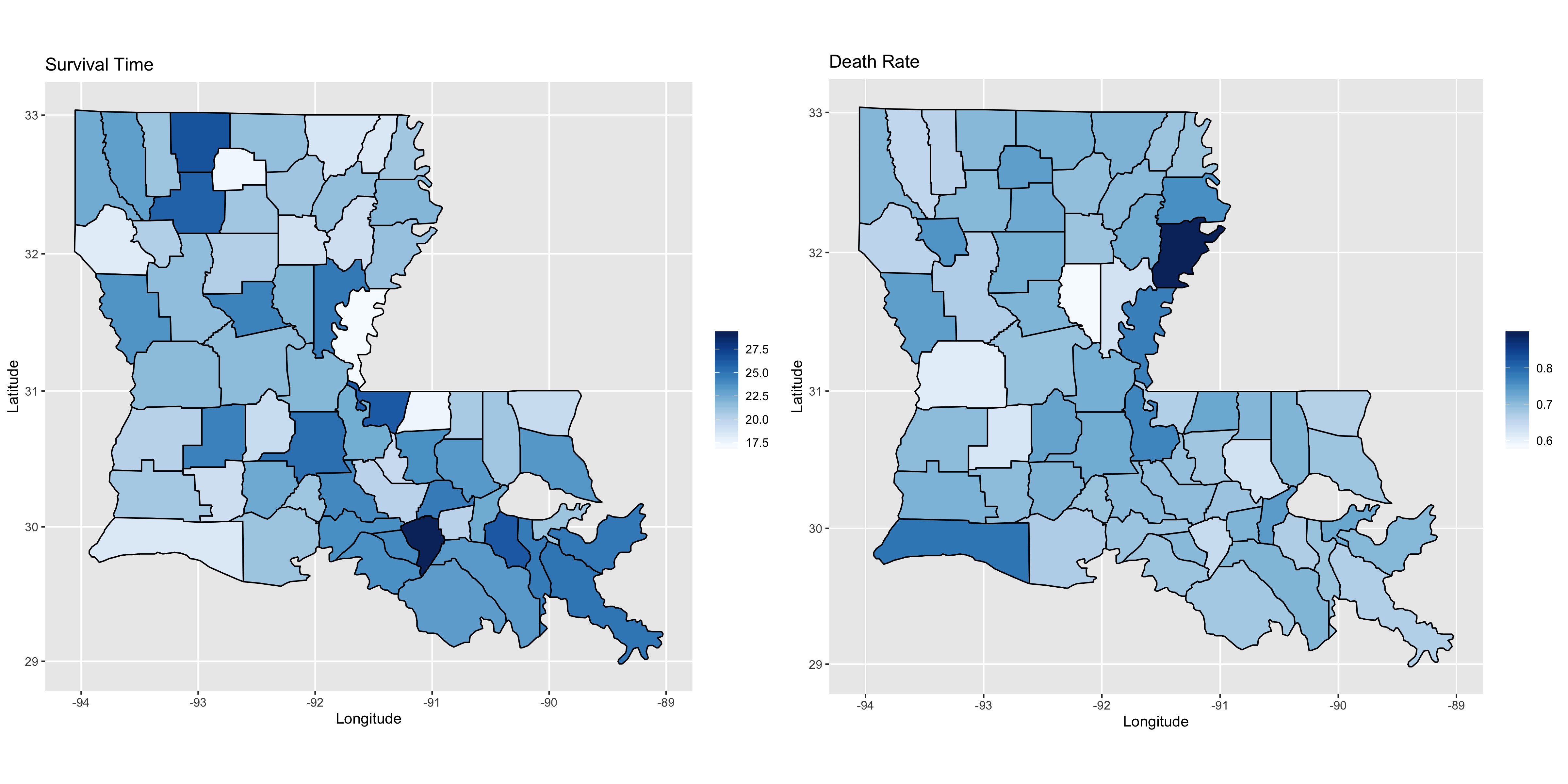
In this section, we applied our proposed method to analyzing a respiratory cancer data set in Louisiana state, which was downloaded from the Surveillance, Epidemiology, and End Results (SEER) Program (https://seer.cancer.gov/). Modifying the criteria in Zhang et al., 2016, we excluded: 1) subjects for whom the respiratory cancer was not the primary cancer; 2) subjects with unknown marital status; 3) subjects with unknown race and race other than Black and White; 4) subjects with unknown sex; 5) subjects with unknown age at diagnosis; 6) subjects with unknown cancer stage; 7) subjects with unknown cancer grade; 8) subjects with unknown surgery status; 9) subjects with unknown radiation status; 10) subjects with unknown survival times; and 11) subjects who died not because of respiratory cancer. After cleaning, there were 16213 observations left. Figure 1 displays the mean survival times and death rates for each county. It can be observed that there are large variations in mean survival times and death rates across counties.
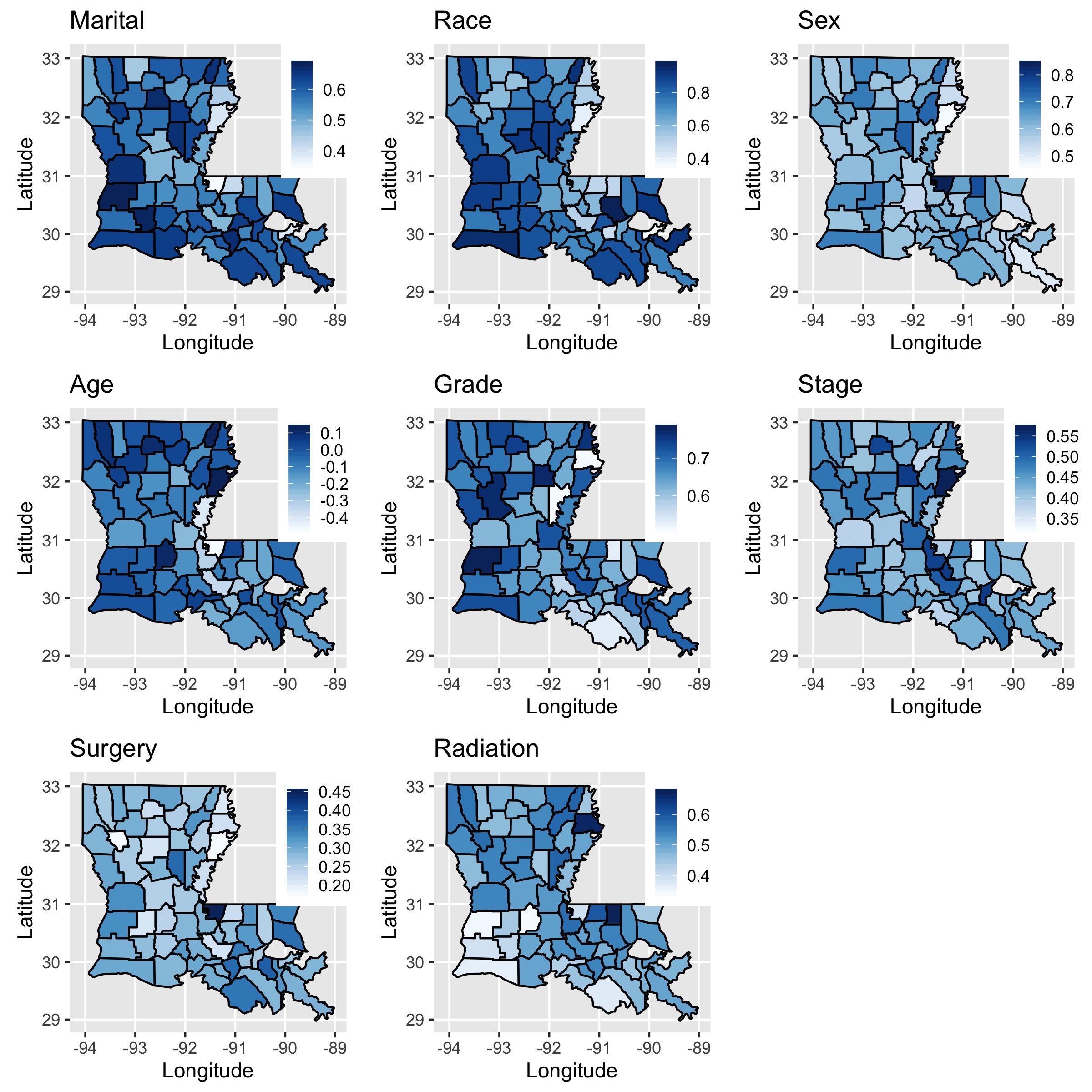
We have selected 8 variables as potential covariates from the data set. Some demographic information are available including age at diagnosis, sex (male or female) and marital status (married or not). For race, we only include the black and white since the sample sizes for other races are small. Covariate information on surgery status (yes or no) and radiation status (yes or no) are also available and thus included. As in Wu et al., 2015, we also include cancer stage and tumor grade as predictors and dichotomize them as distant or not, III or IV versus other grades, respectively. The spatial patterns of each predictor are presented in Figure 2. We can observe all the predictors have some spatial variations across different counties.
As introduced in Section 4, we first employed the Cox regression model for the data for each location. In Cameron Parish, there were only 2 white patients, resulting in inflated estimate of regression coefficient for race. Therefore, we excluded Cameron Parish from our data and 16180 observations were left. We applied our proposed model to the cleaned data set and the corresponding MCMC chain ran for 2,000,000 iterations. The burn-in number was 1,800,000 and the thinning factor was 20, so a total of 10,000 samples were used for final inference.
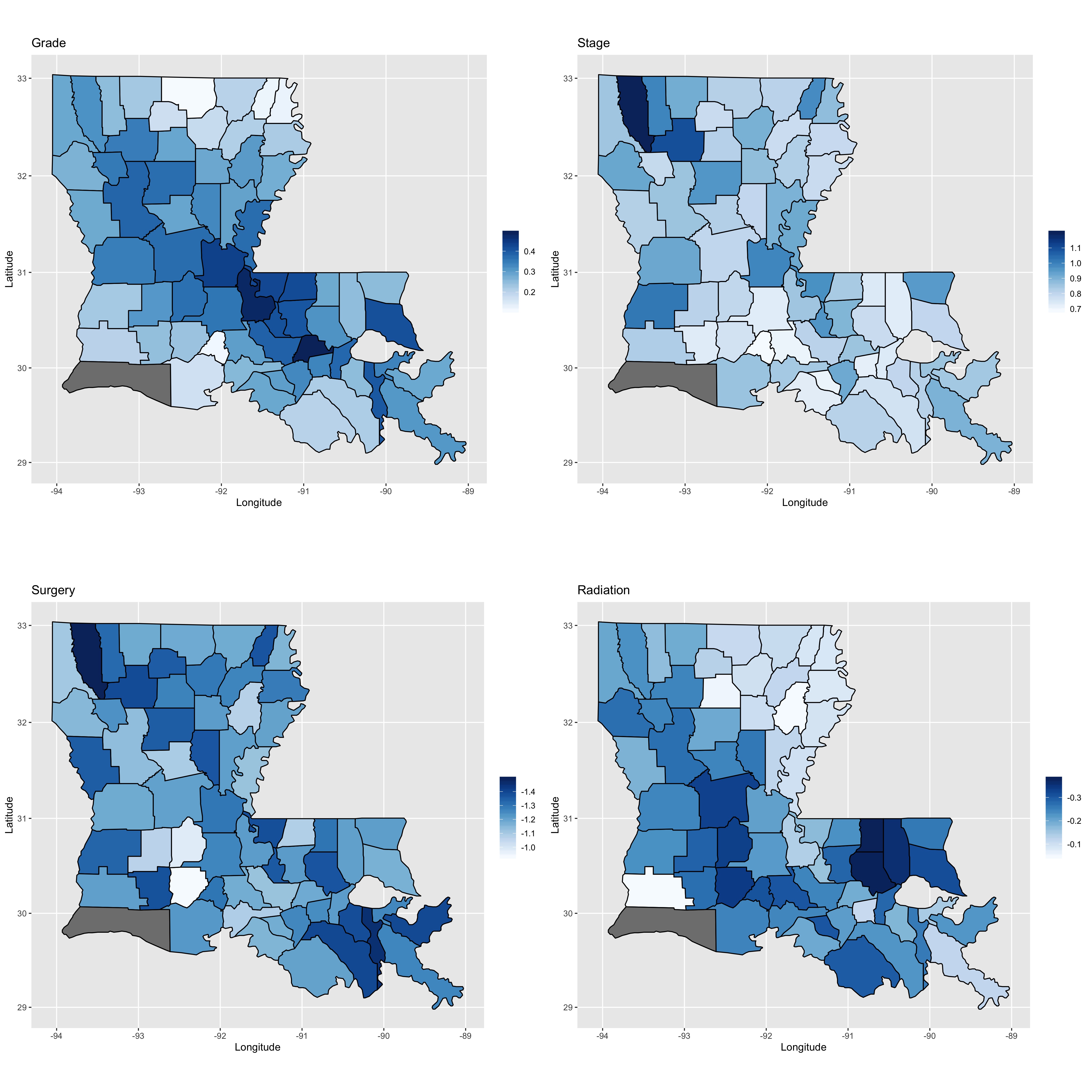
We find there are 4 variables selected into the model, including grade, stage, surgery status and radiation status, which means these four predictors have significant effects on survival times. Among these four significant predictors, grade and radiation status have spatially varying effects. Figure 3 shows the estimated values of regression coefficients of the four significant predictors. For the two spatially varying predictors, grade and radiation, we can find there are more significant spatial variation on the regression effects. Grade has larger regression effects in the central region than the surrounding areas. The low effects of radiation status mainly concentrate on a ribbon area, which is the Mississippi valley. The other two predictors, stage and surgery, were selected to be spatially stationary predictors. The results are also reasonable since the effects of stage and surgery appear to have less spatial variation, and more importantly, their variation seems spatially independent. The magnitude of the regression coefficients are randomly distributed over the whole space, instead of depending on the distance between counties.
7 Discussion
In this paper, we proposed a Bayesian variable selection method for the Cox regression model with spatially varying coefficients. We have constructed a hierarchical model for variable selection, where horseshoe priors were considered on each local smoothing and the global smoothing parameters to control sparsity. Additionally, on determining whether a coefficient is spatially varying or spatially stationary, we consider a mixture prior of a point mass and a continuous density for each entry of the spatial correlation matrix. On the computation, we have proposed a more efficient algorithm to approximate the solution. On the first stage, we derive the maximum likelihood estimates for each regression coefficient per site independently using existing software, for example, R package survival. Then we develop an MCMC algorithm for the hierarchical variable selection model based on the PMLE of the first stage. The MCMC algorithm was implemented in nimble which compiles simple R-like code into C++ for speed. The computer code is given in the Appendix.
We used three simulated data sets to illustrate our method and found that it could handle the sparsity very well when the sparsity was not that high and could also detect the spatially varying coefficients correctly in most of the situations. We have also applied our method to a real data set for respiratory cancer in Louisiana from the SEER program. Starting with eight predictors in the data set, we have selected four predictors including grade, stage, surgery status and radiation status, to be significant in the Cox regression model and two of them (grade and radiation status) were selected to be spatially varying.
The future work may involve in the improvement of the robustness of our method. As reflected from the simulation study, the performance of detecting spatially varying predictors varied a lot for different data sets. For some simulated data sets, the proposed model worked well while for some other data sets, there were some false negatives. In addition, the choice of the “slab” part of the hyperprior on can also be studied in the future since it is intricately related to the performance of the detection for spatially varying coefficients. Furthermore, the current model can only do significant variable selection overall for the whole space and then determine whether the selected variables are spatially varying. It is worthwhile to consider a site-specific selection method which allows covariates to have non-zero betas in some locations and betas=0 in other locations for the same covariates.
Appendix
In the appendix, the nimble code is listed to demonstrate the MCMC algorithm. With nimble, we can write our own code in R but in BUGS syntax and then nimble can compile our code into C++. Before building the MCMC with nimble, we first use R package survival to obtain the PMLEs and corresponding variance matrices.
Usually, a nimble model contains four parts: the model code, the constants, the data and the initial values. The first part is written with function nimbleCode and our model code is listed in the following:
The first for loop is the approximate multivariate normal distribution built on the PMLEs hatbeta and its estimated covariance matrix hatV. In the second for loop, the hierarchical structure on beta is defined as in (11) and (10). The half-Cauchy priors on global shrinkage parameter tau and local shrinkage parameter lambda[i] are given in the code below.
After defining the model, we can specify the data, the constants and the initial values as follows.
Next we can combine the four parts together using function nimbleModel and build MCMC algorithm by specifying some configurations.
In the above code, monitors refers to the parameters we mainly focus on and the corresponding posterior samples will be output. The nimble model and corresponding MCMC algorithm can be compiled into C++.
Finally, we can run our MCMC algorithm and get posterior samples. In the following code, two MCMC chains are derived, the total number of iterations is 50000 with the first 40000 as burn-in and the thinning rate is 10.
References
- Banerjee and Dey, (2005) Banerjee, S. and Dey, D. K. (2005). Semiparametric proportional odds models for spatially correlated survival data. Lifetime Data Analysis, 11(2):175–191.
- Besag et al., (1991) Besag, J., York, J., and Mollié, A. (1991). Bayesian image restoration, with two applications in spatial statistics. Annals of the Institute of Statistical Mathematics, 43(1):1–20.
- Blangiardo et al., (2016) Blangiardo, M., Finazzi, F., and Cameletti, M. (2016). Two-stage bayesian model to evaluate the effect of air pollution on chronic respiratory diseases using drug prescriptions. Spatial and Spatio-Temporal Epidemiology, 18:1–12.
- Boehm Vock et al., (2015) Boehm Vock, L. F., Reich, B. J., Fuentes, M., and Dominici, F. (2015). Spatial variable selection methods for investigating acute health effects of fine particulate matter components. Biometrics, 71(1):167–177.
- Carvalho et al., (2009) Carvalho, C. M., Polson, N. G., and Scott, J. G. (2009). Handling sparsity via the horseshoe. In International Conference on Artificial Intelligence and Statistics, volume 5, pages 73–80.
- Carvalho et al., (2010) Carvalho, C. M., Polson, N. G., and Scott, J. G. (2010). The horseshoe estimator for sparse signals. Biometrika, 97(2):465–480.
- Choi and Lawson, (2018) Choi, J. and Lawson, A. B. (2018). Bayesian spatially dependent variable selection for small area health modeling. Statistical Methods in Medical Research, 27(1):234–249.
- Cox, (1972) Cox, D. R. (1972). Regression models and life-tables. Journal of Royal Statistical Society Series B, 34:187–220.
- Cressie, (1993) Cressie, N. (1993). Statistics for Spatial Data. Wiley, New York.
- de Valpine et al., (2017) de Valpine, P., Turek, D., Paciorek, C. J., Anderson-Bergman, C., Lang, D. T., and Bodik, R. (2017). Programming with models: writing statistical algorithms for general model structures with nimble. Journal of Computational and Graphical Statistics, 26(2):403–413.
- Gelfand et al., (2003) Gelfand, A. E., Kim, H.-J., Sirmans, C., and Banerjee, S. (2003). Spatial modeling with spatially varying coefficient processes. Journal of the American Statistical Association, 98(462):387–396.
- Geng and Hu, (2021) Geng, L. and Hu, G. (2021). Bayesian spatial homogeneity pursuit for survival data with an application to the seer respiratory cancer data. Biometrics.
- Griffin et al., (2010) Griffin, J. E., Brown, P. J., et al. (2010). Inference with normal-gamma prior distributions in regression problems. Bayesian Analysis, 5(1):171–188.
- Hu and Huffer, (2020) Hu, G. and Huffer, F. (2020). Modified Kaplan–Meier estimator and Nelson–Aalen estimator with geographical weighting for survival data. Geographical Analysis, 52(1):28–48.
- Hu et al., (2020) Hu, G., Xue, Y., and Huffer, F. (2020). A Comparison of Bayesian Accelerated Failure Time Models with Spatially Varying Coefficients. Sankhyā: The Indian Journal of Statistics, Series B. Advanced online publication.
- Ibrahim et al., (1999) Ibrahim, J. G., Chen, M.-H., and MacEachern, S. N. (1999). Bayesian variable selection for proportional hazards models. Canadian Journal of Statistics, 27(4):701–717.
- Kuo and Mallick, (1998) Kuo, L. and Mallick, B. (1998). Variable selection for regression models. Sankhyā: The Indian Journal of Statistics, Series B, 60(1):65–81.
- Lee et al., (2017) Lee, D., Mukhopadhyay, S., Rushworth, A., and Sahu, S. K. (2017). A rigorous statistical framework for spatio-temporal pollution prediction and estimation of its long-term impact on health. Biostatistics, 18(2):370–385.
- Lee et al., (2011) Lee, K. H., Chakraborty, S., and Sun, J. (2011). Bayesian variable selection in semiparametric proportional hazards model for high dimensional survival data. The International Journal of Biostatistics, 7(1):1–32.
- Liu et al., (2017) Liu, Y., Shaddick, G., and Zidek, J. V. (2017). Incorporating high-dimensional exposure modelling into studies of air pollution and health. Statistics in Biosciences, 9(2):559–581.
- Park and Casella, (2008) Park, T. and Casella, G. (2008). The Bayesian Lasso. Journal of the American Statistical Association, 103(482):681–686.
- Reich et al., (2010) Reich, B. J., Fuentes, M., Herring, A. H., and Evenson, K. R. (2010). Bayesian variable selection for multivariate spatially varying coefficient regression. Biometrics, 66(3):772–782.
- Tipping, (2003) Tipping, M. (2003). Relevance vector machine. US Patent 6,633,857.
- Tobler, (1970) Tobler, W. R. (1970). A computer movie simulating urban growth in the detroit region. Economic Geography, 46(sup1):234–240.
- Warren et al., (2012) Warren, J., Fuentes, M., Herring, A., and Langlois, P. (2012). Spatial-temporal modeling of the association between air pollution exposure and preterm birth: identifying critical windows of exposure. Biometrics, 68(4):1157–1167.
- Wu et al., (2015) Wu, T. T., Li, G., and Tang, C. (2015). Empirical likelihood for censored linear regression and variable selection. Scandinavian Journal of Statistics, 42(3):798–812.
- Xue et al., (2020) Xue, Y., Schifano, E. D., and Hu, G. (2020). Geographically weighted Cox regression for prostate cancer survival data in Louisiana. Geographical Analysis, 52(4):570–587.
- Zhang et al., (2016) Zhang, Z., Sinha, S., Maiti, T., and Shipp, E. (2016). Bayesian variable selection in the AFT model with an application to the SEER breast cancer data. Statistical Methods in Medical Research.
- Zhou et al., (2015) Zhou, H., Hanson, T., Jara, A., and Zhang, J. (2015). Modelling county level breast cancer survival data using a covariate-adjusted frailty proportional hazards model. The Annals of Applied Statistics, 9(1):43.
- Zhou et al., (2008) Zhou, H., Lawson, A. B., Hebert, J. R., Slate, E. H., and Hill, E. G. (2008). Joint spatial survival modeling for the age at diagnosis and the vital outcome of prostate cancer. Statistics in Medicine, 27(18):3612–3628.