Optimal rates of convergence and error localization of Gegenbauer projections

Haiyong Wang¹¹ 1 School of Mathematics and Statistics, Huazhong University of Science and Technology, Wuhan 430074, P. R. China. E-mail: haiyongwang@hust.edu.cn ²² 2 Hubei Key Laboratory of Engineering Modeling and Scientific Computing, Huazhong University of Science and Technology, Wuhan 430074, P. R. China.

Abstract

Motivated by comparing the convergence behavior of Gegenbauer projections and best approximations, we study the optimal rate of convergence for Gegenbauer projections in the maximum norm. We show that the rate of convergence of Gegenbauer projections is the same as that of best approximations under conditions of the underlying function is either analytic on and within an ellipse and $\lambda\leq 0$ or differentiable and $\lambda\leq 1$ , where $\lambda$ is the parameter in Gegenbauer projections. If the underlying function is analytic and $\lambda>0$ or differentiable and $\lambda>1$ , then the rate of convergence of Gegenbauer projections is slower than that of best approximations by factors of $n^{\lambda}$ and $n^{\lambda-1}$ , respectively. An exceptional case is functions with endpoint singularities, for which Gegenbauer projections and best approximations converge at the same rate for all $\lambda>-1/2$ . For functions with interior or endpoint singularities, we provide a theoretical explanation for the error localization phenomenon of Gegenbauer projections and for why the accuracy of Gegenbauer projections is better than that of best approximations except in small neighborhoods of the critical points. Our analysis provides fundamentally new insight into the power of Gegenbauer approximations and related spectral methods.

Keywords: Gegenbauer projections, best approximations, analytic functions, piecewise analytic functions, functions of fractional smoothness, optimal rates of convergence

AMS classifications: 41A10, 41A25, 42C10

1 Introduction

Orthogonal polynomials are ubiquitous in approximation theory and numerical analysis and play crucial roles in numerous applications, including the construction of Gaussian quadrature (Davis & Robinowitz, 1984), the resolution of Gibbs phenomenon (Adcock & Hansen, 2012; Gelb & Tanner, 2006; Gottlieb & Shu, 1997), and spectral methods for the numerical solution of differential equations (Guo, 2000; Hesthaven et al., 2007; Olver & Townsend, 2013; Shen et al., 2011). One of the most attractive features of orthogonal polynomials is that their approximation power depends solely on the regularity of the underlying function and hence fast convergence can be achieved whenever the underlying function is sufficiently smooth. Due to the important role that orthogonal polynomials plays in diverse areas of mathematic and physics, their approximation properties have attracted considerable interest, especially in the spectral methods community (e.g., Canuto, et al., 2006; Hesthaven et al., 2007; Shen et al., 2011; Trefethen, 2013).

Let $\mathrm{d}\mu$ be a positive Borel measure on the interval $[a,b]$ , for which all moments of $\mathrm{d}\mu$ are finite. We introduce the inner product $\langle f,g\rangle_{\mathrm{d}\mu}=\int_{a}^{b}f(x)g(x)\mathrm{d}\mu(x)$ and let $\{\varphi_{k}\}_{k=0}^{\infty}$ be a set of orthogonal polynomials with respect to $\mathrm{d}\mu$ . Then, for any $f\in L^{2}([a,b])$ , it can be expanded in terms of $\{\varphi_{k}\}$ as

\displaystyle f(x)=\sum_{k=0}^{\infty}f_{k}\varphi_{k}(x),\quad f_{k}=\frac{\langle f,\varphi_{k}\rangle_{\mathrm{d}\mu}}{\langle\varphi_{k},\varphi_{k}\rangle_{\mathrm{d}\mu}}.

(1.1)

Let $S_{n}(f)$ denote the truncation of the infinite series above after the first $n+1$ terms, i.e., $S_{n}(f)=\sum_{k=0}^{n}f_{k}\varphi_{k}(x)$ , it is well known that $S_{n}(f)$ is the orthogonal projection of $f$ onto the space $\mathcal{P}_{n}=\mathrm{span}\{1,x,\ldots,x^{n}\}$ . Existing approaches for analyzing convergence of $S_{n}(f)$ in the maximum norm can be roughly categorized into two types: (i) applying the Lebesgue’s lemma $\|f-S_{n}(f)\|_{\infty}\leq(1+\Lambda)\|f-\mathcal{B}_{n}(f)\|_{\infty}$ , where $\Lambda=\sup_{f\not\equiv 0}\|S_{n}(f)\|_{\infty}/\|f\|_{\infty}$ is the Lebesgue constant of $S_{n}(f)$ and $\mathcal{B}_{n}(f)$ is the best polynomial approximation of degree $n$ to $f$ , i.e., $\|f-\mathcal{B}_{n}(f)\|_{\infty}=\min_{p\in\mathcal{P}_{n}}\|f-p\|_{\infty}$ . Hence, this approach transforms the error estimate of $S_{n}(f)$ to the problem of finding estimates for the corresponding Lebesgue constant; (ii) using the inequality $\|f-S_{n}(f)\|_{\infty}\leq\sum_{k=n+1}^{\infty}|f_{k}|\|\varphi_{k}\|_{\infty}$ , and the remaining task is to find some sharp estimates of the coefficients $\{f_{k}\}$ . The former approach plays a key role in analyzing uniform convergence of orthogonal projections and nowadays estimates for the Lebesgue constants associated with classical orthogonal projections have been well-understood. However, as far as we are aware, the sharpness of the predicted convergence rates has not been addressed. For the latter approach, a remarkable advantage is that some computable error bounds of $S_{n}(f)$ can be established (e.g., Bernstein, 1912; Liu et al., 2019; Liu et al., 2021; Trefethen, 2013; Wang & Xiang, 2012; Wang, 2018; Wang, 2021; Xiang, 2012; Xiang & Liu, 2020; Zhao et al., 2013). However, as shown in Wang (2018) and Wang (2021), the convergence rate predicted by this approach may be slower than the actual convergence rate.

In this work we are concerned with optimal rates of convergence of Gegenbauer projections in the maximum norm, i.e., $\mathrm{d}\mu(x)=(1-x^{2})^{\lambda-1/2}\mathrm{d}x$ , where $\lambda>-1/2$ and $[a,b]=[-1,1]$ . In order to exhibit the dependence on the parameter $\lambda$ , we denote by $S_{n}^{\lambda}(f)$ the Gegenbauer projection of degree $n$ . By Lebesgue’s lemma, we have

\displaystyle\|f-S_{n}^{\lambda}(f)\|_{\infty}

\displaystyle\leq(1+\Lambda_{n}(\lambda))\|f-\mathcal{B}_{n}(f)\|_{\infty},

(1.2)

where $\Lambda_{n}(\lambda)=\sup_{f\not\equiv 0}\|S_{n}^{\lambda}(f)\|_{\infty}/\|f\|_{\infty}$ is the Lebesgue constant of Gegenbauer projections. It is known from (Frenzen & Wong, 1986; Levesley & Kushpel, 1999; Lorch, 1959) that

\displaystyle\Lambda_{n}(\lambda)=\left\{\begin{array}[]{ll}{\displaystyle O(n^{\lambda})},&\hbox{$\lambda>0$,}\\[8.0pt] {\displaystyle O(\log n)},&\hbox{$\lambda=0$,}\\[8.0pt] {\displaystyle O(1)},&\hbox{$\lambda<0$.}\end{array}\right.

Note that the inequality (1.2) holds true for all $f\in{C}[-1,1]$ . One might ask how sharp the error estimates for $S_{n}^{\lambda}(f)$ obtained above are. First, it is easily seen that the predicted rate of convergence of $S_{n}^{\lambda}(f)$ is optimal in the case $\lambda<0$ since it is the same as that of $\mathcal{B}_{n}(f)$ , and is near-optimal in the case $\lambda=0$ since the Lebesgue constant $\Lambda_{n}(\lambda)$ grows very slowly as $n$ increases. In the case $\lambda>0$ , we see that the rate of convergence of $S_{n}^{\lambda}(f)$ is slower than that of $\mathcal{B}_{n}(f)$ by at most a factor of $n^{\lambda}$ . This difference may be negligible for functions which are analytic in a region containing the interval $[-1,1]$ , but will be crucial for functions which are only continuously differentiable on the interval $[-1,1]$ . More recently, the particular case of $\lambda=1/2$ , which corresponds to Legendre projections, was examined in Wang (2021). It was shown that the predicted rate of convergence by (1.2) is sharp, up to constant factors, whenever the underlying function is analytic, but is slower than the actual rate of convergence whenever the underlying function is differentiable, such as piecewise analytic functions of class $C^{s}[-1,1]$ with $s$ being a nonnegative integer (see Definition 5.1) and functions with algebraic singularities. Further, it was shown that the convergence rates of Legendre projections for these differentiable functions are actually the same as that of $\mathcal{B}_{n}(f)$ . In this perspective, it will be interesting to continue in this direction and explore the case of Gegenbauer projections.

We highlight the main contributions of this paper as follows.

(i)

If $f$ is analytic in the region bounded by the ellipse with foci $\pm 1$ and the sum of the semiminor and semimajor axes is $\rho>1$ , we improve the existing results in Wang (2016) and establish some new explicit error bounds for $S_{n}^{\lambda}(f)$ . We show that the inequality (1.2) is sharp in the sense that the convergence rate of $\mathcal{B}_{n}(f)$ is better than that of $S_{n}^{\lambda}(f)$ by a factor of $n^{\lambda}$ for $\lambda>0$ .
(ii)

If $f$ belongs to the space of piecewise analytic functions of class $C^{m-1}[-1,1]$ for some $m\in\mathbb{N}$ , we establish optimal convergence rates for $S_{n}^{\lambda}(f)$ and show that the predicted rate of convergence by the inequality (1.2) is slower than the actual rate of convergence by a factor of $n^{\min\{\lambda,1\}}$ whenever $\lambda>0$ .
(iii)

If $f$ has an interior or endpoint algebraic singularity, we carry out a convergence analysis of $S_{n}^{\lambda}(f)$ for the model function $f(x)=|x-\theta|^{\alpha}$ , where $\theta\in[-1,1]$ and $\alpha>0$ is not an even integer whenever $\theta\in(-1,1)$ and is not an integer whenever $\theta=\pm 1$ . In the case of $\theta\in(-1,1)$ , we show that the maximum error of $S_{n}^{\lambda}(f)$ is attained at one of the critical points (i.e., $x=-1,\theta,1$ ), and the predicted rate of convergence by the inequality (1.2) is slower than the actual rate of convergence by a factor of $n^{\min\{\lambda,1\}}$ for $\lambda>0$ . In the case of $\theta=\pm 1$ , we show that the maximum error of $S_{n}^{\lambda}(f)$ is attained at $x=\theta$ and the predicted rate of convergence by the inequality (1.2) in this case is slower than the actual rate of convergence by a factor of $n^{\lambda}$ for all $\lambda>0$ .
(iv)

We derive pointwise rates of convergence of $S_{n}^{\lambda}(f)$ for the model function defined above and show that the convergence rate of $S_{n}^{\lambda}(f)$ at each point $x\in(-1,\theta)\cup(\theta,1)$ is faster than that of at $x=\theta$ . As a consequence, we explain not only the error localization property of $S_{n}^{\lambda}(f)$ , i.e., the error away from the singularity is smaller than the error at the singularity, but also why the accuracy of $S_{n}^{\lambda}(f)$ is better than that of $\mathcal{B}_{n}(f)$ except in small neighborhoods of critical points.

The paper is organized as follows. In the next section, we introduce some preliminaries which will be useful in the sequel. In section 3, we carry out numerical experiments on the convergence rates of $S_{n}^{\lambda}(f)$ and $\mathcal{B}_{n}(f)$ and then give some observations. In section 4, we establish explicit error bounds of $S_{n}^{\lambda}(f)$ for analytic functions. We analyze optimal rates of convergence of $S_{n}^{\lambda}(f)$ for piecewise analytic functions of class $C^{m-1}[-1,1]$ , where $m\in\mathbb{N}$ , in section 5 and for functions with algebraic singularities in section 6. Finally, we give some concluding remarks in section 7.

2 Preliminaries

In this section, we introduce some basic properties of Gegenbauer polynomials and the gamma function that will be used throughout the paper. All these properties can be found in (Olver et al., 2010; Szegő, 1939).

2.1 Gamma function

For $\Re(z)>0$ , the gamma function is defined by

\displaystyle\Gamma(z)=\int_{0}^{\infty}t^{z-1}e^{-t}\mathrm{d}t.

(2.1)

When $\Re(z)\leq 0$ , $\Gamma(z)$ is defined by analytic continuation. The gamma function satisfies the recursive property $\Gamma(z+1)=z\Gamma(z)$ , and the classical reflection formula

\displaystyle\Gamma(z)\Gamma(1-z)=\frac{\pi}{\sin(\pi z)},\quad z\neq 0,\pm 1,\ldots.

(2.2)

Moreover, the duplication formula of the gamma function reads

\displaystyle\Gamma(2z)=\pi^{-1/2}2^{2z-1}\Gamma(z)\Gamma\left(z+\frac{1}{2}\right),\quad 2z\neq 0,-1,-2,\ldots.

(2.3)

The ratio of two gamma functions will be crucial for the derivation of explicit bounds for the Gegenbauer coefficients and the asymptotic behavior of the reproducing kernel of Gegenbauer projections. Let $a,b$ be some real or complex and bounded constants, then we have

\displaystyle\frac{\Gamma(z+a)}{\Gamma(z+b)}=z^{a-b}\left[1+\frac{(a-b)(a+b-1)}{2z}+O(z^{-2})\right],\quad z\rightarrow\infty.

(2.4)

In the special case of either $a=1$ or $b=1$ , the following sharp bounds will be useful in the subsequent analysis.

Lemma 2.1.

For $\gamma>-1$ , it holds for every $k\in\mathbb{N}$ that

\displaystyle\frac{\Gamma(k+1)}{\Gamma(k+\gamma)}\leq k^{1-\gamma}\left\{\begin{array}[]{ll}{\displaystyle\frac{1}{\Gamma(1+\gamma)}},&\hbox{$0\leq\gamma<1$,}\\[8.0pt] {\displaystyle 1},&\hbox{$-1<\gamma<0$~\text{\rm or}~$\gamma\geq 1$,}\end{array}\right.

and

\displaystyle\frac{\Gamma(k+\gamma)}{\Gamma(k+1)}\leq k^{\gamma-1}\left\{\begin{array}[]{ll}{\displaystyle 1},&\hbox{$0\leq\gamma<1$,}\\[8.0pt] {\displaystyle\Gamma(1+\gamma)},&\hbox{$-1<\gamma<0$~{\rm or}~$\gamma\geq 1$.}\end{array}\right.

Moreover, these upper bounds in (2.1) and (2.1) are sharp in the sense that they can be attained either $k=1$ or $k=\infty$ .

Proof.

We only prove (2.1) and the proof of (2.1) is completely analogous. In the cases $\gamma=0$ and $\gamma=1$ , (2.1) is trivial. Now consider the cases $-1<\gamma<0$ and $\gamma>0$ and $\gamma\neq 1$ . To this end, we introduce the following sequence

\psi(k)=\frac{\Gamma(k+1)}{\Gamma(k+\gamma)}k^{\gamma-1}.

In view of the recursive property of $\Gamma(z)$ , we obtain

\displaystyle\frac{\psi(k+1)}{\psi(k)}=\frac{k+1}{k+\gamma}\left(\frac{k+1}{k}\right)^{\gamma-1}.

By differentiating the right-hand side of the above equation with respect to $k$ , one can easily check that the sequence $\{\psi(k+1)/\psi(k)\}_{k=1}^{\infty}$ is strictly increasing whenever $0<\gamma<1$ and is strictly decreasing whenever either $-1<\gamma<0$ or $\gamma>1$ . Since $\lim_{k\rightarrow\infty}\psi(k+1)/\psi(k)=1$ , we deduce that $\{\psi(k)\}_{k=1}^{\infty}$ is strictly decreasing whenever $0<\gamma<1$ and is strictly increasing whenever either $-1<\gamma<0$ or $\gamma>1$ . Hence, for $0<\gamma<1$ , we have

\displaystyle\psi(k)\leq\psi(1)~~~\Longrightarrow~~~\frac{\Gamma(k+1)}{\Gamma(k+\gamma)}\leq\frac{k^{1-\gamma}}{\Gamma(1+\gamma)},

and the upper bound can be attained when $k=1$ . For either $-1<\gamma<0$ or $\gamma>1$ , then

\displaystyle\psi(k)\leq\lim_{k\rightarrow\infty}\psi(k)=1~~~\Longrightarrow~~~\frac{\Gamma(k+1)}{\Gamma(k+\gamma)}\leq k^{1-\gamma},

and the upper bound can be attained when $k=\infty$ . This proves (2.1) and the proof of Lemma 2.1 is complete. ∎

2.2 Gegenbauer polynomials

Let $n\geq 0$ be an integer and let $\Omega:=[-1,1]$ . The Gegenbauer polynomial of degree $n$ is defined by

\displaystyle C_{n}^{\lambda}(x)=\frac{(2\lambda)_{n}}{n!}{}_{2}\mathrm{F}_{1}\left[\begin{matrix}-n,&n+2\lambda\\ \lambda+\frac{1}{2}\hskip-28.45274pt&\end{matrix};~\frac{1-x}{2}\right],

(2.9)

where ${}_{2}\mathrm{F}_{1}(\cdot)$ is the Gauss hypergeometric function defined by

{}_{2}\mathrm{F}_{1}\left[\begin{matrix}a,~b&\\ c\end{matrix}\hskip-7.11317pt;z\right]=\sum_{k=0}^{\infty}\frac{(a)_{k}(b)_{k}}{(c)_{k}}\frac{z^{k}}{k!},

and where $(z)_{k}$ denotes the Pochhammer symbol defined by $(z)_{k}=(z)_{k-1}(z+k-1)$ for $k\in\mathbb{N}$ and $(z)_{0}=1$ . The sequence of Gegenbauer polynomials $\{C_{k}^{\lambda}(x)\}_{k=0}^{\infty}$ forms a system of polynomials orthogonal over $\Omega$ with respect to the weight function $\omega_{\lambda}(x)=(1-x^{2})^{\lambda-1/2}$ and

\int_{\Omega}\omega_{\lambda}(x)C_{m}^{\lambda}(x)C_{n}^{\lambda}(x)\mathrm{d}x=h_{n}^{\lambda}\delta_{mn},

(2.10)

where $\delta_{mn}$ is the Kronecker delta and

h_{n}^{\lambda}=\frac{\pi 2^{1-2\lambda}\Gamma(n+2\lambda)}{\Gamma(\lambda)^{2}(n+\lambda)n!},\quad\lambda>-1/2,~~\lambda\neq 0.

Since $\omega_{\lambda}(x)$ is even, it follows that $C_{n}^{\lambda}(x)$ satisfies the symmetry relation, i.e., $C_{n}^{\lambda}(x)=(-1)^{n}C_{n}^{\lambda}(-x)$ for each $n=0,1,\ldots$ , and this implies that $C_{n}^{\lambda}(x)$ is an even function for even $n$ and an odd function for odd $n$ . The Rodrigues formula of Gegenbauer polynomials reads

\displaystyle\omega_{\lambda}(x)C_{n}^{\lambda}(x)=\frac{-2\lambda}{n(n+2\lambda)}\frac{\mathrm{d}}{\mathrm{d}x}\left\{\omega_{\lambda+1}(x)C_{n-1}^{\lambda+1}(x)\right\},

(2.11)

which will be used in the asymptotic analysis of the Gegenbauer coefficients.

Next, we state some explicit bounds on the maximum value of Gegenbauer polynomials, which will be employed frequently in the convergence analysis of Gegenbauer projections.

Lemma 2.2.

If $\lambda>0$ , then for all $n\in\mathbb{N}$ ,

\displaystyle\max_{|x|\leq 1}|C_{n}^{\lambda}(x)|\leq n^{2\lambda-1}\left\{\begin{array}[]{ll}{\displaystyle\frac{1}{\Gamma(2\lambda)}},&\hbox{$0<\lambda<1/2$,}\\[10.0pt] {\displaystyle 2\lambda},&\hbox{$\lambda\geq 1/2$.}\end{array}\right.

If $-1/2<\lambda<0$ , then for all $n\in\mathbb{N}$ ,

\displaystyle\max_{|x|\leq 1}|C_{n}^{\lambda}(x)|\leq n^{\lambda-1}\left\{\begin{array}[]{ll}{\displaystyle 2^{1-\lambda}|\lambda|},&\hbox{$n=2,4,6,\ldots$,}\\[8.0pt] {\displaystyle\frac{2|\lambda|}{\sqrt{1+2\lambda}}},&\hbox{$n=1,3,5,\ldots$.}\end{array}\right.

Proof.

As for (2.2), it follows by combining the inequality $|C_{n}^{\lambda}(x)|\leq C_{n}^{\lambda}(1)=(2\lambda)_{n}/n!$ with Lemma 2.1. As for (2.2), it follows by combining equations (18.14.5) and (18.14.6) in Olver et al. (2010) with Lemma 2.1. ∎

Finally, we note that Gegenbauer polynomials include some important polynomials such as Legendre and Chebyshev polynomials as special cases, and more specifically,

\displaystyle P_{n}(x)=C_{n}^{1/2}(x),\quad U_{n}(x)=C_{n}^{1}(x),\quad n\geq 0,

(2.16)

where $P_{n}(x)$ is the Legendre polynomial of degree $n$ and $U_{n}(x)$ is the Chebyshev polynomial of the second kind of degree $n$ . When $\lambda=0$ , the Gegenbauer polynomials reduce to the Chebyshev polynomials of the first kind by the following definition

\displaystyle\lim_{\lambda\rightarrow 0^{+}}\lambda^{-1}C_{n}^{\lambda}(x)=\frac{2}{n}T_{n}(x),\quad n\geq 1,

(2.17)

where $T_{n}(x)$ is the Chebyshev polynomial of the first kind of degree $n$ .

3 Experimental observations

In this section we carry out some numerical experiments to compare the convergence behavior of $\mathcal{B}_{n}(f)$ and $S_{n}^{\lambda}(f)$ . In order to quantify the discrepancy between the rates of convergence of both methods, we introduce the quantity

\displaystyle\mathcal{R}^{\lambda}(n)=\frac{\|f-S_{n}^{\lambda}(f)\|_{\infty}}{\|f-\mathcal{B}_{n}(f)\|_{\infty}}\geq 1.

(3.1)

Moreover, using (2.10), the Gegenbauer projection $S_{n}^{\lambda}(f)$ can be written as

\displaystyle S_{n}^{\lambda}(f)

\displaystyle=\sum_{k=0}^{n}a_{k}^{\lambda}C_{k}^{\lambda}(x),\quad a_{k}^{\lambda}=\frac{1}{h_{k}^{\lambda}}\int_{\Omega}\omega_{\lambda}(x)C_{k}^{\lambda}(x)f(x)\mathrm{d}x.

(3.2)

In our computations, we compute $\mathcal{B}_{n}(f)$ using the barycentric-Remez algorithm (Pachon & Trefethen, 2009) and its implementation is available in Chebfun with the minimax command (Driscoll et al., 2014). Moreover, the maximum error of $S_{n}^{\lambda}(f)$ is measured by using a finer grid in $\Omega$ . Throughout the rest of the paper, we may use $S_{n}^{\lambda}(f,x)$ instead of $S_{n}^{\lambda}(f)$ when computing $S_{n}^{\lambda}(f)$ at the point $x$ .

Refer to caption — Figure 1: Top row shows the log plot of the maximum errors of $\mathcal{B}_{n}(f)$ ( $\bullet$ ) and $S_{n}^{\lambda}(f)$ with $\lambda=-2/5$ ( $\circ$ ) and $\lambda=-1/10$ ( $\Box$ ), for $f_{1}$ (left), $f_{2}$ (middle) and $f_{3}$ (right). Bottom row shows the plot of the corresponding $\mathcal{R}^{\lambda}(n)$ for $\lambda=-2/5$ ( $\triangleleft$ ) and $\lambda=-1/10$ ( $\triangleright$ ).

3.1 Analytic functions

We consider the following three test functions

\displaystyle f_{1}(x)=e^{2x^{3}},\quad f_{2}(x)=\ln(1.2+x),\quad f_{3}(x)=1/(1+9x^{2}).

(3.3)

We divide the choice of the parameter $\lambda$ into two ranges: $\lambda\in(-1/2,0]$ and $\lambda>0$ . Figure 1 illustrates the maximum errors of $\mathcal{B}_{n}(f)$ and $S_{n}^{\lambda}(f)$ for $\lambda=-2/5$ and $\lambda=-1/10$ and the quantity $\mathcal{R}^{\lambda}(n)$ as a function of $n$ . From the top row of Figure 1, we see that the maximum error of $\mathcal{B}_{n}(f)$ is indistinguishable with that of $S_{n}^{\lambda}(f)$ . From the bottom row of Figure 1, we see that these two $\mathcal{R}^{\lambda}(n)$ tend, respectively, to some finite constants as $n$ grows, and thus the rate of convergence of $S_{n}^{\lambda}(f)$ is the same as that of $\mathcal{B}_{n}(f)$ . Figure 2 illustrates the maximum errors of $\mathcal{B}_{n}(f)$ and $S_{n}^{\lambda}(f)$ for $\lambda=1$ and $\lambda=2$ and $n^{-\lambda}\mathcal{R}^{\lambda}(n)$ as a function of $n$ . From the top row of Figure 2, we see clearly that the rate of convergence of $\mathcal{B}_{n}(f)$ is faster than that of $S_{n}^{\lambda}(f)$ . From the bottom row of Figure 2, we see that these two $n^{-\lambda}\mathcal{R}^{\lambda}(n)$ tend, respectively, to some finite constants as $n$ grows, which imply that the rate of convergence of $S_{n}^{\lambda}(f)$ is slower than that of $\mathcal{B}_{n}(f)$ by a factor of $n^{\lambda}$ .

In summary, the above observations suggest the following conclusions:

•

For $\lambda\in(-1/2,0]$ , the rate of convergence of $S_{n}^{\lambda}(f)$ is the same as that of $\mathcal{B}_{n}(f)$ ;
•

For $\lambda>0$ , however, the rate of convergence of $S_{n}^{\lambda}(f)$ is slower than that of $\mathcal{B}_{n}(f)$ by a factor of $n^{\lambda}$ .

3.2 Differentiable functions

We consider the following test functions

\displaystyle f_{4}(x)=(x)_{+}^{4},\quad f_{5}(x)=\left|\sin(4x)\right|^{5},\quad f_{6}(x)=\left\{\begin{array}[]{ll}{\displaystyle 2\cos(x)},&\hbox{$x<0$,}\\[8.0pt] {\displaystyle 2x^{3}-x^{2}+2},&\hbox{$x\geq 0$,}\end{array}\right.

where $(x)_{+}^{k}$ is the truncated power function defined by

\displaystyle(x)_{+}^{k}=\left\{\begin{array}[]{ll}{\displaystyle x^{k}},&\hbox{$x\geq 0$,}\\[8.0pt] {\displaystyle 0},&\hbox{$x<0$,}\end{array}\right.~~k\geq 1,~~\mbox{and}~~(x)_{+}^{0}=\left\{\begin{array}[]{ll}{\displaystyle 1},&\hbox{$x\geq 0$,}\\[8.0pt] {\displaystyle 0},&\hbox{$x<0$.}\end{array}\right.

As will become clear later, the above three functions belong to the space of piecewise analytic functions of class ${C}^{m-1}(\Omega)$ with $m=4,5,3$ , respectively. In our numerical tests, we divide the choice of the parameter $\lambda$ into ranges: $\lambda\in(-1/2,1]$ and $\lambda>1$ . Figure 3 illustrates the maximum errors of $\mathcal{B}_{n}(f)$ and $S_{n}^{\lambda}(f)$ for $\lambda=-1/5$ and $\lambda=9/10$ and the quantity $\mathcal{R}^{\lambda}(n)$ as a function of $n$ . From the top row of Figure 3, we see that the maximum error of $S_{n}^{\lambda}(f)$ is slightly worse than that of $\mathcal{B}_{n}(f)$ . From the bottom row of Figure 3, we see that these two $\mathcal{R}^{\lambda}(n)$ tend to or oscillate around some finite constants as $n$ grows, which imply that the rate of convergence of $S_{n}^{\lambda}(f)$ is the same as that of $\mathcal{B}_{n}(f)$ . Figure 4 illustrates the maximum errors of $\mathcal{B}_{n}(f)$ and $S_{n}^{\lambda}(f)$ for $\lambda=3/2$ and $\lambda=3$ and $n^{1-\lambda}\mathcal{R}^{\lambda}(n)$ as a function of $n$ . From the top row of Figure 4, we see that the rate of convergence of $S_{n}^{\lambda}(f)$ is obviously slower than that of $\mathcal{B}_{n}(f)$ . From the bottom row of Figure 4, we see that these two $n^{1-\lambda}\mathcal{R}^{\lambda}(n)$ tend to or oscillate around some finite constants as $n$ grows, which imply that the rate of convergence of $S_{n}^{\lambda}(f)$ is slower than that of $\mathcal{B}_{n}(f)$ by a factor of $n^{\lambda-1}$ .

In summary, the above observations suggest the following conclusions:

•

For $\lambda\in(-1/2,1]$ , the rate of convergence of $S_{n}^{\lambda}(f)$ is the same as that of $\mathcal{B}_{n}(f)$ ;
•

For $\lambda>1$ , however, the rate of convergence of $S_{n}^{\lambda}(f)$ is slower than that of $\mathcal{B}_{n}(f)$ by a factor of $n^{\lambda-1}$ , which is one power of $n$ smaller than the predicted result using (1.2) and (1).

In the following sections, we shall carry out a convergence rate analysis of $S_{n}^{\lambda}(f)$ to explain these observations. We remark that the convergence results of the particular case $\lambda=0$ (that corresponds to Chebyshev projections) have been included in the above two observations. We refer to (Liu et al., 2019; Trefethen, 2013) for more details on the convergence rate analysis of Chebyshev projections and to Wang (2021) for a comparison of Chebyshev, Legendre projections and $\mathcal{B}_{n}(f)$ . Hereafter, we will omit discussion of this case.

4 Explicit and optimal error bounds of Gegenbauer projections for analytic functions

In this section, we establish some new error bounds of Gegenbauer projections for analytic functions. Let $\mathcal{E}_{\rho}$ denote the Bernstein ellipse

\mathcal{E}_{\rho}=\left\{z\in\mathbb{C}~\bigg|~z=\frac{u+u^{-1}}{2},~~|u|=\rho\geq 1\right\},

(4.1)

and it has foci at $\pm 1$ and the major and minor semi-axes are given by $(\rho+\rho^{-1})/2$ and $(\rho-\rho^{-1})/2$ , respectively.

The starting point of our analysis is the contour integral expression of the Gegenbauer coefficients, which was derived in Cantero & Iserles (2012) by rearranging the Taylor expansion and in Wang (2016) by rearranging the Chebyshev expansion. Here, we propose an alternative way for deriving the contour integral expression using Cauchy’s integral formula and a connection formula between the associated Legendre functions of the second kind and hypergeometric functions.

Lemma 4.1.

Suppose that $f$ is analytic in the region bounded by the ellipse $\mathcal{E}_{\rho}$ for some $\rho>1$ , then for each $k\geq 0$ and $\lambda>-1/2$ and $\lambda\neq 0$ ,

\displaystyle a_{k}^{\lambda}

\displaystyle=\frac{c_{k,\lambda}}{i\pi}\oint_{\mathcal{E}_{\rho}}\frac{f(z)}{(z\pm\sqrt{z^{2}-1})^{k+1}}{}_{2}\mathrm{F}_{1}\left[\begin{matrix}k+1,&1-\lambda\\ k+\lambda+1\hskip-28.45274pt&\end{matrix};\frac{1}{(z\pm\sqrt{z^{2}-1})^{2}}\right]\mathrm{d}z,

(4.2)

where $i$ is the imaginary unit and the sign in $z\pm\sqrt{z^{2}-1}$ is chosen so that $|z\pm\sqrt{z^{2}-1}|>1$ and

\displaystyle c_{k,\lambda}=\frac{\Gamma(\lambda)\Gamma(k+1)}{\Gamma(k+\lambda)}.

(4.3)

Proof.

By Cauchy’s integral formula and exchanging the order of integration, we obtain

	$\displaystyle a_{k}^{\lambda}$	$\displaystyle=\frac{1}{h_{k}^{\lambda}}\int_{\Omega}\omega_{\lambda}(x)C_{k}^{\lambda}(x)\left(\frac{1}{2\pi i}\oint_{\mathcal{E}_{\rho}}\frac{f(z)}{z-x}\mathrm{d}z\right)\mathrm{d}x$
		$\displaystyle=\frac{1}{\pi i}\oint_{\mathcal{E}_{\rho}}f(z)\left(\frac{1}{2h_{k}^{\lambda}}\int_{\Omega}\frac{\omega_{\lambda}(x)C_{k}^{\lambda}(x)}{z-x}\mathrm{d}x\right)\mathrm{d}z.$		(4.4)

We denote by $\Upsilon$ the term inside the bracket in the last equality. From (Gradshteyn & Ryzhik, 2007, Equation (7.312.1)) we know that $\Upsilon$ can be expressed in the form

\displaystyle\Upsilon

\displaystyle=\frac{\pi^{1/2}2^{3/2-\lambda}}{2\Gamma(\lambda)h_{k}^{\lambda}}e^{-(\lambda-1/2)\pi i}(z^{2}-1)^{\lambda/2-1/4}Q_{k+\lambda-1/2}^{\lambda-1/2}(z),

where $Q_{\nu}^{\mu}(z)$ is the associated Legendre function of the second kind of degree $\nu$ and order $\mu$ . Furthermore, using the connection formula between $Q_{\nu}^{\mu}(z)$ and ${}_{2}\mathrm{F}_{1}(\cdot)$ in (Gradshteyn & Ryzhik, 2007, Equation (8.777.2)) and the last transformation formula of ${}_{2}\mathrm{F}_{1}(\cdot)$ in (Gradshteyn & Ryzhik, 2007, Equation (9.131.1)), we have that

	$\displaystyle\Upsilon$	$\displaystyle=\frac{c_{k,\lambda}}{2^{1-2\lambda}}\frac{(z^{2}-1)^{\lambda-1/2}}{(z\pm\sqrt{z^{2}-1})^{k+2\lambda}}{}_{2}\mathrm{F}_{1}\left[\begin{matrix}k+2\lambda,&\lambda\\ k+\lambda+1\hskip-28.45274pt&\end{matrix}~;\frac{1}{(z\pm\sqrt{z^{2}-1})^{2}}\right],$
		$\displaystyle=\frac{c_{k,\lambda}}{(z\pm\sqrt{z^{2}-1})^{k+1}}{}_{2}\mathrm{F}_{1}\left[\begin{matrix}k+1,&1-\lambda\\ k+\lambda+1\hskip-28.45274pt&\end{matrix}~;\frac{1}{(z\pm\sqrt{z^{2}-1})^{2}}\right].$

Substituting this into (4) gives the desired result. This completes the proof. ∎

We now state some new bounds on the Gegenbauer coefficients $\{a_{k}^{\lambda}\}$ for all $\lambda>-1/2$ and $\lambda\neq 0$ . Compared to the previous results in Wang (2016), our bounds are new whenever $-1/2<\lambda<0$ and are more concise whenever $\lambda>0$ .

Theorem 4.2.

Under the assumptions of Lemma 4.1, we have for $\lambda\neq 0$ that

\displaystyle|a_{0}^{\lambda}|\leq D(\lambda,\rho)\left\{\begin{array}[]{ll}{\displaystyle\frac{1}{|\Gamma(\lambda)|}},&\hbox{$-1/2<\lambda<0$,}\\[12.0pt] {\displaystyle\lambda},&\hbox{$0<\lambda\leq 1$,}\\[5.0pt] {\displaystyle\frac{1}{\Gamma(\lambda)}},&\hbox{$\lambda>1$,}\end{array}\right.\quad|a_{k}^{\lambda}|

\displaystyle\leq D(\lambda,\rho)\frac{k^{1-\lambda}}{\rho^{k}},\quad k\geq 1,

where $D(\lambda,\rho)$ is defined by

\displaystyle D(\lambda,\rho)

\displaystyle=\frac{\displaystyle ML(\mathcal{E}_{\rho})}{\pi\rho}\left\{\begin{array}[]{ll}{\displaystyle\frac{\Gamma(1+\lambda)^{2}\Gamma(1-2\lambda)}{(-\lambda)\Gamma(1-\lambda)}\left(1-\frac{1}{\rho^{2}}\right)^{2\lambda-1}},&\hbox{$-1/2<\lambda<0$,}\\[15.0pt] {\displaystyle\frac{1}{\lambda}\left(1-\frac{1}{\rho^{2}}\right)^{\lambda-1}},&\hbox{$0<\lambda\leq 1$,}\\[15.0pt] {\displaystyle\Gamma(\lambda)\left(1+\frac{1}{\rho^{2}}\right)^{\lambda-1}},&\hbox{$\lambda>1$,}\end{array}\right.

and $M=\max_{z\in\mathcal{E}_{\rho}}|f(z)|$ and $L(\mathcal{E}_{\rho})$ is the length of the circumference of $\mathcal{E}_{\rho}$ .

Proof.

We follow the same line as that in Wang (2016). From Lemma 4.1 and (Wang, 2016, Theorem 4.1) we have that

\displaystyle|a_{k}^{\lambda}|

\displaystyle\leq\frac{|c_{k,\lambda}|ML(\mathcal{E}_{\rho})}{\pi\rho^{k+1}}\left\{\begin{array}[]{ll}{\displaystyle{}_{2}\mathrm{F}_{1}\left[\begin{matrix}k+1,&1-\lambda\\ k+\lambda+1\hskip-28.45274pt&\end{matrix};~\frac{1}{\rho^{2}}\right]},&\hbox{$-1/2<\lambda\leq 1$ and $\lambda\neq 0$,}\\[15.0pt] {\displaystyle{}_{2}\mathrm{F}_{1}\left[\begin{matrix}k+1,&1-\lambda\\ k+\lambda+1\hskip-28.45274pt&\end{matrix};~-\frac{1}{\rho^{2}}\right]},&\hbox{$\lambda>1$.}\end{array}\right.

It remains to bound $c_{k,\lambda}$ and these hypergeometric functions on the right-hand side of (4). For the former, it is easily seen that $|c_{k,\lambda}|=1$ when $k=0$ . For $k\geq 1$ , using Lemma 2.1 we obtain

\displaystyle|c_{k,\lambda}|\leq k^{1-\lambda}\left\{\begin{array}[]{ll}{\displaystyle|\Gamma(\lambda)|},&\hbox{$-1/2<\lambda<0$,}\\[6.0pt] {\displaystyle\lambda^{-1}},&\hbox{$0<\lambda\leq 1$,}\\[6.0pt] {\displaystyle\Gamma(\lambda)},&\hbox{$\lambda>1$.}\end{array}\right.

Next, we consider the bound of these hypergeometric functions on the right-hand side of (4). For $\lambda>0$ and $|z|<1$ , using the Euler integral representation of the Gauss hypergeometric function (Olver et al., 2010, Equation (15.6.1)), we obtain

	$\displaystyle\left\|{}_{2}\mathrm{F}_{1}\left[\begin{matrix}k+1,&1-\lambda\\ k+\lambda+1\hskip-28.45274pt&\end{matrix};~z\right]\right\|$	$\displaystyle=\frac{\Gamma(k+\lambda+1)}{\Gamma(k+1)\Gamma(\lambda)}\left\|\int_{0}^{1}t^{k}(1-t)^{\lambda-1}\left(1-zt\right)^{\lambda-1}\mathrm{d}t\right\|$
		$\displaystyle\leq\left\{\begin{array}[]{ll}{\displaystyle\left(1-\|z\|\right)^{\lambda-1}},&\hbox{$0<\lambda\leq 1$,}\\[8.0pt] {\displaystyle\left(1+\|z\|\right)^{\lambda-1}},&\hbox{$\lambda>1$.}\end{array}\right.$

For $-1/2<\lambda<0$ , it is easily verified that

\displaystyle\frac{(k+1)_{j}}{(k+\lambda+1)_{j}}\leq\frac{(1)_{j}}{(\lambda+1)_{j}},\quad\frac{(1-\lambda)_{j}}{(1+\lambda)_{j}}\leq\frac{\Gamma(1+\lambda)\Gamma(1-2\lambda)}{\Gamma(1-\lambda)}\frac{(1-2\lambda)_{j}}{(1)_{j}},

and therefore

$\displaystyle\left\|{}_{2}\mathrm{F}_{1}\left[\begin{matrix}k+1,&1-\lambda\\ k+\lambda+1\hskip-28.45274pt&\end{matrix};~z\right]\right\|$	$\displaystyle\leq\sum_{j=0}^{\infty}\frac{(k+1)_{j}(1-\lambda)_{j}}{(k+\lambda+1)_{j}}\frac{\|z\|^{j}}{j!}\leq\sum_{j=0}^{\infty}\frac{(1)_{j}(1-\lambda)_{j}}{(\lambda+1)_{j}}\frac{\|z\|^{j}}{j!}$
	$\displaystyle\leq\frac{\Gamma(1+\lambda)\Gamma(1-2\lambda)}{\Gamma(1-\lambda)}\sum_{j=0}^{\infty}\frac{(1-2\lambda)_{j}}{j!}\|z\|^{j}$
	$\displaystyle=\frac{\Gamma(1+\lambda)\Gamma(1-2\lambda)}{\Gamma(1-\lambda)}(1-\|z\|)^{2\lambda-1}.$	(4.18)

Combining (4), (4) and (4), the desired bounds follow immediately. ∎

With the above result, we are now ready to establish error bounds for Gegenbauer projections in the maximum norm, and these bounds are fully explicit with respect to the parameters $\lambda$ , $\rho$ and $n$ and are more informative than existing results. Throughout the paper, $\lfloor x\rfloor$ denotes the integer part of $x$ .

Theorem 4.3.

Suppose that $f$ is analytic in the region bounded by the ellipse $\mathcal{E}_{\rho}$ for some $\rho>1$ , and let $D(\lambda,\rho)$ be defined by (4.2).

(i)

If $\lambda>0$ , then for $n>\lfloor\eta\lambda/((\eta-1)\ln\rho)\rfloor$ and $\eta>1$ is arbitrary,

\displaystyle\|f-S_{n}^{\lambda}(f)\|_{\infty}\leq\mathcal{K}\frac{n^{\lambda}}{\rho^{n}},

(4.19)

where $\mathcal{K}$ is defined by

\displaystyle\mathcal{K}=\eta\frac{D(\lambda,\rho)}{\ln\rho}\left\{\begin{array}[]{ll}{\displaystyle\frac{1}{\Gamma(2\lambda)}},&\hbox{$0<\lambda\leq 1/2$,}\\[10.0pt] {\displaystyle 2\lambda},&\hbox{$\lambda>1/2$.}\end{array}\right.

(ii)

If $-1/2<\lambda<0$ , then for $n\geq 0$ ,

\displaystyle\|f-S_{n}^{\lambda}(f)\|_{\infty}\leq\frac{2|\lambda|D(\lambda,\rho)}{\sqrt{1+2\lambda}(\rho-1)\rho^{n}}.

(4.22)

Moreover, up to constant factors, these bounds on the right-hand side of (4.19) and (4.22) are optimal in the sense that they can not be improved in any negative powers of $n$ further.

Proof.

For part (i), combining Lemma 2.2 with Theorem 4.2 gives

\displaystyle\|f-S_{n}^{\lambda}(f)\|_{\infty}

\displaystyle\leq D(\lambda,\rho)\left(\sum_{k=n+1}^{\infty}\frac{k^{\lambda}}{\rho^{k}}\right)\left\{\begin{array}[]{ll}{\displaystyle\frac{1}{\Gamma(2\lambda)}},&\hbox{$0<\lambda\leq 1/2$,}\\[10.0pt] {\displaystyle 2\lambda},&\hbox{$\lambda>1/2$.}\end{array}\right.

For the sum inside the bracket, one can easily check that $k^{\lambda}/\rho^{k}$ is strictly decreasing with respect to $k$ whenever $k\geq\lambda/\ln\rho$ , and thus

\displaystyle\sum_{k=n+1}^{\infty}\frac{k^{\lambda}}{\rho^{k}}

\displaystyle\leq\int_{n}^{\infty}\frac{x^{\lambda}}{\rho^{x}}\mathrm{d}x=\frac{\Gamma(\lambda+1,n\ln\rho)}{(\ln\rho)^{1+\lambda}},

(4.25)

where $\Gamma(a,x)$ is the incomplete gamma function (see, e.g., Olver et al., p. 174). Furthermore, from Natalini & Palumbo (2000) we know that $|\Gamma(a,x)|\leq\eta x^{a-1}e^{-x}$ for $a>1$ and $x>(a-1)\eta/(\eta-1)$ and $\eta>1$ is arbitrary, the desired result (4.19) follows. The proof of part (ii) is similar and we omit the details.

We now turn to prove the optimality of (4.19) and (4.22). Here we only prove the former since the latter can be proved by a similar argument. Suppose by contradiction that there exist constants $\gamma,c>0$ independent of $n$ such that

\displaystyle\|f-S_{n}^{\lambda}(f)\|_{\infty}\leq c\frac{n^{\lambda-\gamma}}{\rho^{n}}.

(4.26)

We consider the function $f(x)=1/(x-\omega)$ with $\omega+\sqrt{\omega^{2}-1}>1+\lambda^{-1}$ . It is easily seen that this function has a simple pole at $x=\omega$ and therefore $\rho\leq\omega+\sqrt{\omega^{2}-1}-\epsilon$ , where $\epsilon>0$ may be taken arbitrary small. Using Lemma 4.1 and the residue theorem, we can write the Gegenbauer coefficients of $f(x)$ as

\displaystyle a_{k}^{\lambda}

\displaystyle=\frac{(-2c_{k,\lambda})}{(\omega+\sqrt{\omega^{2}-1})^{k+1}}{}_{2}\mathrm{F}_{1}\left[\begin{matrix}k+1,&1-\lambda\\ k+\lambda+1\hskip-28.45274pt&\end{matrix};~\frac{1}{(\omega+\sqrt{\omega^{2}-1})^{2}}\right].

(4.27)

Clearly, we see that $a_{k}^{\lambda}<0$ for all $k\geq 0$ . Moreover, by considering the ratio $a_{k+1}^{\lambda}/a_{k}^{\lambda}$ , it is not difficult to verify that the sequence $\{a_{k}^{\lambda}\}_{k=0}^{\infty}$ is strictly increasing. We now consider the error of $S_{n}^{\lambda}(f)$ at the point $x=1$ . Recall the well-known inequality $\max_{|x|\leq 1}|C_{k}^{\lambda}(x)|\leq C_{k}^{\lambda}(1)$ for $\lambda>0$ and $k\in\mathbb{N}$ , we obtain that

\displaystyle|f(1)-S_{n}^{\lambda}(f,1)|

\displaystyle=-\sum_{k=n+1}^{\infty}a_{k}^{\lambda}C_{k}^{\lambda}(1)\geq-a_{n+1}^{\lambda}C_{n+1}^{\lambda}(1).

Combining this with (4.26) we deduce that

\displaystyle-a_{n+1}^{\lambda}C_{n+1}^{\lambda}(1)\leq\|f(x)-S_{n}^{\lambda}(f)\|_{\infty}\leq c\frac{n^{\lambda-\gamma}}{\rho^{n}}.

(4.28)

By using (4), (2.4) and (4.27), we obtain that $|a_{n+1}^{\lambda}C_{n+1}^{\lambda}(1)|=O(n^{\lambda}(\omega+\sqrt{\omega^{2}-1})^{-n})$ . On the other hand, we know that $n^{\lambda-\gamma}\rho^{-n}=O(n^{\lambda-\gamma}(\omega+\sqrt{\omega^{2}-1}-\epsilon)^{-n})$ . This leads to a contradiction since the upper bound may be smaller than the lower bound when $\epsilon$ is sufficiently small. Therefore, we can conclude that the derived bound (4.19) is optimal and can not be improved in any negative powers of $n$ . This completes the proof. ∎

Remark 4.4.

From Cheney (1998) and Bernstein (1912) we know that $\|f-\mathcal{B}_{n}(f)\|_{\infty}=O(\rho^{-n})$ . Comparing this with (4.19) and (4.22), it is easily seen that the rate of convergence of $S_{n}^{\lambda}(f)$ is slower than that of $\mathcal{B}_{n}(f)$ by a factor of $n^{\lambda}$ for $\lambda>0$ and is the same as that of $S_{n}^{\lambda}(f)$ for $-1/2<\lambda<0$ , which fully explains the convergence behavior of $S_{n}^{\lambda}(f)$ illustrated in Figures 1 and 2.

Remark 4.5.

Polynomial interpolation in the zeros of Gegenbauer polynomials is also a powerful approach for approximating analytic functions. When the interpolation nodes are the zeros of $C_{n+1}^{\lambda}(x)$ , it has been shown in (Xie et al., 2013, Theorem 4.1) that the rate of convergence of Gegenbauer interpolation in the maximum norm is $O(n^{\lambda}\rho^{-n})$ for $\lambda>0$ and is $O(\rho^{-n})$ if $-1/2<\lambda<0$ . Comparing this with Theorem 4.3, we see that Gegenbauer interpolation and projection of the same degree possess the same convergence rate.

5 Optimal rates of convergence of Gegenbauer projections for piecewise analytic functions

In this section we study optimal rates of convergence of Gegenbauer projections for piecewise analytic functions of class $C^{m-1}(\Omega)$ with $m\in\mathbb{N}$ . Throughout this paper, we denote by $K$ a generic positive constant independent of $n$ which may take different values at different places.

We first introduce the definitions of piecewise analytic functions and the space of piecewise analytic functions of class $C^{m-1}(\Omega)$ .

Definition 5.1.

Let $m$ be a positive integer.

(i)

A function $f$ is said to be piecewise analytic on $\Omega$ if there exists a set of distinct points $\{\xi_{1},\ldots,\xi_{\ell}\}$ with each $\xi_{k}\in(-1,1)$ and $\xi_{k}<\xi_{k+1}$ for $k=1,\ldots,\ell-1$ and $\ell\in\mathbb{N}$ , such that the restriction of $f$ to each of the intervals $[-1,\xi_{1}]$ , $[\xi_{1},\xi_{2}]$ , $\ldots$ , $[\xi_{\ell},1]$ has an analytic continuation to a neighborhood of this closed interval, but $f$ itself is not analytic at each point of $\{\xi_{1},\ldots,\xi_{\ell}\}$ . Moreover, we call these points $\{\xi_{1},\ldots,\xi_{\ell}\}$ the singularities of $f$ .
(ii)

The space of piecewise analytic functions of class $C^{m-1}(\Omega)$ is defined to be the set of piecewise analytic functions on $\Omega$ satisfying $f\in C^{m-1}(\Omega)$ .

With the above definitions, it is easily verified that these test functions in (3.2) are piecewise analytic functions of class $C^{m-1}(\Omega)$ with $m=4,5,3$ , respectively. We now consider optimal convergence rates of Gegenbauer projections for piecewise analytic functions of class $C^{m-1}(\Omega)$ . First of all, using the integral expression of Gegenbauer coefficients, we can rewrite the Gegenbauer projection as

\displaystyle S_{n}^{\lambda}(f)

\displaystyle=\int_{\Omega}\omega_{\lambda}(t)f(t)D_{n}^{\lambda}(x,t)\mathrm{d}t,

(5.1)

where $D_{n}^{\lambda}(\cdot,\cdot)$ is the reproducing kernel of Gegenbauer projection defined by

	$\displaystyle D_{n}^{\lambda}(x,t)$	$\displaystyle=\sum_{k=0}^{n}\frac{C_{k}^{\lambda}(x)C_{k}^{\lambda}(t)}{h_{k}^{\lambda}}$
		$\displaystyle=\frac{\Gamma(\lambda)^{2}}{2^{2-2\lambda}\pi}\frac{\Gamma(n+2)}{\Gamma(n+2\lambda)}\frac{C_{n+1}^{\lambda}(x)C_{n}^{\lambda}(t)-C_{n+1}^{\lambda}(t)C_{n}^{\lambda}(x)}{x-t},$		(5.2)

and the last equation follows from the Christoffel-Darboux formula of Gegenbauer polynomials.

The following refined estimates for the reproducing kernel will be useful.

Lemma 5.2.

Let $|x|\leq 1$ . Then, for $\lambda\neq 0$ and large $n$ ,

(i)

If $|t|\leq 1$ , it holds that $|D_{n}^{\lambda}(x,t)|\leq Kn^{2\max\{\lambda,0\}+1}$ .
(ii)

If $|t|\leq 1-\varepsilon$ with $\varepsilon\in(0,1)$ , it holds that $|D_{n}^{\lambda}(x,t)|\leq Kn^{\max\left\{\lambda,1\right\}}$ .

Proof.

We first consider part (i). From Lemma 2.2 we see that

\displaystyle\max_{|x|\leq 1}|C_{n}^{\lambda}(x)|=\left\{\begin{array}[]{ll}{\displaystyle O(n^{2\lambda-1})},&\hbox{$\lambda>0$,}\\[8.0pt] {\displaystyle O(n^{\lambda-1})},&\hbox{$-1/2<\lambda<0$.}\end{array}\right.

Moreover, using (2.4) we have $h_{n}^{\lambda}=O(n^{2\lambda-2})$ . Combining these estimates we find that

\displaystyle|D_{n}^{\lambda}(x,t)|\leq\sum_{k=0}^{n}\frac{|C_{k}^{\lambda}(x)C_{k}^{\lambda}(t)|}{h_{k}^{\lambda}}=\sum_{k=0}^{n}O(k^{2\max\{\lambda,0\}})=O(n^{2\max\{\lambda,0\}+1}).

This proves part (i). To prove part (ii), we distinguish two cases: $|x-t|<\varepsilon/2$ and $|x-t|\geq\varepsilon/2$ . For the case $|x-t|<\varepsilon/2$ , it is easily verified that $|x|\leq 1-\varepsilon/2$ . Recall from Szegő (1939) that $|C_{n}^{\lambda}(x)|=O(n^{\lambda-1})$ for $x\in(-1,1)$ , we obtain

\displaystyle\max_{\begin{subarray}{c}|x|\leq 1-\varepsilon/2\\ |t|\leq 1-\varepsilon\end{subarray}}\frac{|C_{k}^{\lambda}(x)C_{k}^{\lambda}(t)|}{h_{k}^{\lambda}}=O(1),

and thus

\displaystyle|D_{n}^{\lambda}(x,t)|\leq\sum_{k=0}^{n}\frac{|C_{k}^{\lambda}(x)C_{k}^{\lambda}(t)|}{h_{k}^{\lambda}}=\sum_{k=0}^{n}O(1)=O(n).

Next, we consider the case $|x-t|\geq\varepsilon/2$ . Combining the estimate $\max_{|t|\leq 1-\varepsilon}|C_{n}^{\lambda}(t)|=O(n^{\lambda-1})$ with (5), and the last equality in (5), we immediately infer that

\displaystyle|D_{n}^{\lambda}(x,t)|=O(n^{\max\{\lambda,0\}}).

A combination of the above two estimates gives part (ii). This completes the proof. ∎

Now, we prove the main result of this section.

Theorem 5.3.

If $f$ belongs to the space of piecewise analytic functions of class $C^{m-1}(\Omega)$ for some $m\in\mathbb{N}$ . Then, for $\lambda<m+1$ and $n\gg 1$ ,

\displaystyle\|f-S_{n}^{\lambda}(f)\|_{\infty}\leq K\left\{\begin{array}[]{ll}{\displaystyle n^{-m}},&\hbox{$\lambda\leq 1$,}\\[8.0pt] {\displaystyle n^{-m-1+\lambda}},&\hbox{$\lambda>1$.}\end{array}\right.

Moreover, the convergence rates on the right-hand side of (5.3) are optimal in the sense that they can not be improved further.

Proof.

Assume that $\{\xi_{1},\ldots,\xi_{\ell}\}$ , with $\ell\in\mathbb{N}$ , are the singularities of $f$ . For every $\eta\in(0,1)$ , we know from Saff & Totik (1989) that there exists a polynomial $\psi_{n}$ of degree $n$ such that

\displaystyle|f(x)-\psi_{n}(x)|\leq\frac{C}{n^{m}}\exp\left(-\kappa(n\mathrm{d}(x))^{\eta}\right),\quad\forall x\in\Omega,

(5.7)

where $\mathrm{d}(x)=\min_{1\leq k\leq\ell}|x-\xi_{k}|$ and $C,\kappa$ are some positive constants. Recall that $S_{n}^{\lambda}(f)\equiv f$ whenever $f\in\mathcal{P}_{n}$ , we immediately obtain

$\displaystyle\|f(x)-S_{n}^{\lambda}(f,x)\|$	$\displaystyle=\|f(x)-\psi_{n}(x)-S_{n}^{\lambda}(f-\psi_{n},x)\|$
	$\displaystyle\leq\|f(x)-\psi_{n}(x)\|+\|S_{n}^{\lambda}(f-\psi_{n},x)\|$
	$\displaystyle\leq\frac{C}{n^{m}}\exp\left(-\kappa(n\mathrm{d}(x))^{\eta}\right)$
	$\displaystyle~~~~~~+\frac{C}{n^{m}}\int_{\Omega}\exp\left(-\kappa(n\mathrm{d}(t))^{\eta}\right)\omega_{\lambda}(t)\|D_{n}^{\lambda}(x,t)\|\mathrm{d}t.$	(5.8)

We now consider the estimate of the last integral in (5). For simplicity of notation we denote it by $I$ . Moreover, let $\Omega_{k}=[\xi_{k}-\gamma,\xi_{k}+\gamma]$ , where $k=1,\ldots,\ell$ and $\gamma>0$ is chosen such that these subintervals $\Omega_{1},\ldots,\Omega_{\ell}\subset(-1,1)$ are pairwise disjoint and thus,

	$\displaystyle I$	$\displaystyle=\sum_{k=1}^{\ell}\int_{\Omega_{k}}\exp\left(-\kappa(n\mathrm{d}(t))^{\eta}\right)\omega_{\lambda}(t)\|D_{n}^{\lambda}(x,t)\|\mathrm{d}t$
		$\displaystyle~~~~~~~~+\int_{\Omega\backslash\bigcup_{k=1}^{\ell}\Omega_{k}}\exp\left(-\kappa(n\mathrm{d}(t))^{\eta}\right)\omega_{\lambda}(t)\|D_{n}^{\lambda}(x,t)\|\mathrm{d}t.$		(5.9)

Let $I_{1}$ and $I_{2}$ denote the first and second terms on the right-hand side of (5), respectively. For $I_{1}$ , notice that $\mathrm{d}(t)=|t-\xi_{k}|$ whenever $t\in\Omega_{k}$ , and thus from Lemma 5.2 we have

$\displaystyle I_{1}$	$\displaystyle\leq\max_{t\in\bigcup_{k=1}^{\ell}\Omega_{k}}\|\omega_{\lambda}(t)\|Kn^{\max\{\lambda,1\}}\sum_{k=1}^{\ell}\int_{\Omega_{k}}\exp\left(-\kappa(n\mathrm{d}(t))^{\eta}\right)\mathrm{d}t$
	$\displaystyle=\max_{t\in\bigcup_{k=1}^{\ell}\Omega_{k}}\|\omega_{\lambda}(t)\|(2\ell K)n^{\max\{\lambda,1\}-1}\int_{0}^{n\gamma}\exp\left(-\kappa\nu^{\eta}\right)\mathrm{d}\nu$
	$\displaystyle=O(n^{\max\{\lambda,1\}-1}),$	(5.10)

where we have applied the change of variable $t=\xi_{k}+\nu/n$ in the second step. For $I_{2}$ , notice that $\mathrm{d}(t)\geq\gamma$ whenever $t\in\Omega\backslash\bigcup_{k=1}^{\ell}\Omega_{k}$ , and using Lemma 5.2 again, we obtain

$\displaystyle I_{2}$	$\displaystyle\leq\exp\left(-\kappa(n\gamma)^{\eta}\right)\int_{\Omega}\omega_{\lambda}(t)\|D_{n}^{\lambda}(x,t)\|\mathrm{d}t$
	$\displaystyle\leq\exp\left(-\kappa(n\gamma)^{\eta}\right)Kn^{2\max\{\lambda,0\}+1}\int_{\Omega}\omega_{\lambda}(t)\mathrm{d}t$
	$\displaystyle=O(\exp\left(-\kappa(n\gamma)^{\eta}\right)n^{2\max\{\lambda,0\}+1}).$	(5.11)

Combining (5), (5), (5) and (5) gives (5.3).

We now turn to prove the optimality of the convergence rates on the right-hand side of (5.3). Recall that $\|f-\mathcal{B}_{n}(f)\|_{\infty}=O(n^{-m})$ (see, e.g., Timan, 1963, Chapter 7). In the case $\lambda\leq 1$ , the rate of convergence of $S_{n}^{\lambda}(f)$ is obviously optimal since it is the same as that of $\mathcal{B}_{n}(f)$ . In the case $\lambda>1$ , the predicted convergence rate is $\|f-S_{n}^{\lambda}(f)\|_{\infty}=O(n^{-m-1+\lambda})$ . To show the optimality of this rate, we consider a specific example $f(x)=(x)_{+}^{5}$ , which corresponds to $m=5$ . In view of (Olver et al., 2010, Equation (18.17.37)), the Gegenbauer coefficients of this function are given by

\displaystyle a_{k}^{\lambda}

\displaystyle=\frac{15}{8}\frac{\Gamma(\lambda)(k+\lambda)}{\Gamma(\lambda+\frac{k+7}{2})\Gamma(\frac{7-k}{2})},\quad k=0,1,\ldots,

(5.12)

from which we can see that $a_{2k+1}^{\lambda}=0$ for $k\geq 3$ . For $k\geq 6$ is even, we have, using (2.2) and (2.4),

\displaystyle a_{k}^{\lambda}

\displaystyle=(-1)^{\frac{k}{2}+1}\frac{15\Gamma(\lambda)}{8\pi}\frac{(k+\lambda)\Gamma(\frac{k-5}{2})}{\Gamma(\frac{k+7}{2}+\lambda)}=(-1)^{\frac{k}{2}+1}\frac{15\Gamma(\lambda)}{4\pi}\left(\frac{k}{2}\right)^{-\lambda-5}+O(k^{-\lambda-6}).

(5.13)

Now we consider the error estimate of $S_{n}^{\lambda}(f)$ at $x=1$ . Assume that $n\geq 6$ is a large even integer, using (5.13) and the asymptotic estimate $C_{k}^{\lambda}(1)=k^{2\lambda-1}/\Gamma(2\lambda)+O(k^{2\lambda-2})$ , we obtain that

	$\displaystyle f(1)-S_{n}^{\lambda}(f,1)$	$\displaystyle=\sum_{k=1}^{\infty}a_{n+2k}^{\lambda}C_{n+2k}^{\lambda}(1)$
		$\displaystyle\sim(-1)^{\frac{n}{2}+1}\frac{15\Gamma(\lambda)2^{\lambda+3}}{\pi\Gamma(2\lambda)}n^{\lambda-6}\sum_{k=1}^{\infty}(-1)^{k}\left(1+\frac{2k}{n}\right)^{\lambda-6}$
		$\displaystyle=O(n^{\lambda-6}),\qquad n\gg 1,$

where in the last step we have used the fact that the alternating series is always bounded for $\lambda<6$ . Similarly, it is not difficult to show that $f(1)-S_{n}^{\lambda}(f,1)=O(n^{\lambda-6})$ if $n\geq 6$ is a large odd integer. Since $\|f-S_{n}^{\lambda}(f)\|_{\infty}\geq|f(1)-S_{n}^{\lambda}(f,1)|$ , we can conclude that the predicted rate $\|f-S_{n}^{\lambda}(f)\|_{\infty}=O(n^{\lambda-6})$ is optimal. This completes the proof. ∎

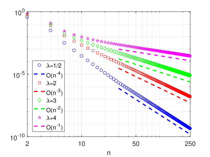
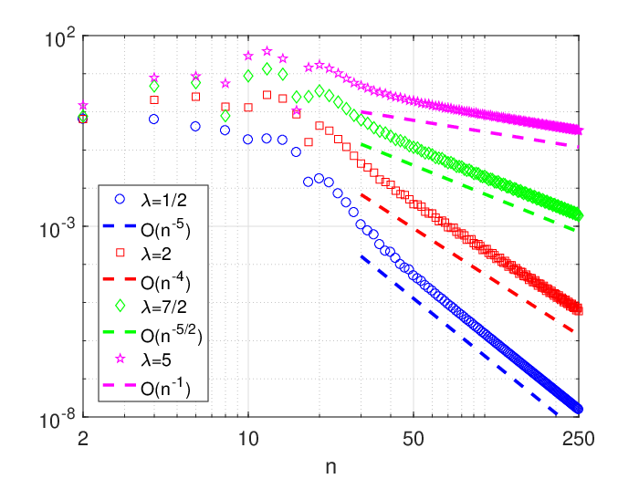
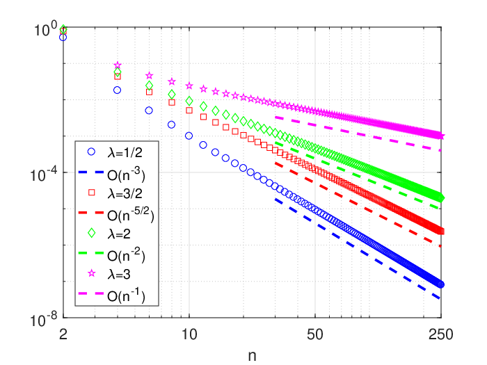
In order to verify the convergence rates predicted by Theorem 5.3, we consider the test functions in (3.2), which correspond to $m=4,5,3$ , respectively. From Theorem 5.3 we know that the predicted rate of $S_{n}^{\lambda}(f_{4})$ is $O(n^{-4})$ if $\lambda\leq 1$ and is $O(n^{\lambda-5})$ if $\lambda>1$ , and the predicted rate of $S_{n}^{\lambda}(f_{5})$ is $O(n^{-5})$ if $\lambda\leq 1$ and is $O(n^{\lambda-6})$ if $\lambda>1$ , and the predicted rate of $S_{n}^{\lambda}(f_{6})$ is $O(n^{-3})$ if $\lambda\leq 1$ and is $O(n^{\lambda-4})$ if $\lambda>1$ . For each $f_{j}$ , we test the convergence rates of $S_{n}^{\lambda}(f_{j})$ with four values of $\lambda$ and they are displayed in Figure 5. Clearly, for each $\lambda$ , we see that the actual convergence rate of $S_{n}^{\lambda}(f)$ coincides quite well with the predicted rate. Moreover, these results also explain the observations in Figures 3 and 4 since the convergence rates of $\mathcal{B}_{n}(f)$ for $f_{4},f_{5}$ and $f_{6}$ are $O(n^{-4}),O(n^{-5})$ and $O(n^{-3})$ , respectively.

6 Optimal rates of convergence of Gegenbauer projections for functions with algebraic singularities

In this section we consider optimal rates of convergence of Gegenbauer projections for functions with algebraic singularities. Specifically, we divide our discussion into two cases: (i) functions with an interior singularity; (ii) functions with an endpoint singularity. For ease of clarity and conciseness, we restrict ourselves to the following model function

\displaystyle f(x)=|x-\theta|^{\alpha},

(6.1)

where $\theta\in\Omega$ and $\alpha>0$ is not an even integer whenever $\theta\in(-1,1)$ and is not an integer whenever $\theta=\pm 1$ . The convergence rate results will shed light on the study of more complicated functions with algebraic singularities.

Remark 6.1.

Although we restrict ourselves to the model function (6.1), the extension to more general functions involving one or more singularities of $|x-\theta|^{\alpha}$ -type, such as $f(x)=\sum_{k=1}^{m}|x-\theta_{k}|^{\alpha_{k}}g_{k}(x)$ , where $-1\leq\theta_{1}<\cdots<\theta_{m}\leq 1$ and $\alpha_{k}>0$ are not integers and $g_{k}(x)$ are sufficiently smooth, is straightforward. Moreover, for functions of the form $f(x)=g(x)\prod_{k=1}^{m}|x-\theta_{k}|^{\alpha_{k}}$ , where $g(x)$ is sufficiently smooth, by noticing that they can also be decomposed into a sum of $m$ functions and each function contains exactly one singularity of $|x-\theta|^{\alpha}$ -type (Tuan & Elliott, 1972), our analysis can also be applied to handle such functions.

6.1 The case $\theta\in(-1,1)$

In the case where $\alpha$ is an odd integer, note that $f$ belongs to the space of piecewise analytic functions of class $C^{\alpha-1}(\Omega)$ , and thus the optimal rate of convergence of $S_{n}^{\lambda}(f)$ follows immediately from Theorem 5.3. In the case where $\alpha$ is not an integer, however, Theorem 5.3 can not be used and a new approach for error estimates of $S_{n}^{\lambda}(f)$ should be developed.

Before we proceed, let us consider the location of the maximum error of $S_{n}^{\lambda}(f)$ . In the particular case $\lambda=1/2$ , which corresponds to Legendre projections, it has been observed in Wang (2021) that the maximum error is attained at $x=\theta$ . For the Gegenbauer case, however, the situation may be complicated and it is highly interesting to clarify the dependence of the location of the maximum error on the parameter $\lambda$ . To gain some insight, we plot in Figure 6 the pointwise error of $S_{n}^{\lambda}(f)$ with three values of $\lambda$ . Clearly, we observe that, for $\lambda$ greater than a critical value, the location of the maximum error of $S_{n}^{\lambda}(f)$ will jump from $x=\theta$ to one of the endpoints $x=1$ or $x=-1$ . Motivated by this observation, we shall consider the pointwise error of $S_{n}^{\lambda}(f)$ and then clarify the maximum error of $S_{n}^{\lambda}(f)$ .

We start with the following result.

Lemma 6.2.

Let $f$ be defined by (6.1) with $\theta\in(-1,1)$ and let $\alpha>0$ be not an even integer.

(i)

For each $k\geq\alpha+1$ ^*^* * This condition is imposed here due to the definition of generalized Gegenbauer functions proposed in (Liu et al., 2019, Definition 2.1). However, numerical tests show that the formula ((i)) is valid for all $k\geq 0$ . To keep the proof concise, we will not pursue this here.,

	$\displaystyle a_{k}^{\lambda}$	$\displaystyle=\omega_{\lambda+\alpha+1}(\theta)\frac{\Gamma(\lambda)\Gamma(\alpha+1)(k+\lambda)}{2^{1+\alpha}\Gamma(\lambda+\alpha+\frac{3}{2})\sqrt{\pi}}\left({}_{2}\mathrm{F}_{1}\left[\begin{matrix}\alpha+1-k,&k+2\lambda+\alpha+1\\ \alpha+\lambda+\frac{3}{2}\hskip-28.45274pt&\end{matrix};~\frac{1-\theta}{2}\right]\right.$
		$\displaystyle~~~~~~~~~~\left.+~(-1)^{k}{}_{2}\mathrm{F}_{1}\left[\begin{matrix}\alpha+1-k,&k+2\lambda+\alpha+1\\ \alpha+\lambda+\frac{3}{2}\hskip-28.45274pt&\end{matrix};~\frac{1+\theta}{2}\right]\right).$		(6.2)

(ii)

As $k\rightarrow\infty$ ,

	$\displaystyle a_{k}^{\lambda}$	$\displaystyle=-\omega_{\frac{\lambda+\alpha+1}{2}}(\theta)\sin\left(\frac{\alpha\pi}{2}\right)\frac{2^{1+\lambda}\Gamma(\lambda)\Gamma(\alpha+1)}{\pi k^{\alpha+\lambda}}\cos\left(2(k+\lambda)\phi(\theta)-\frac{\lambda\pi}{2}\right)$
		$\displaystyle~~~~~+O(k^{-\alpha-\lambda-1}),$		(6.3)

where $\phi(\theta)=\arccos(\sqrt{(1+\theta)/2})$ .

The proof of Lemma 6.2 is postponed to Appendix A.

Remark 6.3.

An immediate corollary of Lemma 6.2 is the comparison of decay rates of Chebyshev and Legendre coefficients, which was studied in Boyd & Petschek (2014) and Wang (2016). More specifically, let $k\geq 1$ and let $a_{k}^{L}$ and $a_{k}^{C}$ , respectively, denote the $k$ th Legendre and Chebyshev coefficients of $f$ defined by (6.1), i.e.,

\displaystyle a_{k}^{L}=\frac{2k+1}{2}\int_{\Omega}f(x)P_{k}(x)\mathrm{d}x,\quad a_{k}^{C}=\frac{2}{\pi}\int_{\Omega}\frac{f(x)T_{k}(x)}{\sqrt{1-x^{2}}}\mathrm{d}x.

(6.4)

It has been observed in the right panel of Figure 7 in Wang (2016) that $a_{k}^{C}$ decays faster than $a_{k}^{L}$ by a factor of $O(k^{1/2})$ and the sequence $\{a_{k}^{L}/a_{k}^{C}k^{-1/2}\}$ oscillates around a finite value as $k\rightarrow\infty$ . However, a theoretical explanation for this observation is still lacking. To clarify this issue, using ((ii)) and (2.17), after some simplifications, we obtain that

\displaystyle\frac{a_{k}^{L}}{a_{k}^{C}}

\displaystyle=\omega_{\frac{3}{4}}(\theta)\frac{\cos\left((2k+1)\phi(\theta)-\frac{\pi}{4}\right)}{\cos\left(2k\phi(\theta)\right)}\left(\frac{\pi k}{2}\right)^{1/2}+O(k^{-1/2}).

(6.5)

Consequently, we can see that the sequence $\{a_{k}^{L}/a_{k}^{C}k^{-1/2}\}$ oscillates around a finite value as $k\rightarrow\infty$ whenever $\theta\neq 0$ and tends to the constant $(\pi/2)^{1/2}$ whenever $\theta=0$ .

The following lemma will also be useful.

Lemma 6.4.

Let $\nu\in\mathbb{R}$ and $\nu(\mathrm{mod}~2\pi)\neq 0$ . Then, for $\mu<0$ , it holds that

\displaystyle\chi_{\mu,\nu}(n):=\sum_{k=n}^{\infty}e^{ik\nu}k^{\mu}=O(n^{\mu}),\quad n\rightarrow\infty.

(6.6)

Proof.

For $\mu<-1$ , the desired estimate follows immediately from (Olver, 1974, Equation (5.10)). For $-1\leq\mu<0$ , using the identity (Olver, 1974, Equation (5.09)), we have that

\displaystyle\chi_{\mu,\nu}(n)=\frac{(-\mu)e^{i\nu}}{e^{i\nu}-1}\chi_{\mu-1,\nu}(n)-\frac{e^{in\nu}}{e^{i\nu}-1}n^{\mu}+O(n^{\mu-1}).

Since $\chi_{\mu-1,\nu}(n)=O(n^{\mu-1})$ in this case, the desired estimate follows immediately. ∎

The main theorem in this subsection is now given as follows.

Theorem 6.5.

Let $f$ be defined by (6.1) with $\theta\in(-1,1)$ and let $\alpha>0$ be not an even integer. Then, for $\lambda<\alpha+1$ and $n\gg 1$ , it holds that

(i)

The maximum error of $S_{n}^{\lambda}(f)$ satisfies

\displaystyle\|f-S_{n}^{\lambda}(f)\|_{\infty}=\left\{\begin{array}[]{ll}{\displaystyle O(n^{-\alpha})},&\hbox{$\lambda\leq 1$,}\\[8.0pt] {\displaystyle O(n^{-\alpha-1+\lambda})},&\hbox{$\lambda>1$.}\end{array}\right.

(ii)

For $x\in\Omega$ , the pointwise error estimate of $S_{n}^{\lambda}(f)$ is

\displaystyle|f(x)-S_{n}^{\lambda}(f,x)|=\left\{\begin{array}[]{ll}{\displaystyle O(n^{-\alpha-1+\lambda})},&\hbox{$x=\pm 1$,}\\[8.0pt] {\displaystyle O(n^{-\alpha})},&\hbox{$x=\theta$,}\\[8.0pt] {\displaystyle O(n^{-\alpha-1})},&\hbox{$x\in(-1,\theta)\cup(\theta,1)$.}\end{array}\right.

Proof.

We only consider the proof of part (ii) since part (i) is a direct consequence of part (ii). We start with the error estimate of $S_{n}^{\lambda}(f)$ at $x=1$ . From Lemma 6.2 and the fact that $C_{k}^{\lambda}(1)=k^{2\lambda-1}/\Gamma(2\lambda)+O(k^{2\lambda-2})$ , we have

	$\displaystyle f(1)-S_{n}^{\lambda}(f,1)$	$\displaystyle=-\omega_{\frac{\lambda+\alpha+1}{2}}(\theta)\sin\left(\frac{\alpha\pi}{2}\right)\frac{2^{1+\lambda}\Gamma(\lambda)\Gamma(\alpha+1)}{\pi\Gamma(2\lambda)}$
		$\displaystyle~~~~~\times\sum_{k=n+1}^{\infty}\left(\frac{\cos\left(2(k+\lambda)\phi(\theta)-\frac{\lambda\pi}{2}\right)}{k^{\alpha+1-\lambda}}+O(k^{-\alpha+\lambda-2})\right).$

Furthermore, we note that $\phi(\theta)\in(0,\pi/2)$ and

	$\displaystyle\sum_{k=n+1}^{\infty}\frac{\cos\left(2(k+\lambda)\phi(\theta)-\frac{\lambda\pi}{2}\right)}{k^{\alpha+1-\lambda}}$	$\displaystyle=\cos\left(2\lambda\phi(\theta)-\frac{\lambda\pi}{2}\right)\sum_{k=n+1}^{\infty}\frac{\cos\left(2k\phi(\theta)\right)}{k^{\alpha+1-\lambda}}$
		$\displaystyle~-\sin\left(2\lambda\phi(\theta)-\frac{\lambda\pi}{2}\right)\sum_{k=n+1}^{\infty}\frac{\sin\left(2k\phi(\theta)\right)}{k^{\alpha+1-\lambda}},$

and therefore, by Lemma 6.4, these two sums on the right-hand side behave like $O(n^{-\alpha-1+\lambda})$ . This proves the error estimate of $S_{n}^{\lambda}(f)$ at $x=1$ . The error estimate of $S_{n}^{\lambda}(f)$ at $x=-1$ can be proved in a similar way and we omit the details.

Next, we consider the error estimate of $S_{n}^{\lambda}(f)$ at $x\in(-1,1)$ . For notational simplicity, we set $x=\cos\zeta$ , where $\zeta\in(0,\pi)$ . According to Theorem 8.21.8 in Szegő (1939),

\displaystyle C_{k}^{\lambda}(x)=\frac{(1-x^{2})^{-\lambda/2}}{\Gamma(\lambda)}\left(\frac{2}{k}\right)^{1-\lambda}\cos\left((k+\lambda)\zeta-\frac{\lambda\pi}{2}\right)+O(k^{\lambda-2}).

(6.12)

Combining (6.12) with ((ii)) in Lemma 6.2, after some simplification, we arrive at

	$\displaystyle f(x)-S_{n}^{\lambda}(f,x)$	$\displaystyle=\sum_{k=n+1}^{\infty}a_{k}^{\lambda}C_{k}^{\lambda}(x)$
		$\displaystyle=-2\sin\left(\frac{\alpha\pi}{2}\right)\omega_{\frac{\lambda+\alpha+1}{2}}(\theta)\Gamma(\alpha+1)\frac{(1-x^{2})^{-\lambda/2}}{\pi}$
		$\displaystyle~~~~\times\left[\sum_{k=n+1}^{\infty}\frac{\cos\left((k+\lambda)(2\phi(\theta)-\zeta)\right)+\cos\left((k+\lambda)(2\phi(\theta)+\zeta)-\lambda\pi\right)}{k^{\alpha+1}}\right]$
		$\displaystyle~~~~+O(n^{-\alpha-1}).$

We denote with $J$ the term inside the bracket on the right-hand side of the above equation and it is easily seen that the error estimate of $S_{n}^{\lambda}(f)$ is completely determined by the asymptotic behavior of $J$ . We now consider the error estimate of $S_{n}^{\lambda}(f)$ at the singularity $x=\theta$ . In this case, it is easily checked that $\zeta=\arccos\theta=2\phi(\theta)$ , and thus

	$\displaystyle J$	$\displaystyle=\sum_{k=n+1}^{\infty}\frac{1+\cos\left((k+\lambda)(2\zeta)-\lambda\pi\right)}{k^{\alpha+1}}$
		$\displaystyle=\sum_{k=n+1}^{\infty}\frac{1}{k^{\alpha+1}}+\cos((\pi-2\zeta)\lambda)\sum_{k=n+1}^{\infty}\frac{\cos(2k\zeta)}{k^{\alpha+1}}+\sin((\pi-2\zeta)\lambda)\sum_{k=n+1}^{\infty}\frac{\sin(2k\zeta)}{k^{\alpha+1}}.$

Clearly, the first sum behaves like $O(n^{-\alpha})$ and the last two sums, in view of Lemma 6.4, behave like $O(n^{-\alpha-1})$ . Hence, we conclude that $J=O(n^{-\alpha})$ and this proves the error estimate of $S_{n}^{\lambda}(f)$ at $x=\theta$ . Finally, we consider the error estimate of $S_{n}^{\lambda}(f)$ at $x\in(-1,1)\backslash\{\theta\}$ . In this case, we note that

	$\displaystyle J$	$\displaystyle=\cos(\lambda(2\phi(\theta)-\zeta))\sum_{k=n+1}^{\infty}\frac{\cos(k(2\phi(\theta)+\zeta))}{k^{\alpha+1}}$
		$\displaystyle-\sin(\lambda(2\phi(\theta)-\zeta))\sum_{k=n+1}^{\infty}\frac{\sin(k(2\phi(\theta)+\zeta))}{k^{\alpha+1}}$
		$\displaystyle+\cos(\lambda(2\phi(\theta)+\zeta-\pi))\sum_{k=n+1}^{\infty}\frac{\cos(k(2\phi(\theta)+\zeta))}{k^{\alpha+1}}$
		$\displaystyle-\sin(\lambda(2\phi(\theta)+\zeta-\pi))\sum_{k=n+1}^{\infty}\frac{\sin(k(2\phi(\theta)+\zeta))}{k^{\alpha+1}},$

and by using Lemma 6.4 again and the fact that $2\phi(\theta)+\zeta\in(0,2\pi)$ , these four sums on the right-hand side all behave like $O(n^{-\alpha-1})$ . Therefore, we conclude that $J=O(n^{-\alpha-1})$ and this proves the error estimate of $S_{n}^{\lambda}(f)$ at $x\in(-1,1)\backslash\{\theta\}$ . This completes the proof. ∎

Several remarks on Theorem 6.5 are in order.

Remark 6.6.

Recall from Timan (1963) that the rate of convergence of $\mathcal{B}_{n}(f)$ in the maximum norm is $O(n^{-\alpha})$ . Therefore, the rate of convergence of $S_{n}^{\lambda}(f)$ is the same as that of $\mathcal{B}_{n}(f)$ whenever $-1/2<\lambda\leq 1$ . For $\lambda>1$ , however, the rate of convergence of $S_{n}^{\lambda}(f)$ is slower than that of $\mathcal{B}_{n}(f)$ by a factor of $n^{\lambda-1}$ , which is one power of $n$ better than the result predicted by (1.2).

Remark 6.7.

Pointwise error estimates of Jacobi projections were studied in Agahanov & Natanson (1966) in the space

W_{\mu}^{\nu}(\Omega)=\left\{f~\big|~f,f{{}^{\prime}},\cdots,f^{(\nu-1)}\in\mathrm{AC}(\Omega),~f^{(\nu)}\in\mathrm{H}^{\mu}(\Omega)\right\},

where $\nu\in\mathbb{N}$ , $\mu\in[0,1]$ and $\mathrm{AC}(\Omega)$ denotes the space of absolutely continuous functions and $\mathrm{H}^{\mu}(\Omega)$ denotes the space of Hölder continuous function with exponent $\mu$ . When restricting their results to the case of Gegenbauer projections and the model function (6.1), their results can be written as

|f(x)-S_{n}^{\lambda}(f,x)|=\left\{\begin{array}[]{ll}{\displaystyle O(n^{\lambda-\alpha})},&\hbox{$x=\pm 1$,}\\[8.0pt] {\displaystyle O(n^{-\alpha}\ln n)},&\hbox{$x\in(-1,1)$.}\end{array}\right.

Compared with Theorem 6.5, it is clear to see that our results are sharper.

In Figure 7 we illustrate the maximum error of $S_{n}^{\lambda}(f)$ for the test function $f(x)=|x+0.4|^{5/2}$ . As expected, the predicted convergence rates by ((i)) agree quite well with the observed convergence rates.

6.2 The case $\theta=\pm 1$

Error estimates of Gegenbauer projections for functions with endpoint singularities have been studied in the recent work Xiang & Liu (2020) and optimal convergence rates of $S_{n}^{\lambda}(f)$ in the maximum norm have been derived based on optimal decay rates of the Gegenbauer coefficients. Here we revisit this issue and provide a more thorough insight.

Theorem 6.8.

Let $f$ be defined by (6.1) with $\theta=\pm 1$ and $\alpha>0$ is not an integer.

(i)

For $\lambda>0$ and $n\geq\lfloor\alpha\rfloor$ , the maximum error of $S_{n}^{\lambda}(f)$ is attained at $x=\theta$ and

\displaystyle\|f-S_{n}^{\lambda}(f)\|_{\infty}=\frac{2^{\alpha}|\sin(\alpha\pi)|\Gamma(\alpha+\lambda+\frac{1}{2})\Gamma(\alpha)}{\pi\Gamma(\lambda+\frac{1}{2})n^{2\alpha}}+O(n^{-2\alpha-1}).

(6.13)

(ii)

For $\lambda>0$ and large $n$ , the pointwise error estimate is

\displaystyle|f(x)-S_{n}^{\lambda}(f,x)|=\left\{\begin{array}[]{ll}{\displaystyle O(n^{-2\alpha})},&\hbox{$x=\theta$,}\\[8.0pt] {\displaystyle O(n^{-2\alpha-1})},&\hbox{$x=-\theta$,}\\[8.0pt] {\displaystyle O(n^{-2\alpha-\lambda-1})},&\hbox{$|x|<|\theta|$.}\end{array}\right.

Proof.

We first prove part (i). Using (Gradshteyn & Ryzhik, 2007, Equation (7.311.3)), (2.2) and (2.3), we can write the Gegenbauer coefficients of $f$ as

\displaystyle a_{k}^{\lambda}

\displaystyle=-\theta^{k}\frac{2^{2\lambda+\alpha}\sin(\alpha\pi)\Gamma(\lambda)\Gamma(\alpha+\lambda+\frac{1}{2})\Gamma(\alpha+1)(k+\lambda)\Gamma(k-\alpha)}{\pi^{3/2}\Gamma(k+\alpha+2\lambda+1)}.

(6.17)

An important observation is that, for $k\geq\lfloor\alpha\rfloor+1$ , the sequence $\{a_{k}^{\lambda}\}$ is a sequence with alternating sign whenever $\theta=-1$ and is a sequence with constant sign whenever $\theta=1$ . Consequently, for $n\geq\lfloor\alpha\rfloor$ , we can deduce from the symmetry property of $C_{k}^{\lambda}(x)$ that

\displaystyle\|f-S_{n}^{\lambda}(f)\|_{\infty}

\displaystyle\leq\sum_{k=n+1}^{\infty}|a_{k}^{\lambda}|C_{k}^{\lambda}(|\theta|)=|f(\theta)-S_{n}^{\lambda}(f,\theta)|,

which implies that the maximum error of $S_{n}^{\lambda}(f)$ is attained at $x=\theta$ . Combining this with (6.17) and (2.4) we have

	$\displaystyle\\|f-S_{n}^{\lambda}(f)\\|_{\infty}$	$\displaystyle=\frac{2^{\alpha+1}\|\sin(\alpha\pi)\|\Gamma(\alpha+\lambda+\frac{1}{2})\Gamma(\alpha+1)}{\pi\Gamma(\lambda+\frac{1}{2})}\sum_{k=n+1}^{\infty}\frac{(k+\lambda)\Gamma(k-\alpha)\Gamma(k+2\lambda)}{\Gamma(k+\alpha+2\lambda+1)\Gamma(k+1)}$
		$\displaystyle=\frac{2^{\alpha+1}\|\sin(\alpha\pi)\|\Gamma(\alpha+\lambda+\frac{1}{2})\Gamma(\alpha+1)}{\pi\Gamma(\lambda+\frac{1}{2})}\sum_{k=n+1}^{\infty}\left(\frac{1}{k^{2\alpha+1}}+O(k^{-2\alpha-2})\right)$
		$\displaystyle=\frac{2^{\alpha}\|\sin(\alpha\pi)\|\Gamma(\alpha+\lambda+\frac{1}{2})\Gamma(\alpha)}{\pi\Gamma(\lambda+\frac{1}{2})n^{2\alpha}}+O(n^{-2\alpha-1}).$

This proves part (i).

As for part (ii), the pointwise error estimate at $x=\theta$ follows from part (i) directly and at $x=-\theta$ follows from (6.17) and the symmetry property of Gegenbauer polynomials. For the case $|x|<|\theta|$ , the pointwise error estimate follows from (6.12) and (6.17). This ends the proof.

∎

Some remarks are in order.

Remark 6.9.

From Timan (1963) we know that the rate of convergence of $\mathcal{B}_{n}(f)$ is $O(n^{-2\alpha})$ . In the case $\lambda<0$ , from (1.2) and (1) we know that $S_{n}^{\lambda}(f)$ converges at the same rate as $\mathcal{B}_{n}(f)$ , we can thus infer that the rate of convergence of $S_{n}^{\lambda}(f)$ is $O(n^{-2\alpha})$ . In the case $\lambda=0$ , from Liu et al. (2019) we know that the rate of convergence of Chebyshev projection of degree $n$ is also $O(n^{-2\alpha})$ . Therefore, combining these with Theorem 6.8 we conclude that $S_{n}^{\lambda}(f)$ and $\mathcal{B}_{n}(f)$ converge at the same rate for all $\lambda>-1/2$ .

Remark 6.10.

Observe that the constant in the leading term of $\|f-S_{n}^{\lambda}(f)\|_{\infty}$ behaves like $O(\lambda^{\alpha})$ as $\lambda\rightarrow\infty$ , we can deduce that the maximum error of $S_{n}^{\lambda}(f)$ will deteriorate as $\lambda$ increases.

In Figure 8 we illustrate the maximum errors of $\mathcal{B}_{n}(f)$ and $S_{n}^{\lambda}(f)$ for $f(x)=(1+x)^{3/2}$ and $f(x)=\arccos(x)$ . It is easily seen that $\alpha=3/2$ for the former and $\alpha=1/2$ for the latter. As expected, we observe that the rate of convergence of $\mathcal{B}_{n}(f)$ is better than that of $S_{n}^{\lambda}(f)$ by only constant factors. Moreover, we also see that the maximum error of $S_{n}^{\lambda}(f)$ indeed deteriorates slightly as $\lambda$ increases.

6.3 An explanation of the error localization property

For functions with an interior singularity, it has been observed in Wang (2021) that the pointwise error of Legendre projections has the error localization property, i.e., the error at the interior singularity is obviously larger than the error away from the singularity. However, a rigorous analysis of this observation is still lacking. Here we restrict ourselves to the model function (6.1) and provide a theoretical explanation:

•

In the case where $\theta\in(-1,1)$ , we know from ((ii)) that the convergence rate of $S_{n}^{\lambda}(f)$ at each point $x\in(-1,\theta)\cup(\theta,1)$ is faster than the convergence rate at $x=\theta$ as $n\rightarrow\infty$ . Moreover, the convergence rate of $S_{n}^{\lambda}(f)$ at $x=\pm 1$ is faster than the convergence rate at all $x\in(-1,1)$ whenever $\lambda<0$ and is slower than the convergence rate at $x\in(-1,\theta)\cup(\theta,1)$ whenever $\lambda>0$ .
•

In the case where $\theta=\pm 1$ , we know from ((ii)) that the convergence rate of $S_{n}^{\lambda}(f)$ at each point $x\in(-1,1)$ is faster than the convergence rate at $x=\theta$ , especially when $\lambda$ is large. Moeover, the convergence rate of $S_{n}^{\lambda}(f)$ at $x=-\theta$ is always faster than the convergence rate at $x=\theta$ .

It is clear from these results that the error of $S_{n}^{\lambda}(f)$ at the singularity $x=\theta$ is obviously larger than the error at $x\in(-1,\theta)\cup(\theta,1)$ for large $n$ and the maximum error of $S_{n}^{\lambda}(f)$ is always attained at one of the critical points, i.e., $x=\theta,\pm 1$ . This gives a clear explanation for the error localization phenomenon of Gegenbauer projections.

Remark 6.11.

Let $p_{n}^{L_{1}}(x)$ be the best polynomial approximation of degree $n$ to $f$ in the $L_{1}$ norm. Very recently, it was shown in Nakatsukasa & Townsend (2021) that $p_{n}^{L_{1}}(x)$ also has the error localization property, that is, the error of $p_{n}^{L_{1}}(x)$ is obviously smaller than the error of $\mathcal{B}_{n}(f)$ except for a set of small measure. We refer the reader to Nakatsukasa & Townsend (2021) for the discussion of the examples $f(x)=\sqrt{1-x^{2}}$ and $f(x)=|x|$ .

On the other hand, we know from the equioscillation theorem that the maximum error of $\mathcal{B}_{n}(f)$ is attained at least at $n+2$ points on $[-1,1]$ and the convergence rate of $\mathcal{B}_{n}(f)$ is $O(n^{-\alpha})$ whenever $\theta\in(-1,1)$ and is $O(n^{-2\alpha})$ whenever $\theta=\pm 1$ . Hence, we can deduce that $S_{n}^{\lambda}(f)$ is actually more accurate than $\mathcal{B}_{n}(f)$ except in the neighborhood of critical points. In Figure 9 we show the pointwise errors of $S_{n}^{\lambda}(f)$ and $\mathcal{B}_{n}(f)$ for $\theta=1/2$ (top) and $\theta=1$ (bottom). Clearly, we observe that numerical results are consistent with our analysis.

7 Concluding remarks

In this work, we have compared the convergence behavior of Gegenbauer projections $S_{n}^{\lambda}(f)$ and best approximations $\mathcal{B}_{n}(f)$ and analyzed optimal rates of convergence of Gegenbauer projections $S_{n}^{\lambda}(f)$ in the maximum norm. In the case of analytic functions, we established some explicit error bounds for $S_{n}^{\lambda}(f)$ in the maximum norm and proved that these bounds are optimal in the sense that they can not be further improved with respect to $n$ . In the case of piecewise analytic functions of class $C^{m-1}(\Omega)$ with $m\in\mathbb{N}$ , we also established optimal rates of convergence of $S_{n}^{\lambda}(f)$ in the maximum norm. With these results, we showed that $S_{n}^{\lambda}(f)$ and $\mathcal{B}_{n}(f)$ converge at the same rate in the context of either $f$ is analytic and $\lambda\leq 0$ or $f\in{C}^{m-1}(\Omega)$ with $m\in\mathbb{N}$ is piecewise analytic on $\Omega$ and $\lambda\leq 1$ . Otherwise, the rate of convergence of $S_{n}^{\lambda}(f)$ is slower than that of $\mathcal{B}_{n}(f)$ by a factor of $n^{\lambda}$ whenever $f$ is analytic and $\lambda>0$ and by a factor of $n^{\lambda-1}$ whenever $f\in{C}^{m-1}(\Omega)$ is piecewise analytic on $\Omega$ and $\lambda>1$ . We also studied optimal rates of convergence of Gegenbauer projections for functions with algebraic singularities and we focused on the model function $f(x)=|x-\theta|^{\alpha}$ , where $\theta\in\Omega$ and $\alpha>0$ is not an even integer whenever $\theta\in(-1,1)$ and is not an integer whenever $\theta=\pm 1$ . In the case $\theta\in(-1,1)$ , we showed that the maximum error of $S_{n}^{\lambda}(f)$ is attained at one of the critical points, i.e., $x=\theta$ and $\pm 1$ , and the rate of convergence of $S_{n}^{\lambda}(f)$ is the same as that of $\mathcal{B}_{n}(f)$ for $\lambda\leq 1$ and is slower than that of $\mathcal{B}_{n}(f)$ by a factor of $n^{\lambda-1}$ for $\lambda>1$ . In the case $\theta=\pm 1$ , we show that the maximum error of $S_{n}^{\lambda}(f)$ is attained at $x=\theta$ and both $S_{n}^{\lambda}(f)$ and $\mathcal{B}_{n}(f)$ always converge at the same rate for all $\lambda>-1/2$ . We also provided an explanation for the error localization property of Gegenbauer projections and showed that Gegenbauer projections are actually more accurate than best approximations except in the neighborhood of critical points. All these findings were illustrated by numerical experiments.

We close this paper by clarifying the effect of the difference of the size of Gegenbauer polynomials at the endpoints and in the interior of $\Omega$ on the maximum error of Gegenbauer projections. In the case where the singularity of the underlying function is located at the interior of $\Omega$ , by Theorem 6.5 we know that the difference of the size of Gegenbauer polynomials at the endpoints and in the interior of $\Omega$ leads to the jump phenomenon of the location of the maximum error of Gegenbauer projections, as shown in Figure 6. In this case, the difference of the size of Gegenbauer polynomials at the endpoints and in the interior of $\Omega$ accounts for the maximum error of Gegenbauer polynomials. In the case where the singularity is located at one of the endpoints, by Theorem 6.8 we know that the maximum error of Gegenbauer projections is always determined by the error at the singularity and thus the difference of the size of Gegenbauer polynomials at the endpoints and in the interior of $\Omega$ has no effect on the maximum error of Gegenbauer projections.

Acknowledgements

This work was supported by National Natural Science Foundation of China under grant number 11671160. The author thanks the two anonymous reviewers for their helpful comments on the manuscript.

Appendix A Proof of Lemma 6.2

Proof.

To show ((i)), we follow the idea of Theorem 4.3 in [18] for Chebyshev coefficients. Let $m=\lfloor\alpha\rfloor$ and $s=\alpha-m\in[0,1)$ . Invoking the Rodrigues formula (2.11) and using integration by parts $m+1$ times, we have for $k\geq m+1$ that

$\displaystyle a_{k}^{\lambda}$	$\displaystyle=\frac{1}{h_{k}^{\lambda}}\prod_{j=0}^{m}\frac{2(\lambda+j)}{(k-j)(k+2\lambda+j)}\int_{-1}^{1}f^{(m+1)}(x)\omega_{\lambda+m+1}(x)C_{k-m-1}^{\lambda+m+1}(x)\mathrm{d}x$
	$\displaystyle=\frac{1}{h_{k}^{\lambda}}\prod_{j=0}^{m}\frac{2(\lambda+j)}{(k-j)(k+2\lambda+j)}\left[\int_{-1}^{\theta}f^{(m+1)}(x)\omega_{\lambda+m+1}(x)C_{k-m-1}^{\lambda+m+1}(x)\mathrm{d}x\right.$
	$\displaystyle~~~~~~~~~~\left.+\int_{\theta}^{1}f^{(m+1)}(x)\omega_{\lambda+m+1}(x)C_{k-m-1}^{\lambda+m+1}(x)\mathrm{d}x\right].$	(A.1)

We first consider the case $s=0$ (i.e., $\alpha=m$ is an odd integer). In this case, direct calculations show that the $(m+1)$ th derivative of $f$ in the distributional sense is given by $f^{(m+1)}(x)=2m!\delta(x-\theta)$ , where $\delta(x)$ is the Dirac delta function. Substitution of this into the first equality of (A) gives

\displaystyle a_{k}^{\lambda}

\displaystyle=\frac{2m!}{h_{k}^{\lambda}}\left[\prod_{j=0}^{m}\frac{2(\lambda+j)}{(k-j)(k+2\lambda+j)}\right]\omega_{\lambda+m+1}(\theta)C_{k-m-1}^{\lambda+m+1}(\theta).

(A.2)

Combining (A.2), (2.9) and the symmetry of Gegenbauer polynomials (i.e., $C_{k}^{\lambda}(-x)=(-1)^{k}C_{k}^{\lambda}(x)$ ) gives the desired result ((i)). This proves the case $s=0$ .

In the following, we consider the case $s\in(0,1)$ . We consider to derive explicit forms of these two integrals inside the square bracket of (A). For simplicity of notation, we denote the former one by $J_{1}$ and the latter one by $J_{2}$ . From [18, Equation (3.12b)], we know that

	$\displaystyle\omega_{\lambda+m+1}(x)C_{k-m-1}^{\lambda+m+1}(x)$	$\displaystyle=\frac{\Gamma(k+m+2\lambda+1)\Gamma(\lambda+m+\frac{3}{2})}{\Gamma(k-m)\Gamma(2m+2\lambda+2)2^{s-1}\Gamma(\lambda+\alpha+\frac{1}{2})}$
		$\displaystyle~~~~~\times{}_{-1}\mathcal{I}_{x}^{1-s}\left\{\omega_{\lambda+\alpha}(x){}^{l}G_{k-\alpha}^{(\lambda+\alpha)}(x)\right\},$		(A.3)

where ${}_{a}\mathcal{I}_{x}^{\nu}(\cdot)$ is the left fractional integral of order $\nu$ and ${}^{l}G_{\nu}^{(\lambda)}(x)$ is the left generalized Gegenbauer function of fractional degree $\nu$ defined by

\displaystyle{}_{a}\mathcal{I}_{x}^{\nu}(f)=\frac{1}{\Gamma(\nu)}\int_{a}^{x}\frac{f(t)}{(x-t)^{1-\nu}}\mathrm{d}t,\quad{}^{l}G_{\nu}^{(\lambda)}(x)=(-1)^{\lfloor\nu\rfloor}{}_{2}\mathrm{F}_{1}\left[\begin{matrix}-\nu,&\nu+2\lambda\\ \lambda+\frac{1}{2}\hskip-28.45274pt&\end{matrix};~\frac{1+x}{2}\right].

For $J_{1}$ , using (A) and fractional integration by part, we obtain

$\displaystyle J_{1}$	$\displaystyle=\frac{\Gamma(k+m+2\lambda+1)\Gamma(\lambda+m+\frac{3}{2})}{\Gamma(k-m)\Gamma(2m+2\lambda+2)2^{s-1}\Gamma(\lambda+\alpha+\frac{1}{2})}$
	$\displaystyle~~~~~~~~~~\times\int_{-1}^{\theta}f^{(m+1)}(x){}_{-1}\mathcal{I}_{x}^{1-s}\left\{\omega_{\lambda+\alpha}(x){}^{l}G_{k-\alpha}^{(\lambda+\alpha)}(x)\right\}\mathrm{d}x$
	$\displaystyle=\frac{\Gamma(k+m+2\lambda+1)\Gamma(\lambda+m+\frac{3}{2})}{\Gamma(k-m)\Gamma(2m+2\lambda+2)2^{s-1}\Gamma(\lambda+\alpha+\frac{1}{2})}$
	$\displaystyle~~~~~~~~~~\times\int_{-1}^{\theta}\omega_{\lambda+\alpha}(x){}^{l}G_{k-\alpha}^{(\lambda+\alpha)}(x){}_{x}\mathcal{I}_{\theta}^{1-s}\left\{f^{(m+1)}(x)\right\}\mathrm{d}x,$	(A.4)

where ${}_{x}\mathcal{I}_{\theta}^{\nu}(\cdot)$ is the right fractional Riemann-Liouville integral of order $\nu$ . For $x\in(-1,\theta)$ , a direction calculation shows that ${}_{x}\mathcal{I}_{\theta}^{1-s}\{f^{(m+1)}\}=(-1)^{m+1}\Gamma(\alpha+1)$ . Moreover, using [18, Equation (3.13b)], we have

\displaystyle\omega_{\lambda+\alpha}(x){}^{l}G_{k-\alpha}^{(\lambda+\alpha)}(x)=-\frac{\Gamma(\lambda+\alpha+\frac{1}{2})}{2\Gamma(\lambda+\alpha+\frac{3}{2})}\frac{\mathrm{d}}{\mathrm{d}x}\left\{\omega_{\lambda+\alpha+1}(x){}^{l}G_{k-\alpha-1}^{(\lambda+\alpha+1)}(x)\right\},

and therefore, we arrive at

$\displaystyle J_{1}$	$\displaystyle=(-1)^{m}\frac{\Gamma(k+m+2\lambda+1)\Gamma(\lambda+m+\frac{3}{2})\Gamma(\alpha+1)}{\Gamma(k-m)\Gamma(2m+2\lambda+2)2^{s}\Gamma(\lambda+\alpha+\frac{3}{2})}\omega_{\lambda+\alpha+1}(\theta){}^{l}G_{k-\alpha-1}^{(\lambda+\alpha+1)}(\theta)$
	$\displaystyle=(-1)^{k}\frac{\Gamma(k+m+2\lambda+1)\Gamma(\lambda+m+\frac{3}{2})\Gamma(\alpha+1)}{\Gamma(k-m)\Gamma(2m+2\lambda+2)2^{s}\Gamma(\lambda+\alpha+\frac{3}{2})}\omega_{\lambda+\alpha+1}(\theta)$
	$\displaystyle~~~~~~\times{}_{2}\mathrm{F}_{1}\left[\begin{matrix}\alpha+1-k,&k+2\lambda+\alpha+1\\ \alpha+\lambda+\frac{3}{2}\hskip-28.45274pt&\end{matrix};~\frac{1+\theta}{2}\right].$	(A.5)

Using similar arguments, we can obtain

	$\displaystyle J_{2}$	$\displaystyle=\frac{\Gamma(k+m+2\lambda+1)\Gamma(\lambda+m+\frac{3}{2})\Gamma(\alpha+1)}{\Gamma(k-m)\Gamma(2m+2\lambda+2)2^{s}\Gamma(\lambda+\alpha+\frac{3}{2})}\omega_{\lambda+\alpha+1}(\theta)$
		$\displaystyle~~~~~~\times{}_{2}\mathrm{F}_{1}\left[\begin{matrix}\alpha+1-k,&k+2\lambda+\alpha+1\\ \alpha+\lambda+\frac{3}{2}\hskip-28.45274pt&\end{matrix};~\frac{1-\theta}{2}\right].$		(A.6)

Inserting (A) and (A) into (A), we obtain ((i)).

As for ((ii)), it follows from applying the asymptotic expansion of Gauss hypergeometric function in [26, Equation (4.7)] (with $\varepsilon=1$ ) to ((i)). This ends the proof. ∎

References

[1] B. Adcock and A. C. Hansen, Stable reconstructions in Hilbert spaces and the resolution of the Gibbs phenomenon, Appl. Comput. Harmon. Anal., 32:357-388, 2012.
[2] S. A. Agahanov and G. I. Natanson, Approximation of functions by Fourier-Jacobi sums, Dokl. Akad. Nauk SSSR, 166(1):9-10, 1966.
[3] S. Bernstein, Sur l’ordre de la meilleure approximation des fonctions continues par les polynômes de degré donné, Mem. Cl. Sci. Acad. Roy. Belg. 4:1-103, 1912.
[4] J. P. Boyd and R. Petschek, The relationships between Chebyshev, Legendre and Jacobi polynomials: The generic superiority of Chebyshev polynomials and three important exceptions, J. Sci. Comput., 59(1):1-27, 2014.
[5] M. J. Cantero and A. Iserles, On rapid computation of expansions in ultraspherical polynomials, SIAM J. Numer. Anal., 50(1):307-327, 2012.
[6] C. Canuto, M. Y. Hussaini, A. Quarteroni and T. A. Zang, Spectral Methods: Fundamentals in Single Domains, Springer, 2006.
[7] E. W. Cheney, Introduction to Approximation Theory, AMS Chelsea Publishing, Providence, RI, 1998.
[8] C. L. Frenzen and R. Wong, Asymptotic expansions of the Lebesgue constants for Jacobi series, Pacific J. Math., 122(2):391-415, 1986.
[9] P. J. Davis and P. Rabinowitz, Methods of Numerical Integration, Second edition, Academic Press, London, 1984.
[10] T. A. Driscoll, H. Hale and L. N. Trefethen, Chebfun User’s Guide, Pafnuty Publications, Oxford, 2014.
[11] A. Gelb and J. Tanner, Robust reprojection methods for the resolution of the Gibbs phenomenon, Appl. Comput. Harmon. Anal., 20:3-25, 2006.
[12] D. Gottlieb and C.-W. Shu, On the Gibbs phenomenon and its resolution, SIAM Rev., 39(4):644-668, 1997.
[13] I. S. Gradshteyn and I. M. Ryzhik, Table of Integrals, Series, and Products, Seventh Edition, Academic Press, 2007.
[14] B.-Y. Guo, Gegenbauer approximation in certain Hilbert spaces and its applications to singular differential equations, SIAM J. Numer. Anal., 37(2):621-645, 2000.
[15] J. H. Hesthaven, S. Gottlieb and D. Gottlieb, Spectral Methods for Time-Dependent Problems, Cambridge University Press, 2007.
[16] J. Levesley and A. K. Kushpel, On the norm of the Fourier-Gegenbauer projection in weighted $L_{p}$ spaces, Const. Approx., 15:369-379, 1999.
[17] L. Lorch, The Lebesgue constants for Jacobi series, I, Proc. Amer. Math. Soc., 10(5):756-761, 1959.
[18] W.-J. Liu, L.-L. Wang and H.-Y. Li, Optimal error estimates for Chebyshev approximation of functions with limited regularity in fractional Sobolev-type spaces, Math. Comp., 88(320):2857–2895, 2019.
[19] W.-J. Liu, L.-L. Wang and B.-Y. Wu, Optimal error estimates for Legendre expansions of singular functions with fractional derivatives of bounded variation, Adv. Comput. Math., to appear.
[20] Y. Nakatsukasa and A. Townsend, Error localization of best $L_{1}$ polynomial approximants, SIAM J. Numer. Anal., 59(1):314-333, 2021.
[21] P. Natalini and B. Palumbo, Inequalities for the incomplete gamma function, Math. Inequal. Appl., 3(1):69-77, 2000.
[22] F. W. J. Olver, D. W. Lozier, R. F. Boisvert and C. W. Clark, NIST Handbook of Mathematical Functions, Cambridge University Press, 2010.
[23] F. W. J. Olver, Asymptotic and Special Functions, Academic Press, New York. 1974.
[24] S. Olver and A. Townsend, A fast and well-conditioned spectral method, SIAM Rev., 55(3):462-489, 2013.
[25] R. Pachón and L. N. Trefethen, Barycentric-Remez algorithms for best polynomial approximation in the chebfun system, BIT Numer. Math., 49:721-741, 2009.
[26] R. B. Paris, Aymptotics of the Gauss hypergeometric function with large parameters, I, J. Classical Anal., 2(2): 183–203, 2013.
[27] E. B. Saff and V. Totik, Polynomial approximation of piecewise analytic functions, J. London Math. Soc., s2-39:487-498, 1989.
[28] J. Shen, T. Tang and L.-L. Wang, Spectral Methods: Algorithms, Analysis and Applications, Springer, Heidelberg, 2011.
[29] G. Szegő, Orthogonal Polynomials, volume 23, American Mathematical Society, 1939.
[30] A. F. Timan, Theory of Approximation of Functions of a Real Variable, Pergamon Press, Oxford, 1963.
[31] P. D. Tuan and D. Elliott, Coefficients in series expansions for certain classes of functions, Math. Comp., 26(117):213–232, 1972.
[32] L. N. Trefethen, Approximation Theory and Approximation Practice, SIAM, 2013.
[33] H.-Y. Wang and S.-H. Xiang, On the convergence rates of Legendre approximation, Math. Comp., 81(278):861–877, 2012.
[34] H.-Y. Wang, On the optimal estimates and comparison of Gegenbauer expansion coefficients, SIAM J. Numer. Anal., 54(3):1557-1581, 2016.
[35] H.-Y. Wang, A new and sharper bound for Legendre expansion of differentiable functions, Appl. Math. Letters, 85:95-102, 2018.
[36] H.-Y. Wang, How much faster does the best polynomial approximation converge than Legendre projection?, Numer. Math., 147:481-503, 2021.
[37] S.-H. Xiang, On error bounds for orthogonal polynomial expansions and Gauss-type quadrature, SIAM J. Numer. Anal., 50(3):1240–1263, 2012.
[38] S.-H. Xiang and G.-D. Liu, Optimal decay rates on the asymptotics of orthogonal polynomial expansions for functions of limited regularities, Numer. Math., 145:117-148, 2020.
[39] Z.-Q. Xie, L.-L. Wang and X.-D. Zhao, On exponential convergence of Gegenbauer interpolation and spectral differentiation, Math. Comp., 82(282):1017-1036, 2013.
[40] X.-D. Zhao, L.-L. Wang and Z.-Q. Xie, Sharp error bounds for Jacobi expansions and Gegenbauer-Gauss quadrature of analytic functions, SIAM J. Numer. Anal., 51(3):1443-1469, 2013.

$\displaystyle\left\|{}_{2}\mathrm{F}_{1}\left[\begin{matrix}k+1,&1-\lambda\\ k+\lambda+1\hskip-28.45274pt&\end{matrix};~z\right]\right\|$	$\displaystyle\leq\sum_{j=0}^{\infty}\frac{(k+1)_{j}(1-\lambda)_{j}}{(k+\lambda+1)_{j}}\frac{\|z\|^{j}}{j!}\leq\sum_{j=0}^{\infty}\frac{(1)_{j}(1-\lambda)_{j}}{(\lambda+1)_{j}}\frac{\|z\|^{j}}{j!}$
	$\displaystyle\leq\frac{\Gamma(1+\lambda)\Gamma(1-2\lambda)}{\Gamma(1-\lambda)}\sum_{j=0}^{\infty}\frac{(1-2\lambda)_{j}}{j!}\|z\|^{j}$
	$\displaystyle=\frac{\Gamma(1+\lambda)\Gamma(1-2\lambda)}{\Gamma(1-\lambda)}(1-\|z\|)^{2\lambda-1}.$	(4.18)

$\displaystyle\|f(x)-S_{n}^{\lambda}(f,x)\|$	$\displaystyle=\|f(x)-\psi_{n}(x)-S_{n}^{\lambda}(f-\psi_{n},x)\|$
	$\displaystyle\leq\|f(x)-\psi_{n}(x)\|+\|S_{n}^{\lambda}(f-\psi_{n},x)\|$
	$\displaystyle\leq\frac{C}{n^{m}}\exp\left(-\kappa(n\mathrm{d}(x))^{\eta}\right)$
	$\displaystyle~~~~~~+\frac{C}{n^{m}}\int_{\Omega}\exp\left(-\kappa(n\mathrm{d}(t))^{\eta}\right)\omega_{\lambda}(t)\|D_{n}^{\lambda}(x,t)\|\mathrm{d}t.$	(5.8)

	$\displaystyle\\|f-S_{n}^{\lambda}(f)\\|_{\infty}$	$\displaystyle=\frac{2^{\alpha+1}\|\sin(\alpha\pi)\|\Gamma(\alpha+\lambda+\frac{1}{2})\Gamma(\alpha+1)}{\pi\Gamma(\lambda+\frac{1}{2})}\sum_{k=n+1}^{\infty}\frac{(k+\lambda)\Gamma(k-\alpha)\Gamma(k+2\lambda)}{\Gamma(k+\alpha+2\lambda+1)\Gamma(k+1)}$
		$\displaystyle=\frac{2^{\alpha+1}\|\sin(\alpha\pi)\|\Gamma(\alpha+\lambda+\frac{1}{2})\Gamma(\alpha+1)}{\pi\Gamma(\lambda+\frac{1}{2})}\sum_{k=n+1}^{\infty}\left(\frac{1}{k^{2\alpha+1}}+O(k^{-2\alpha-2})\right)$
		$\displaystyle=\frac{2^{\alpha}\|\sin(\alpha\pi)\|\Gamma(\alpha+\lambda+\frac{1}{2})\Gamma(\alpha)}{\pi\Gamma(\lambda+\frac{1}{2})n^{2\alpha}}+O(n^{-2\alpha-1}).$

Optimal rates of convergence and error localization of Gegenbauer projections

Abstract

1 Introduction

2 Preliminaries

2.1 Gamma function

Lemma 2.1.

Proof.

2.2 Gegenbauer polynomials

Lemma 2.2.

Proof.

3 Experimental observations

3.1 Analytic functions

3.2 Differentiable functions

4 Explicit and optimal error bounds of Gegenbauer projections for analytic functions

Lemma 4.1.

Proof.

Theorem 4.2.

Proof.

Theorem 4.3.

Proof.

Remark 4.4.

Remark 4.5.

5 Optimal rates of convergence of Gegenbauer projections for piecewise analytic functions

Definition 5.1.

Lemma 5.2.

Proof.

Theorem 5.3.

Proof.

6 Optimal rates of convergence of Gegenbauer projections for functions with algebraic singularities

Remark 6.1.

6.1 The case θ∈(−1,1)\theta\in(-1,1)

Lemma 6.2.

Remark 6.3.

Lemma 6.4.

Proof.

Theorem 6.5.

Proof.

Remark 6.6.

Remark 6.7.

6.2 The case θ=±1\theta=\pm 1

Theorem 6.8.

Proof.

Remark 6.9.

Remark 6.10.

6.3 An explanation of the error localization property

Remark 6.11.

7 Concluding remarks

Acknowledgements

Appendix A Proof of Lemma 6.2

Proof.

References

6.1 The case $\theta\in(-1,1)$

6.2 The case $\theta=\pm 1$