Modeling of Personalized Anatomy using Plastic StrainsCCS: Computing methodologies Shape modelingCCS: Computing methodologies Physical simulation

Abstract.
We give a method for modeling solid objects undergoing large spatially varying and/or anisotropic strains, and use it to reconstruct human anatomy from medical images. Our novel shape deformation method uses plastic strains and the Finite Element Method to successfully model shapes undergoing large and/or anisotropic strains, specified by sparse point constraints on the boundary of the object. We extensively compare our method to standard second-order shape deformation methods, variational methods and surface-based methods and demonstrate that our method avoids the spikiness, wiggliness and other artefacts of previous methods. We demonstrate how to perform such shape deformation both for attached and un-attached (“free flying”) objects, using a novel method to solve linear systems with singular matrices with a known nullspace. While our method is applicable to general large-strain shape deformation modeling, we use it to create personalized 3D triangle and volumetric meshes of human organs, based on MRI or CT scans. Given a medically accurate anatomy template of a generic individual, we optimize the geometry of the organ to match the MRI or CT scan of a specific individual. Our examples include human hand muscles, a liver, a hip bone, and a gluteus medius muscle (“hip abductor”).
Keywords:
shape deformation, large strain, FEM, plastic strain, optimization, MRI, CT, anatomy1. Introduction
Modeling and simulating human anatomy is very important in many applications in computer graphics, animation, medicine, film and real-time systems such as games and virtual reality. In this paper, we demonstrate how to model anatomically realistic personalized three-dimensional shapes of human organs, based on medical images of a real person, such as Magnetic Resonance Imaging (MRI) or Computed Tomography (CT). Such modeling is crucially important for personalized medicine. For example, after scanning the patient with an MRI or CT scanner, doctors can use the resulting 3D meshes to perform pre-operative surgery planning. Such models are also a starting point for anatomically based human simulation for applications in computer graphics, animation and virtual reality. Constructing volumetric meshes that match an organ in a medical image can also help with building volumetric correspondences between multiple MRI or CT scans of the same person (Rhee et al. 2011), e.g., for medical education purposes.
Although the types, number and function of organs in the human body are generally the same for any human, the shape of each individual organ varies greatly from person to person, due to the natural variation across the human population. The shape variation is substantial: any two individuals’ organs and generally vary by a non-trivial shape deformation function that often consists of large and spatially varying anisotropic strains (see Figure 1). By “large anisotropic strain”, we mean that the singular values of the 3x3 gradient matrix of are both different to each other and substantially different from 1.0, i.e., the material locally stretches (or compresses) by large amounts; and this amount is different in different directions and varies spatially across the model.
We tackle the problem of how to model such large shape variations, using volumetric 3D medical imaging (such as MRI or CT scan), and a new shape deformation method capable of modeling large spatially varying anisotropic strains. We note that the boundary between the different organs in medical images is often blurry. For example, in an MRI of a human hand, the muscles often “blend” into each other and into fat without clear boundaries; a CT scan has even less contrast. We therefore manually select as many reliable points ("markers") as possible on the boundary of the organ in the medical image; some with correspondence (“landmark constraints”) to the same anatomical landmark in the template organ, and some without (“ICP constraints”). Given a template volumetric mesh of an organ of a generic individual, a medical image of the same organ of a new individual, and a set of landmark and ICP (Iterative Closest Point) constraints, our paper asks how to deform the template mesh to match the medical image.

Our first attempt to solve this problem was to use standard shape deformation methods commonly used in computer graphics, such as as-rigid-as-possible energy (ARAP) (Sorkine and Alexa 2007), bounded biharmonic weights (BBW) (Jacobson et al. 2011), biharmonic weights with linear precision (LBW) (Wang et al. 2015a), and a finite element method static solver (FEM) (Barbič et al. 2009). As we show in Section 3.8, none of these methods was able to capture the large strains observed in medical images. Namely, these standard methods either cannot model point constraints when the shape undergoes large spatially varying strains, or introduce excessive curvature. For example, in the limit where the tetrahedral mesh is refined to finer and finer tets, the FEM static solver produces a spike output (Figure 2); and similar limitations apply to the other methods.
Instead, we give a new shape deformation method that uses plastic strains and the Finite Element Method to successfully model shapes undergoing large and/or anisotropic strains, controlled by the sparse landmark and ICP point constraints on the boundary of the object. In order to do so, we formulate a nonlinear optimization problem for the unknown plastic deformation gradients of the template shape such that under these gradients, the shape transforms into a shape that matches the medical image landmark and ICP constraints. The ICP constraints are handled by properly incorporating the ICP algorithm into our method. We note that in solid mechanics, plastic deformation gradients are a natural tool to model large volumetric shape variations. We are, however, unaware of any prior work that has used plastic deformation gradients and the Finite Element Method to model large-strain shape deformation.
In order to make our method work, we needed to overcome several numerical obstacles. The large-strain shape optimization problem is highly nonlinear and cannot be reliably solved with off-the-shelf optimizers such as the interior point method (Artelys 2019). Furthermore, a naive solution requires solving large dense linear systems of equations. We demonstrate how to adapt the Gauss-Newton optimization method to robustly and efficiently solve our shape deformation problem, and how to numerically avoid dense linear systems. In order to optimize our shapes, we needed to derive analytical gradients of internal elastic forces and the tangent stiffness matrix with respect to the plastic strain, which will be useful for further work on using plasticity for optimization and design of 3D objects. In addition, we address objects that are attached to other objects, such as a hand muscle attached to one or more bones; as well as un-attached objects. An example of an un-attached object is a liver, where the attachments to the surrounding tissue certainly exist, but are not easy to define. It is practically easier to just model the liver as an un-attached object. In order to address un-attached objects, we give a novel numerical method to solve linear systems with singular matrices with a known nullspace. Such linear systems are commonly encountered in applications in geometric shape modeling and nonlinear elastic simulation. Our examples include human hand muscles, a liver, a hip bone and a hip abductor muscle (“gluteus medius”), all of which undergo substantial and non-trivial shape change between the template and the medical image.
2. Related Work
In this section, we introduce closely related work and discuss the relationship to our work.
Geometric shape modeling
Geometric shape modeling is an important topic in computer graphics research; e.g., see the Botsch and Sorkine (Botsch and Sorkine 2008) survey and the SIGGRAPH course notes by Alexa et al. (Alexa et al. 2006). Popular methods include variational methods (Botsch and Kobbelt 2004), Laplacian surface editing (Sorkine et al. 2004), as-rigid-as-possible (ARAP) deformation (Igarashi et al. 2005; Sorkine and Alexa 2007), coupled prisms (Botsch et al. 2006) and partition-of-unity methods such as bounded biharmonic weights (BBW) (Jacobson et al. 2011) and biharmonic weights with linear precision (Wang et al. 2015a); we provide a comparison in Section 3.8 and in several other Figures in the paper. Our method reconstructs the surface shape from a set of un-oriented point observations; this goal is similar to variational implicit surface methods (Turk and O’Brien 1999; Huang et al. 2019); we give a comparison in Section 4. Point clouds can also be used to optimize rest shapes (Twigg and Kačić-Alesić 2011) and material properties of 3D solids (Wang et al. 2015b). Such a method cannot be applied to our problem because it assumes a 4D dense point cloud input; whereas we assume 3D sparse point inputs as commonly encountered in medical imaging. Point constraint artifacts of second-order methods can be addressed using spatial averaging (Bergou et al. 2007; Kavan et al. 2011); however this requires specifying the averaging functions (often by hand) and, by the nature of averaging, causes the constraints to be met only approximately. Our method can meet the constraints very closely (under mm error in our examples), i.e., in the precision range of the medical scanners.
Plasticity
Elastoplastic simulations are widely used in computer animation. O’Brien et al. (O’Brien et al. 2002) and Muller and Gross (Müller and Gross 2004) used an additive plasticity formulation, whereas Irving et al. (Irving et al. 2004) presented a multiplicative formulation and argued that it is better for handling large plasticity; we adopt multiplicative formulation in our work. The multiplicative model was used in many subsequent publications to simulate plasticity, e.g., (Bargteil et al. 2007; Stomakhin et al. 2013; Chen et al. 2018). Because plasticity models shapes that undergo permanent and large deformation, it is in principle a natural choice also for geometric shape modeling. However, such an application is not straightforward: an incorrect choice of the optimization energy will produce degenerate outputs, elastoplastic simulations in equilibrium lead to linear systems with singular matrices, optimization requires second-order derivatives for fast convergence, and easily produces large linear systems with dense matrices. We present a solution to these obstacles. To the best of our knowledge, we are the first paper to present such a comprehensive approach for using plasticity for geometric shape modeling with large and anisotropic strains.
Anatomically based simulation
Anatomically based simulation of the human body has been explored in multiple publications. For example, researchers simulated human facial muscles (Sifakis et al. 2005), the entire upper human body (Lee et al. 2009), volumetric muscles for motion control (Lee et al. 2018) and hand bones and soft tissue (Wang et al. 2019). Anatomically based simulation is also popular in film industry (Tissue 2013). Existing papers largely simulate generic humans because it is not easy to create accurate anatomy personalized to each specific person. Our method can provide such an input anatomy, based on a medical image of any specific new individual.
Medical image registration
Deformable models are widely used in medical image analysis (McInerney and Terzopoulos 2008). Extracting quality anatomy geometry from medical images is difficult. For example, Sifakis and Fedkiw (Sifakis et al. 2005) reported that it took them “six months” (including implementing the tools) to extract the facial muscles from the visible human dataset (U.S. National Library of Medicine 1994), and even with the tools implemented it would still take “two weeks”. With our tools, we are able to extract all the 17 muscles of the human hand in 1 day (including computer and user-interaction time). Bones generally have good contrast against the surrounding tissue and can be segmented using active contour methods (Székely et al. 1996) or Laplacian-based segmentation (Grady 2006; Wang et al. 2019). For bones, it is therefore generally possible to obtain a “dense” set of boundary points in the medical image. Gilles et al. (Gilles et al. 2010) used this to deform template skeleton models to match a subject-specific MRI scan and posture. They used the ARAP energy and deformed surface meshes. In contrast, we give a method that is suitable for soft tissues where the image contrast is often low (our hand muscles and liver examples) and that accommodates volumetric meshes and large volumetric scaling variations between the template and the subject. If one assumes that the template mesh comes with a registered MRI scan (or if one manually creates a template mesh that matches a MRI scan), musculoskeletal reshaping becomes more defined because one can now use the pair of MRI images, namely the template and target, to aid with reshaping the template mesh (Gilles et al. 2006; Schmid et al. 2009; Gilles and Magnenat-Thalmann 2010). The examples in these papers demonstrate non-trivial musculoskeletal reshaping involving translation and spatially varying large rotations with a limited amount of volumetric stretching (Figure 14 in (Gilles and Magnenat-Thalmann 2010)). This is consistent with their choice of the similarity metric between the template and output shapes: their reshaping energy tries to keep the distance of the output mesh to the medial axis the same as the distance in the template (Gilles and Magnenat-Thalmann 2010), which biases the output against volume growth. For bones, a similar idea was also presented in (Schmid and Magnenat-Thalmann 2008; Schmid et al. 2011), where they did not use a medial-axis term to establish similarity to a source mesh, but instead relied on a PCA prior on the shapes of bones, based on a database of 29 hip and femur bone shapes. Our work does not require any pre-existing database of shapes. Because our method uses plasticity, it can accommodate large and spatially varying volumetric stretching between the template and the subject. We do not need a medical image for the template mesh. We only assume that the template mesh is plausible. Of course, the template mesh itself might have been derived from or inspired by some MRI or CT scan, but there is no requirement that it matches any such scan.
Anatomy Transfer
Recently, great progress has been made on anatomically based simulations of humans. Anatomy transfer has been pioneered by Dicko and colleagues (Dicko et al. 2013). Anatomical muscle growth and shrinkage have been demonstrated in the “computational bodybuilding” work (Saito et al. 2015). Kadlecek et al. (Kadlecek et al. 2016) demonstrated how to transfer simulation-ready anatomy to a novel human, and Ichim et al. (Ichim et al. 2017) gave a state-of-the-art pipeline for anatomical simulation of human faces. Anatomy transfer and a modeling method such as ours are complementary because the former provides the means to interpolate known anatomies to new subjects, whereas the latter provides a means to create the anatomies in the first place. Namely, anatomy transfer requires a quality anatomy template to serve as the source of anatomy transfer, which brings up the question of how one obtains such a template. Human anatomy is both extremely complex for each specific subject, and exhibits large variability in geometry across the population. Accurate templates can therefore only be created by matching them to medical images. Even if one creates such a template, new templates will always be needed to model the anatomical variability across the entire population; and this requires an anatomy modeling method such as ours.
3. Shape Deformation with Large Spatially Varying Strains

Given a template tet mesh of a soft tissue organ for a generic individual, as well as known optional attachments of the organ to other objects, our goal is to deform the tet mesh to match a medical image of the organ of a new individual. We use the term “medical image” everywhere in this paper because this is standard terminology; this does not refer to an actual 2D image, but to the 3D medical volume. We now describe how we mathematically model the attachments and medical image constraints.
3.1. Attachments and medical image constraints
We start with a template organ tet mesh We denote its vertex positions by where is the number of tet mesh vertices. In this paper, we use bold text to represent the quantities for the entire mesh and non-bold text to represent the quantities for a single vertex or element in the FEM mesh. We would like to discover vertex positions such that the organ shape obeys the attachments to other organs (if they exist), and of course the medical image. The attachments are modeled by known material positions that have to be positioned at known world-coordinate positions (Figure 3). The medical image constraints come in two flavors. First, there are landmark constraints whereby a point on a template organ is manually corresponded to a point in the medical image, based on anatomy knowledge. Namely, landmark constraints are modeled as material positions that are located at known world-coordinate positions in the medical image. Observe that landmark constraints are mathematically similar to attachments. However, they have a different physical origin: attachments are a physical constraint that is pulling the real-world organ to a known location on another (fixed, un-optimized) object; for example, a muscle is attached to a bone. With landmarks, there is no such physical force in the real-world; namely, landmarks (and also closest-point constraints) are just medical image observations.
The second type of medical image constraints are closest-point constraints (“ICP markers”). They are given by known world-coordinate positions that have to lie on the surface of the deformed tet mesh. Locations are easier to select in the medical image than the landmarks because there is no need to give any correspondence. As such, they require little or no medical knowledge, and can be easily selected in large numbers. We simply went through the medical image slices and selected clear representative points on the organ boundary. We then visually compared the template and the target shape inferred by the ICP marker cloud. This guided our positioning of the landmarks, which we place on anatomically “equal” positions in the template and the medical image. We consulted a medical doctor to help us interpret medical images, such as identifying muscles in the scan, clarify ambiguous muscle boundaries, placing difficult markers and attachments, and disambiguating tendons.
3.2. Plastic deformation gradients
We model shape deformation using plastic deformation gradients, combined with a (small) amount of elastic deformation. In solid mechanics, plasticity is the tool to model large shape variations of objects, making it very suitable to model our desired shape deformation with large strains. Unlike using the elastic energy directly (without plasticity), plastic deformations have the advantage that they can arbitrarily and spatially non-uniformly and anisotropically scale the object. There is also no mathematical requirement that they need to respect volume preservation constraints. This makes plastic deformations a powerful tool to model shapes. Our key idea is to find a plastic deformation gradient at each tet of such that the FEM equilibrium shape under and any attachments matches the medical image observations. Figure 3 illustrates our shape deformation setting. In order to do so, we need to discuss the elastic energy and forces in the presence of plastic deformations, which we do next.


Plastic strain is given by a matrix at each tetrahedron of For each specific deformed shape one can define and compute the deformation gradient between and at each tet (Müller and Gross 2004). The elastic deformation gradient can then be defined as (Bargteil et al. 2007) (see Figure 5). Observe that for any shape there exists a corresponding plastic deformation gradient such that is the elastic equilibrium under namely This means that the space of all plastic deformation gradients is expressive enough to capture all shapes The elastic energy of a single tet is defined as
| (1) |
where is the rest volume of the tet under the plastic deformation and is the elastic energy density function. We have where is the tet’s volume in , and is the determinant of the matrix Elastic forces equal When solving our optimization problem to compute in Section 3.4, we will need the first and second derivatives of with respect to and We provide a complete derivation of these terms in Appendix B.

Our method supports any isotropic hyperelastic energy density function In our examples, we use the isotropic stable neo-Hookean elastic energy (Smith et al. 2018), because we found it to be stable and sufficient for our examples. Note that we do model anisotropic plastic strains (and this is crucial for our method), so that our models can stretch by different amounts in different directions. Observe that plastic strains are only determined up to a rotation. Namely, let be a plastic strain (we assume i.e., no mesh inversions), and be the polar decomposition where is a rotation and a symmetric matrix. Then, and are the “same” plastic strain: the resulting elastic deformation gradients differ only by a rotation, and hence, due to isotropy of produce the same elastic energy and elastic forces. Note that it is not required that rotations match in any way at adjacent tets. We do not need to even guarantee that globally correspond to any specific “rest shape”, i.e., the are independent of each other and may be inconsistent. This gives plastic deformation gradient modeling a lot of flexibility. Hence, it is sufficient to model plastic strains as symmetric matrices. We can therefore model as a symmetric matrix and parameterize it using a vector
| (2) |
We model plasticity globally using a vector where is the number of tets in We note that Ichim et al. (Ichim et al. 2017) used such a 6-dimensional parameterization to model facial muscle activations. In our work, we use it for general large-strain shape modeling. Our application and optimization energies are different, e.g, Ichim et al. (Ichim et al. 2017) causes muscle shapes to follow a prescribed muscle firing field, and biases principal stretches to be close to 1. Furthermore, we address the singularities arising with un-attached objects.
3.3. Shape deformation of attached objects
We now formulate our shape deformation problem. We first do so for attached objects. An object is “attached” if there are sufficient attachment forces to remove all six rigid degrees of freedom, which is generally satisfied if there are at least three attached non-colinear vertices. We find the organ’s shape that matches the attachment and the medical image constraints by finding a plastic strain at each tet, as well as static equilibrium tet mesh vertex positions under the attachments and plastic strain so that the medical image observations are met as closely as possible,
| (3) | |||
| (4) |
where and are scalar trade-off weights, and is the plastic strain Laplacian. We define as essentially the tet-mesh Laplacian operator on the tets, 6-expanded to be able to operate on entries of at each tet (precise definition is in Appendix A). The Laplacian term enforces the smoothness of i.e., in adjacent tets should be similar to each other. The second equation enforces the elastic equilibrium of the model under plastic strains and under the attachment forces As such, our output shapes are always in static equilibrium under the plastic strains and both this equilibrium shape and are optimized together; this is the key aspect of our work. The first equation contains the smoothness and the medical image (MI) observations; we discuss the attachment energy in the next paragraph. The medical image energy measures how closely matches the medical image constraints,
| (5) |
where is the interpolation matrix that selects namely The function computes the closest point to on the surface of the tet mesh with vertex positions
Our treatment of attachments in Equations 3 and 4 deserves a special notice. Equation 4 is consistent with our setup: we are trying to explain the medical images by saying that the organ has undergone a plastic deformation due to the variation between the template and captured individual. The shape observed in the medical image is due to this plastic deformation and the attachments. We formulate attachment forces in Equation 4 as a “soft” constraint, i.e., is modeled as (relatively stiff) springs pulling the attached organ points to their position on the external object. This soft constraint could in principle be replaced for a hard constraint where the attached positions are enforced exactly. We use soft constraints in our examples because they provide additional control to balance attachments against medical image landmarks and ICP markers. These inputs are always somewhat inconsistent because it is impossible to place them at perfectly correct anatomical locations, due to medical imaging errors. Hence, it is useful to have some leeway in adjusting the trade-off between satisfying each constraint type. With soft constraints, it is important to keep the spring coefficient in high so that constraints are met very closely (under mm error in our examples).
As per the attachment energy we initially tried solving the optimization problem of Equations 3 and 4 without it. This seems natural, but actually did not work. Namely, without there is nothing in Equations 3 and 4 that forces the plastic strains to reasonable values. The optimizer is free to set to arbitrarily extreme values, and then find a static equilibrium under the attachment forces. In our outputs, we would see smooth nearly tet-collapsing plastic strains that result in a static equilibrium whereby the medical image constraints were nearly perfectly satisfied. Obviously, this is not a desired outcome. Our first idea was to add a term that penalizes the elastic energy to Equation 3. Although this worked in simple cases, it makes the expression in Equation 3 generally nonlinear. Instead, we opted for a simpler and more easily computable alternative, namely add the elastic spring energy of all attachments, This keeps the expression in Equation 3 quadratic in and which we exploit in Section 3.4 for speed. Observe that behaves similarly to the elastic energy: if the plastic strain causes a rest shape that is far from the attachment targets, then both and the elastic energy will need to “work” to bring the shape to its target attachments. Similarly, if the plastic strain already did most of the work and brought the organ close to its target, then neither nor the elastic energy will need to activate much.
Because our units are meters and we aim to satisfy constraints closely, we typically use weights close to and in our examples. The weights and permit adjusting the trade-off between three desiderata: make plastic strains smooth, meet medical image observations, and avoid using too much elastic energy (i.e., prefer to resolve shapes with plastic strains).
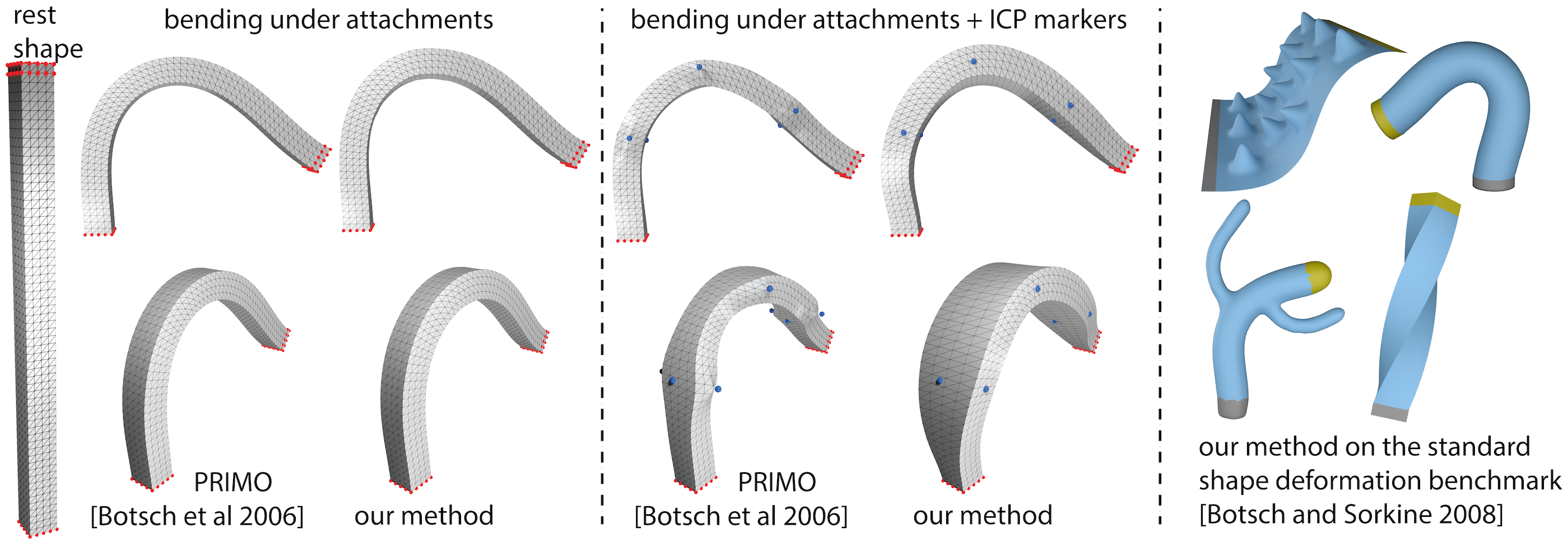
Finally, we note that our formulation is different to approaches that optimize the deformation gradient directly (i.e., without an intermediary quantity such as the plastic deformation gradient). In Figures 4 and 7, we compare to two such approaches: deformation transfer (Sumner and Popović 2004) and variational shape modeling (Botsch and Kobbelt 2004). We demonstrate that our method better captures shapes defined using our inputs (landmarks, ICP markers, large spatially varying strains). Among all compared approaches, the variational method in Figure 7 came closest to meeting our constraints, but there is still a visual difference to our method. We provide a further comparison to variational methods in Section 4.5.

3.4. Solving the optimization problem for attached objects

We adapt the Gauss-Newton method (Sifakis et al. 2005) to efficiently solve the optimization problem of Equations 3 and 4 (example output shown in Figure 6). Doing so is not straightforward because a direct application of the Gauss-Newton method results in large dense matrices that are costly to compute and store, causing the method to fail on complex examples. Below, we demonstrate how to avoid these issues, producing a robust method capable of handling complex spatially varying plastic strains. Before settling on our specific Gauss-Newton approach, we also attempted to use the interior-point optimizer available in the state-of-the-art Knitro optimization library (Artelys 2019). This did not work well because our problem is highly nonlinear. The interior-point method (IPM) worked well on simple examples, but was slow and not convergent on complex examples. IPM fails because it requires the constraint Hessian, which is not available. When we approximated it, IPM generated intermediate states too far from the constraints, and failed. The strength of our Gauss-Newton approach is that we only need constraint gradients. Our method inherits the convergence properties of the Gauss-Newton method. While not guaranteed to be locally convergent, Gauss-Newton is widely used because its convergence can approach quadratic when close to the solution.
We note that our method is designed for sparse medical image landmarks and ICP markers. In Figure 8, we give a comparison to a related method from medical imaging which used an elastic energy, but with dense correspondences. Our method can produce a quality shape even under sparse inputs, and can consequently work even with coarser MRI scans (such as our hip bone example; Figure 13). The ability to work with sparse markers also translates to lower manual processing time to select the markers in the medical image.
Because the object is attached, Equation 4 implicitly defines as a function of The Gauss-Newton method uses the Jacobian which models the change in the static equilibrium as one changes the plastic deformation gradient. It eventually relies on the derivative of elastic forces with respect to the plastic deformation gradient, which we give in Appendix B. Because and are quadratic functions of we rewrite Equations 3 and 4 as
| (6) | |||
| (7) |
where is the net force on the mesh, and constant matrices, vectors and scalars are independent of and (we give them in Appendix F). The integer denotes the number of attachments. We now re-write Equations 6 and 7 so that the plastic strains are expressed as and the equilibrium as where At iteration of our Gauss-Newton method, given the previous iterates and we minimize a nonlinearly constrained problem,
| (8) | |||
| (9) |
After each iteration, we update Observe that Equation 8 does not depend on and that the constraint of Equation 9 is already differentially “baked” into Equation 8 via We therefore first minimize Equation 8 for using unconstrained minimization; call the solution A naive minimization requires solving a large dense linear system of equations, which we avoid using the technique presented at the end of this section. We regularize so that the corresponding is always positive-definite for each tet; we do this by performing eigen-decomposition of the symmetric matrix at each tet, and clamping any negative eigenvalues to a small positive value (we use 0.01). Our method typically did not need to perform clamping in practice, and in fact such clamping is usually a sign that the method is numerically diverging, and should be restarted with better parameter values.
We then minimize the optimization problem of Equations 8 and 9 using a 1D line search, using the search direction Specifically, for we first solve Equation 7 with for using the Knitro library (Artelys 2019). Direct solutions using a Newton-Raphson solver also worked, but we found Knitro to be faster. We then evaluate the objective of Equation 6 at and We perform the 1D line search for the optimal using the Brent’s method (Press et al. 2007) because it does not require a gradient.
Initial guess:
We solve our optimization problem by first assuming a constant at each tet, starting from the template mesh as the initial guess. This roughly positions, rotates and globally scales the template mesh to match the medical image. We use the output as the initial guess for our full optimization as described above.

Optimization stages and stopping criteria:
We first do the optimization with attachments only. Upon convergence, we add the landmarks, ignoring any ICP markers. This is because initially, the mesh is far away from the target and the ICP closest locations are unreliable. After convergence, we disable the landmarks and enable the ICP markers and continue optimizing. After this optimization meets a stopping criterium, we are done. Our output is therefore computed with ICP markers only; landmarks only serve to guide the optimizer. This is because landmarks require a correct correspondence, and it is harder to mark this correspondence reliably in the scan than to simply select an ICP marker on the boundary of an organ. We recompute the closest locations to ICP markers after each Gauss-Newton iteration. We stop the optimization if either of the following three criteria is satisfied: (i) reached the user-specified maximal number of iterations (typically 20; but was as high as 80 in the liver example), (ii) maximum error at ICP markers is less than a user-specified value (1mm for hand muscles), (iii) the progress in each iteration is too small, determined by checking if is under a user-defined threshold (we use 0.01). Figure 9 shows the convergence of our optimization.
Avoiding dense large linear systems
Because the object is attached, is square and invertible. Therefore, one can obtain a formula for by differentiating Equation 7 with respect to
| (10) |
The matrix is dense (dimensions ). Observe that because Equation 8 is quadratic in minimizing it as done above to determine the search direction is equivalent to solving a linear system with the system matrix where is the second derivative (Hessian matrix; dimension ) of Equation 8 with respect to Because is dense, is likewise a dense matrix,
| (11) | |||
| (12) |
Therefore, when the number of tet mesh elements is large, it is not practically possible to compute store it explicitly in memory or solve linear systems with it. To avoid this problem, we first tried solving the system of equations using the Conjugate Gradient (CG) method. This worked, but was very slow (Table 1). The matrix is dense. In our complex examples, the number of medical image constraints is small (typically 10 - 800) compared to the dimension of (; typically ~200,000). Our idea is to efficiently compute the solution to a system for any right-hand side using the Woodbury matrix identity (Woodbury 1950), where we view as a “base” matrix and a low-rank perturbation. Before we can apply Woodbury’s identity, we need to ensure that the base matrix is invertible. As we prove in Appendix A, the plastic strain Laplacian is singular with six orthonormal vectors in its nullspace (assuming that is connected). Each is a vector of all ones in component of and all zeros elsewhere, divided by for normalization. It follows from the Singular Lemma (i) (Section 3.5) that is also singular with the same nullspace vectors. Therefore, we decompose
| (13) |
where and is matrix with an additional added 6 added rows By the Singular Lemma (iii) (Section 3.5), is now invertible, and we can use Woodbury’s identity to solve
| (14) |
We rapidly compute without ever computing or forming by solving sparse systems for Observe that this sparse system matrix is symmetric and the same for all We factor it once using the Pardiso solver and then solve the multiple right-hand sides in parallel. The matrix is constant, and we only need to factor it once for the entire optimization. Finally, the matrix is small, and so inverting it is fast. We analyze the performance of our algorithm in Table 1.
| Example | CG | Ours | |||
|---|---|---|---|---|---|
| Hand muscle | 237,954 | 1,143 | 17.5s | 897.5s | 9.5s |
| Hip bone | 172,440 | 1,497 | 11.4s | 408.9s | 7.2s |
| Liver | 259,326 | 1,272 | 24.4s | 1486.7s | 10.0s |
3.5. Singular lemma

In this paper, there are two occasions where we have
to solve a singular sparse linear system with known nullspace
vectors. Such systems occur often in modeling of un-attached
objects, e.g., finding static equilibria,
solving Laplace equations on the object’s mesh,
animating with rotation-strain coordinates (Huang
et al. 2011),
or computing modal derivatives (Barbič and
James 2005).
Previous work solved such systems ad-hoc, and the underlying theory has not been
stated or developed in any great detail. We hereby state and prove a lemma that comprehensively
surveys the common situations arising with singular systems in computer animation and simulation,
and back the lemma with a mathematical proof (Appendix C).
Recall that the nullspace of a matrix
is ,
and the range of is
Both are linear vector subspaces of
Singular Lemma:
Let the square symmetric matrix be singular with
a known nullspace spanned by linearly independent
vectors Then the following statements hold:
(i) and are orthogonal.
Every vector can be uniquely expressed as
where
and Vector is orthogonal to
and to for all (Figure 10).
(ii) Let Then, the singular system has
a unique solution
with the property that is orthogonal
to for all
This solution can be found by solving the non-singular linear system
| (15) |
All other solutions equal
for some scalars
(iii) For any scalars the matrix
is invertible. If
are orthonormal vectors, then
the solution to
equals
where and are solutions to Equation 15
with
We give the proof of the singular lemma in Appendix C.
3.6. Un-attached objects


The difficulty with un-attached objects is that we now have and the equation no longer has a unique solution for a fixed plastic state This can be intuitively easily understood: one can arbitrarily translate and rotate any elastic equilibrium shape under the given plastic state doing so produces another elastic equilibrium shape. The space of solutions is 6-dimensional. This means that we can no longer uniquely solve Equation 7 for during our line search of Section 3.4. Furthermore, the square tangent stiffness matrix
| (16) |
is no longer full rank.
In order to address this, we now state and prove the following Nullspace Lemma.
Nullspace Lemma: The nullspace of the tangent stiffness matrix of an elastoplastic deformable object in static equilibrium under plasticity, is 6-dimensional. The six nullspace vectors are where is the -th standard basis vector, and for
To the best of our knowledge, this fact of elasto-plasto-statics has not been stated or proven in prior work. It is very useful when modeling large-deformation elastoplasticity, as real objects are often un-attached, or attachments cannot be easily modeled. We give a proof in Appendix D. To accommodate un-attached objects, it is therefore necessary to stabilize the translation and rotation. For translations, this could be achieved easily by fixing the position of any chosen vertex. Matters are not so easy for rotations, however. Our idea is to constrain the centroid of all tet mesh vertices to a specific given position and to constrain the “average rotation” of the model to a specific given rotation We achieve this using the familiar “shape-matching” (Müller et al. 2005), by imposing that the rotation in the polar decomposition of the global covariance matrix must be We therefore solve the following optimization problem,
| (17) | |||
| (18) | |||
| (19) | |||
| (20) |
where is the set of points on the mesh surface where we have either a landmark or an ICP constraint, is the weight of a point, is the position of vertex in and is the polar decomposition function that extracts the rotational part of a matrix We set all weights equal, i.e., We choose the set as opposed to all mesh vertices so that we can easily perform optimization with respect to and (next paragraph). We assume that our argument matrices to are not inversions, i.e., which establishes that is always a rotation and not a mirror. This requirement was easily satisfied in our examples, and is essentially determined by the medical imaging constraints; the case would correspond to an inverted (or mirror) medical image, which we exclude.
We solve the optimization problem of Equations 17, 18, 19 and 20 using a block-coordinate descent, by iteratively optimizing while keeping fixed and vice-versa (Figure 11, 12). Rigid transformations do not affect smoothness of so we do not need to consider it when optimizing We need to perform two modifications to our Gauss-Newton iteration of Section 3.4. The first modification is that we need to simultaneously solve Equations 18, 19 and 20 when determining the static equilibrium in the current plastic state As with attached objects, we do this using the Knitro optimizer. In order to do this, we need to compute the first and second derivatives of the stabilization constraints in Equations 19 and 20 (Section 3.7). The second modification is needed because the tangent stiffness matrix as explained above, is now singular with a known 6-dimensional nullspace. In order to compute the Jacobian matrix using Equation 10, we use our Singular Lemma (ii) (Section 3.5). Note that the right-hand side is automatically in the range of because Equation 10 was obtained by differentiating a valid equation, hence Equation 10 must also be consistent.
3.7. Gradient and Hessian of
Previous work computed first and second-order time derivatives of the rotation matrix in polar decomposition (Barbič and Zhao 2011), or first derivative with respect to each individual entry of (Twigg and Kačić-Alesić 2010; Chao et al. 2010). In our work, we need the first and second derivatives of with respect to each individual entry of We found an elegant approach to compute them using Sylvester’s equation, as follows. Observe that where is the symmetric matrix in the polar decomposition. Because is positive-definite and uniquely defined as To compute the first-order derivatives, we start from , and differentiate,
| (21) |
Therefore, we need to compute We have
| (22) |
i.e., this is the classic Sylvester equation for the unknown matrix (Sylvester 1884). The Sylvester equation can be solved as
| (23) |
where is the Kronecker sum of two matrices. In our case,
| (24) |
The computation of second-order derivatives follows the same recipe: differentiate the polar decomposition and solve a Sylvester equation. We give it in Appendix E.
We can now compute the gradient and Hessian of our stabilization constraints. The translational constraint is linear in and can be expressed as where is a sparse matrix. Although is not linear, the argument of is linear in The rotational constraint can be expressed as where is a sparse matrix. The Jacobian of the translational constraint is and the Hessian is zero. For the rotational constraint, the Jacobian is and the Hessian is where denotes tensor contraction.


3.8. Comparison to standard shape deformation methods
Our shape deformation setup is similar to standard shape deformation problems in computer graphics. In fact, we first attempted to solve the shape deformation problem with as-rigid-as-possible energy (ARAP) (Sorkine and Alexa 2007), bounded biharmonic weights (BBW) (Jacobson et al. 2011), biharmonic weights with linear precision (LBW) (Wang et al. 2015a), and a Finite Element Method static solver (FEM) (Barbič et al. 2009). Unfortunately, none of the methods worked well. Figures 14 and 15 demonstrate that these methods produce non-smooth shapes with spikes (ARAP, BBW, FEM), or wiggles (LBW).
Mathematically, the reason for the spikes in ARAP, BBW and FEM is that point constraints for second-order methods are inherently flawed. As one refines the solution by adding more tetrahedra, the solution approaches a spiky point function at each point constraint, which is obviously not desirable. This mathematical issue is exposed in our work because our shape deformation consists of large spatially varying stretches. Often, the template mesh needs to be stretched 2x or more along some (or several) coordinate axes. The medical image constraints are distributed all around the muscle, pulling in different directions and essentially requesting the object to undergo a spatially non-uniform and anisotropic scale. This exacerbates the spikiness for second-order methods. We note that these problems cannot be avoided simply by using an elastic energy that permits volume growth. Namely, Drucker’s stability condition (Drucker 1957) requires a monotonic elastic energy increase with increase in strain. An elastic energy therefore must penalize strain increases if it is to be stable; and this impedes large-strain modeling in methods that rely purely on an elastic energy. Our plasticity method does not penalize large strains and thus avoids this problem. Spikes can be avoided by using a higher-order variational method such as LBW. However, our experiments indicate that such methods suffer from wiggles when applied to medical imaging problems (see also Figures 7 and 23).
4. Results
We extracted muscles of the human hand and the hip muscle from an MRI scan, and a hip bone and a liver from a CT scan. We analyze the performance of our method in Table 2. In Figure 16, we give histograms of the magnitude of the difference between the positions of the medical image markers and their output positions. It can be seen that our method produces shapes that generally match the medical image constraints to 0.5mm or better. In Figure 17, we demonstrate that the output quality of our tetrahedra is still good; if needed, this could be further improved by re-meshing (Bargteil et al. 2007). Figures 18 and 19 superimpose our output meshes on the CT and MRI scans, respectively. In Figure 20, we compare to a recent implicit point set surface reconstruction method (Huang et al. 2019). In Figure 21, we evaluate our method in the presence of known ground truth plastic deformation gradients. Figure 22 provides a comparison to surface-based methods.
| Example | # vtx | # ele | # markers | # iter | time [min] | attached | ||
|---|---|---|---|---|---|---|---|---|
| Hand muscle (min) | 4,912 | 20,630 | 15 | 8 | 14.2 | yes | 0.53 / 2.22 | 0.06 / 0.14 |
| Hand muscle (med) | 6,260 | 31,737 | 32 | 12 | 12.8 | yes | 0.62 / 1.56 | 0.11 / 0.55 |
| Hand muscle (max) | 8,951 | 42,969 | 96 | 11 | 14.2 | yes | 3.35 / 12.82 | 0.11 / 0.34 |
| Hand muscle (max-m) | 7,552 | 34,966 | 151 | 18 | 20.3 | yes | 3.28 / 9.11 | 0.16 / 0.47 |
| Hip muscle (Fig 13) | 6,793 | 34,118 | 82 | 21 | 28.3 | yes | 7.41 / 21.27 | 0.39 / 1.85 |
| Hip bone | 6,796 | 28,740 | 499 | 34 | 49.2 | no | 4.12 / 14.27 | 0.25 / 1.30 |
| Liver | 11,392 | 43,221 | 424 | 80 | 128.3 | no | 9.00 / 33.68 | 0.21 / 4.81 |
| Hand surface (Fig 15) | 11,829 | 49,751 | 456 | 31 | 43.8 | no | 4.87 / 16.78 | 0.07 / 0.86 |


4.1. Hand muscles
In our muscle hand example, we extracted 17 hand muscles from an MRI scan (Figure 6). We obtained the scan and the already extracted bone meshes from (Wang et al. 2019); scan resolution is 0.5mm x 0.5mm x 0.5mm . We considered two “templates”, the first one from the Centre for Anatomy and Human Identification at the University of Dundee, Scotland (C. Erolin 2019), and the second one from Zygote (Zygote 2016). We used the first one (Figure 6, left) because we found it to be more medically accurate (muscles insert to correct bones). Muscle anatomy of a human hand is challenging (Figure 6). We model all muscle groups of the hand, namely the thenar eminence (thumb), hypothenar eminence (below little finger), interossei muscles (palmar and dorsal) (between metacarpal bones), adductor pollicis (soft tissue next to the thumb, actuating thumb motion), and lumbricals (on the side of the fingers at the fingers base). Our template models the correct number and general location of the muscles, but there are large muscle shape differences between the template subject and the scanned subject (Figure 1). We solve the optimization problem of Equations 3 and 4 separately for each muscle, starting from the template mesh as the initial guess. In our results, this produces muscles that match the attachments and medical image constraints markers at 0.5 mm or better, which is at, or better than, the accuracy of the MRI scanner.
4.1.1. Marking the muscles in MRI scans
During pre-processing, we manually mark as many reliable points as possible on the boundary of each muscle ( landmarks and ICP markers per muscle) in the MRI scans. This process took approximately 5 minutes per muscle.
4.1.2. Attachments to bones
The template muscles are modeled as triangle meshes. We build a tetrahedral mesh for each muscle. Our tet meshes conform to the muscle’s surface triangle mesh; this requirement could be relaxed. For each muscle in the template, we attach its tet mesh to the bones using soft constraints. We do this by marking where on one or multiple bones this muscle inserts; to do so, we consulted a medical doctor with specific expertise in anatomy. For each bone triangle mesh vertex that participates in the insertion, we determine the material coordinates (i.e., tet barycentric coordinates) in the closest muscle tet. We then form a soft constraint whereby this muscle material point is linked to the bone vertex position using a spring.
4.1.3. Direct attempt using segmentation:
We note that we have also attempted to model the muscle shapes directly using segmentation, simply from an MRI scan. Recent work has demonstrated that this can be done for hand bones (Wang et al. 2019), and we attempted a similar segmentation approach for muscles. However, given that the muscles touch each other in many places (unlike bones), the contrast in the MRI scan was simply not sufficient to discern the individual muscles. Our conclusion is that a segmentation approach is not feasible for hand muscles, and one must use a pre-existing anatomically accurate template as in our work.
4.1.4. Removing inter-penetrations of muscles

Many hand muscles are in close proximity to one another and several are in continuous contact. One strategy to resolve contact would be to incorporate contact into our optimization (Equations 3 and 4). This approach is not very practical, as unilateral constraints are very difficult to optimize. Furthermore, such an approach couples all (or most) muscles, and requires one to solve an optimization problem with a much larger number of degrees of freedom. It is extremely slow at our resolution; it overpowers our machine. Instead, we optimize each muscle separately. Of course, the different muscles inter-penetrate each other, which we resolve as follows. For each muscle, we already positioned the MRI constraints so that they are at the muscle boundary. Therefore, observe that if our marker positioning and the solution to the optimization problem were perfect, inter-penetration would be minimal or non-existent. The marker placement is relatively straightforward at the boundary between a muscle and another tissue (bone, fat, etc.) due to good contrast. However, placing markers at the boundary between two continuously colliding muscles is less precise, due to a lower MRI contrast between adjacent muscles. This is the main cause of the inter-penetrations. We remove the inter-penetrations with FEM simulation because it produces smooth organic shape changes; note that alternatively, geometric approaches could also be used (Schmid et al. 2009). Specifically in our work, for a pair of inter-penetrating muscles, we run collision detection to determine the set of triangles of each muscle that are inside the volume of the other muscle. On each muscle, we then determine the set of tetrahedra that are adjacent to the collision area. We then slightly enlarge this set, by including any tet within a 5-ring of tets. We then run a FEM contact simulation just on these two tetrahedral sets on the two muscles. The FEM simulation pushes the muscle surface boundaries apart, without displacing the rest of the muscle (Figure 19). We handle contact islands of multiple muscles by running the above procedure on two muscles, then for a third muscle against the first two muscles, then the fourth against the first three, and so on.
4.2. Hip bone
In our second anatomical example (Figure 11), we apply our method to a CT scan of the human right hip bone (pelvis). We obtained the template from the human anatomy model of Ziva Dynamics (Ziva Dynamics 2019), and the CT scan from the “KidneyFullBody” medical image repository (Stephcavs 2019). The template and the scanned hip bone differ substantially in shape, and this is successfully captured by our method.
4.3. Liver
In our third anatomical example, we apply our method to a CT scan of the human liver (Figure 12). We purchased a textured liver triangle mesh on TurboSquid (Turbosquid 2019). We subdivided it and created a tet mesh using TetGen (Hang Si 2011). This serves as our “template”. We used a liver CT scan from the “CHAOS” medical image repository (Kavur et al. 2019). We then executed our method to reshape the template tet mesh to match the CT scan. Much like with the hip bone, our method successfully models the large differences between the template and the scanned liver. Finally, we embedded the TurboSquid triangle mesh into the template tet mesh, and transformed it with the shape deformation of the tet mesh. This produced a textured liver mesh (Figure 12) that matches the CT scan.
4.4. Hip muscle
In our fourth anatomical example, we apply our method to a MRI scan of a female human hip muscle (gluteus medius) (Figure 13). We obtained the data from The Cancer Imaging Archive (TCIA) (Clark et al. 2013). The image resolution is with voxel spacing of 1mm, which is 2x coarser to the hand MRI dataset. We use the template mesh from the human anatomy model of Ziva Dynamics (Ziva Dynamics 2019). We subdivided it and created a tet mesh for it using TetGen (Hang Si 2011). Because the muscle is attached to the hip bone and the leg bone, we needed to first extract the bones from the MRI scan; we followed the method described in (Wang et al. 2019). Note that the subject in the Ziva Dynamics template is male. The template and the scanned hip muscle differ substantially in shape, and this is successfully captured by our method.


4.5. Comparison to variational methods
We compare our method to variational shape modeling methods on an illustrative 1D example. Note that Figure 7 gave a comparison on 3D muscle geometry. Consider an elastic 1D line segment whose neutral shape is the interval and study its longitudinal 1D deformation under the following setup. Let us prescribe hard attachments whereby we attach endpoint to position and endpoint to position Furthermore, assume landmarks whereby point is at and point is at Effectively in this setup, we are specifying that the subintervals and do not stretch, whereas the subinterval stretches from its original length of to (5x stretch). A variational formulation of order is,
| (25) |
where denotes all functions whose derivatives exist and are continuous up to order We solved these problems analytically in Mathematica for each time for three representative values and compared them (see Figure 23) to our method in 1D,
| (26) | |||
| (27) |
Observe that, in the same vein as in 3D, we can decompose whereby scalar functions and and the term are the equivalents of the elastic and plastic deformation gradients, and the elastic energy, respectively. It can be seen that our method produces a better fit to the data and a significantly less wiggly solution, compared to variational methods (Figure 23).

5. Conclusion
We gave a shape deformation method that can model objects undergoing large spatially varying strains. Our method works by computing a plastic deformation gradient at each tet, such that the mesh deformed by these plastic deformation gradients matches the provided sparse landmarks and closest-point constraints. We support both constrained and unconstrained objects; the latter are supported by giving a numerical method to solve large sparse linear systems of equations with a known nullspace. We applied our method to the extraction of shapes of organs from medical images. Our method has been designed to extract as much information as possible from MRI images, despite the soft boundaries between the different organs. We extracted hand muscles, a liver, a hip bone and a hip muscle.
Our method does not require a dense target mesh; only a sparse set of observations is needed. If a dense target mesh is available, the problem becomes somewhat easier, as one can then use standard ICP algorithms. However, medical images contain many ambiguities and regions where there is not a sufficient contrast to clearly disambiguate two adjacent medical organs; making it impractical to extract dense target meshes. We apply our method to solid objects, but our plastic strain shape deformation method could also be used for shells (cloth). Doing so would require formulating the elastic energy of a plastically deformed FEM cloth, and computing the energy gradients and Hessians with respect to the plastic parameters. The size of the small square dense matrix that we need to invert in our incremental solve is three times the number of markers. While we easily employed up to a thousand of markers in our work, our method will slow down under a large number of markers. We do not re-mesh our tet meshes during the optimization. If the plastic strain causes some tetrahedra to collapse or nearly collapse, this will introduce numerical instabilities. Although not a problem in our examples (see Figure 17), such situations could be handled by re-meshing the tet mesh during the optimization (Bargteil et al. 2007). Our method requires a plausible template with a non-degenerate tet mesh. Re-meshing is important future work as it could extend the reach of our method, enabling one to start the optimization simply from a sphere tet mesh.
References
- (1)
- Alexa et al. (2006) M. Alexa, A. Angelidis, M.-P. Cani, S. Frisken, K. Singh, S. Schkolne, and D. Zorin. 2006. Interactive Shape Modeling. In ACM SIGGRAPH 2006 Courses. 93.
- Artelys (2019) Artelys. 2019. Knitro. https://www.artelys.com/solvers/knitro/.
- Barbič et al. (2009) J. Barbič, M. da Silva, and J. Popović. 2009. Deformable Object Animation Using Reduced Optimal Control. ACM Trans. on Graphics 28, 3 (2009).
- Barbič and James (2005) J. Barbič and D. L. James. 2005. Real-time subspace integration for St. Venant-Kirchhoff deformable models. ACM Trans. on Graphics 24, 3 (2005), 982–990.
- Barbič and Zhao (2011) J. Barbič and Y. Zhao. 2011. Real-time Large-deformation Substructuring. ACM Trans. on Graphics (SIGGRAPH 2011) 30, 4 (2011), 91:1–91:7.
- Bargteil et al. (2007) A. W. Bargteil, C. Wojtan, J. K. Hodgins, and G. Turk. 2007. A finite element method for animating large viscoplastic flow. In ACM Transactions on Graphics (SIGGRAPH 2007), Vol. 26. 16.
- Bergou et al. (2007) Miklós Bergou, Saurabh Mathur, Max Wardetzky, and Eitan Grinspun. 2007. TRACKS: Toward directable thin shells. ACM Trans. on Graphics (SIGGRAPH 2007) 26, 3 (2007), 50:1–50:10.
- Botsch and Kobbelt (2004) Mario Botsch and Leif Kobbelt. 2004. An Intuitive Framework for Real-Time Freeform Modeling. ACM Trans. on Graphics (SIGGRAPH 2004) 23, 3, 630–634.
- Botsch et al. (2006) Mario Botsch, Mark Pauly, Markus Gross, and Leif Kobbelt. 2006. PriMo: Coupled Prisms for Intuitive Surface Modeling. In Eurographics Symp. on Geometry Processing. 11–20.
- Botsch and Sorkine (2008) M. Botsch and O. Sorkine. 2008. On linear variational surface deformation methods. IEEE Trans. on Vis. and Computer Graphics 14, 1 (2008), 213–230.
- C. Erolin (2019) C. Erolin. 2019. Hand Anatomy. University of Dundee, Centre for Anatomy and Human Identification. https://sketchfab.com/anatomy_dundee/collections/hand-anatomy.
- Chao et al. (2010) I. Chao, U. Pinkall, P. Sanan, and P. Schröder. 2010. A Simple Geometric Model for Elastic Deformations. ACM Transactions on Graphics 29, 3 (2010), 38:1–38:6.
- Chen et al. (2018) W. Chen, F. Zhu, J. Zhao, S. Li, and G. Wang. 2018. Peridynamics-Based Fracture Animation for Elastoplastic Solids. In Computer Graphics Forum, Vol. 37. 112–124.
- Clark et al. (2013) K. Clark, B. Vendt, K. Smith, J. Freymann, J. Kirby, P. Koppel, S. Moore, S. Phillips, D. Maffitt, M. Pringle, L. Tarbox, and F. Prior. 2013. The Cancer Imaging Archive (TCIA): maintaining and operating a public information repository. J Digit Imaging 26, 6 (Dec 2013), 1045–1057.
- Dicko et al. (2013) Ali Hamadi Dicko, Tiantian Liu, Benjamin Gilles, Ladislav Kavan, Francois Faure, Olivier Palombi, and Marie-Paule Cani. 2013. Anatomy Transfer. ACM Trans. on Graphics (SIGGRAPH 2013) 32, 6 (2013), 188:1–188:8.
- Drucker (1957) Daniel Charles Drucker. 1957. A definition of stable inelastic material. Technical Report. DTIC Document.
- Gilles and Magnenat-Thalmann (2010) B. Gilles and N. Magnenat-Thalmann. 2010. Musculoskeletal MRI segmentation using multi-resolution simplex meshes with medial representations. Med. Image Anal. 14, 3 (2010), 291–302.
- Gilles et al. (2006) Benjamin Gilles, Laurent Moccozet, and Nadia Magnenat-Thalmann. 2006. Anatomical Modelling of the Musculoskeletal System from MRI. In Medical Image Computing and Computer-Assisted Intervention – MICCAI 2006. 289–296.
- Gilles et al. (2010) Benjamin Gilles, Lionel Reveret, and Dinesh Pai. 2010. Creating and animating subject-specific anatomical models. Computer Graphics Forum 29, 8 (2010), 2340–2351.
- Grady (2006) Leo Grady. 2006. Random walks for image segmentation. IEEE Trans. on Pattern Analysis and Machine Intelligence 28, 11 (2006), 1768–1783.
- Hang Si (2011) Hang Si. 2011. TetGen: A Quality Tetrahedral Mesh Generator and a 3D Delaunay Triangulator.
- Huang et al. (2011) Jin Huang, Yiying Tong, Kun Zhou, Hujun Bao, and Mathieu Desbrun. 2011. Interactive Shape Interpolation through Controllable Dynamic Deformation. IEEE Trans. on Visualization and Computer Graphics 17, 7 (2011), 983–992.
- Huang et al. (2019) Z. Huang, N. A. Carr, and T. Ju. 2019. Variational implicit point set surfaces. ACM Trans. on Graphics (SIGGRAPH 2019) 38, 4 (2019).
- Ichim et al. (2017) A.E. Ichim, P. Kadlecek, L. Kavan, and M. Pauly. 2017. Phace: Physics-based Face Modeling and Animation. ACM Trans. on Graphics (SIGGRAPH 2017) 36, 4 (2017).
- Igarashi et al. (2005) T. Igarashi, T. Moscovich, and J. F. Hughes. 2005. As-rigid-as-possible shape manipulation. ACM Trans. on Graphics (SIGGRAPH 2005) 24, 3 (2005), 1134–1141.
- Irving et al. (2004) G. Irving, J. Teran, and R. Fedkiw. 2004. Invertible Finite Elements for Robust Simulation of Large Deformation. In Symp. on Computer Animation (SCA). 131–140.
- Jacobson et al. (2011) A. Jacobson, I. Baran, J. Popović, and O. Sorkine. 2011. Bounded biharmonic weights for real-time deformation. ACM Trans. on Graphics (TOG) 30, 4 (2011), 78.
- Kadlecek et al. (2016) Petr Kadlecek, Alexandru-Eugen Ichim, Tiantian Liu, Jaroslav Krivanek, and Ladislav Kavan. 2016. Reconstructing Personalized Anatomical Models for Physics-based Body Animation. ACM Trans. Graph. 35, 6 (2016).
- Kavan et al. (2011) Ladislav Kavan, Dan Gerszewski, Adam W. Bargteil, and Peter-Pike Sloan. 2011. Physics-Inspired Upsampling for Cloth Simulation in Games. ACM Trans. Graph. 30, 4, Article 93 (2011), 10 pages.
- Kavur et al. (2019) Ali Emre Kavur, M. Alper Selver, Oǧuz Dicle, Mustafa Bariş, and N. Sinem Gezer. 2019. CHAOS - Combined (CT-MR) Healthy Abdominal Organ Segmentation Challenge Data. https://doi.org/10.5281/zenodo.3362844
- Kazhdan and Hoppe (2013) Michael Kazhdan and Hugues Hoppe. 2013. Screened Poisson Surface Reconstruction. ACM Trans. on Graphics (TOG) 32, 3, Article 29 (2013).
- Lee et al. (2018) Seunghwan Lee, Ri Yu, Jungnam Park, Mridul Aanjaneya, Eftychios Sifakis, and Jehee Lee. 2018. Dexterous manipulation and control with volumetric muscles. ACM Transactions on Graphics (SIGGRAPH 2018) 37, 4 (2018), 57:1–57:13.
- Lee et al. (2009) S. H. Lee, E. Sifakis, and D. Terzopoulos. 2009. Comprehensive Biomechanical Modeling and Simulation of the Upper Body. ACM Trans. on Graphics 28, 4 (2009), 99:1–99:17.
- McInerney and Terzopoulos (2008) T. McInerney and D. Terzopoulos. 2008. Deformable Models. In Handbook of Medical Image Processing and Analysis (2nd Edition), I. Bankman (Ed.). Chapter 8, 145–166.
- Müller and Gross (2004) M. Müller and M. Gross. 2004. Interactive Virtual Materials. In Proc. of Graphics Interface 2004. 239–246.
- Müller et al. (2005) M. Müller, B. Heidelberger, M. Teschner, and M. Gross. 2005. Meshless Deformations Based on Shape Matching. In Proc. of ACM SIGGRAPH 2005. 471–478.
- Niculescu et al. (2009) G. Niculescu, J.L. Nosher, M.D. Schneider, and D.J. Foran. 2009. A deformable model for tracking tumors across consecutive imaging studies. Int. J. of Computer-Assisted Radiology and Surgery 4, 4 (2009), 337–347.
- O’Brien et al. (2002) James F. O’Brien, Adam W. Bargteil, and Jessica K. Hodgins. 2002. Graphical Modeling and Animation of Ductile Fracture. In Proceedings of ACM SIGGRAPH 2002. 291–294.
- Press et al. (2007) W. Press, S. Teukolsky, W. Vetterling, and B. Flannery. 2007. Numerical recipes: The art of scientific computing (third ed.). Cambridge University Press, Cambridge, UK.
- Rhee et al. (2011) T. Rhee, U. Neumann, J. Lewis, and K. S. Nayak. 2011. Scan-Based Volume Animation Driven by Locally Adaptive Articulated Registrations. IEEE Trans. on Visualization and Computer Graphics 17, 3 (2011), 368–379.
- Saito et al. (2015) Shunsuke Saito, Zi-Ye Zhou, and Ladislav Kavan. 2015. Computational Bodybuilding: Anatomically-based Modeling of Human Bodies. ACM Trans. on Graphics (SIGGRAPH 2015) 34, 4 (2015).
- Schmid et al. (2011) J. Schmid, E. Gobbetti J. A. I. Guitián, and N. Magnenat-Thalmann. 2011. A GPU framework for parallel segmentation of volumetric images using discrete deformable models. The Visual Computer 27 (2011), 85–95.
- Schmid and Magnenat-Thalmann (2008) Jérôme Schmid and Nadia Magnenat-Thalmann. 2008. MRI Bone Segmentation Using Deformable Models and Shape Priors. In Medical Image Computing and Computer-Assisted Intervention – MICCAI 2008. 119–126.
- Schmid et al. (2009) J. Schmid, A. Sandholm, F. Chung, D. Thalmann, H. Delingette, and N. Magnenat-Thalmann. 2009. Musculoskeletal Simulation Model Generation from MRI Data Sets and Motion Capture Data. Recent Advances in the 3D Physiological Human (2009), 3–19.
- Sifakis et al. (2005) Eftychios Sifakis, Igor Neverov, and Ronald Fedkiw. 2005. Automatic determination of facial muscle activations from sparse motion capture marker data. ACM Trans. on Graphics (SIGGRAPH 2005) 24, 3 (Aug. 2005), 417–425.
- Smith et al. (2018) Breannan Smith, Fernando De Goes, and Theodore Kim. 2018. Stable Neo-Hookean Flesh Simulation. ACM Trans. Graph. 37, 2 (2018), 12:1–12:15.
- Sorkine and Alexa (2007) Olga Sorkine and Marc Alexa. 2007. As-rigid-as-possible surface modeling. In Symp. on Geometry Processing, Vol. 4. 109–116.
- Sorkine et al. (2004) O. Sorkine, D. Cohen-Or, Y. Lipman, M. Alexa, C. Rössl, and H-P Seidel. 2004. Laplacian surface editing. In Symp. on Geometry processing. 175–184.
- Stephcavs (2019) Stephcavs. 2019. KidneyFullBody 1.0.0: Full CT scan of body. https://www.embodi3d.com/files/file/26389-kidneyfullbody/.
- Stomakhin et al. (2013) A. Stomakhin, C. Schroeder, L. Chai, J. Teran, and A. Selle. 2013. A Material Point Method for Snow Simulation. ACM Trans. on Graphics (SIGGRAPH 2013) 32, 4 (2013), 102:1–102:10.
- Sumner and Popović (2004) Robert W Sumner and Jovan Popović. 2004. Deformation transfer for triangle meshes. ACM Trans. on Graphics (SIGGRAPH 2004) 23, 3 (2004), 399–405.
- Sylvester (1884) J. Sylvester. 1884. Sur l’equations en matrices p x = x q. C. R. Acad. Sci. Paris. 99, 2 (1884), 67–71, 115–116.
- Székely et al. (1996) G. Székely, A. Kelemen, C. Brechbühler, and G. Gerig. 1996. Segmentation of 2-D and 3-D objects from MRI volume data using constrained elastic deformations of flexible Fourier contour and surface models. Medical Image Analysis 1, 1 (1996), 19–34.
- Tissue (2013) Tissue. 2013. Weta Digital: Tissue Muscle and Fat Simulation System.
- Turbosquid (2019) Turbosquid. 2019. www.turbosquid.com.
- Turk and O’Brien (1999) G. Turk and J. O’Brien. 1999. Shape transformation using variational implicit functions. In Proc. of ACM SIGGRAPH 1999. 335–342.
- Twigg and Kačić-Alesić (2010) C. Twigg and Z. Kačić-Alesić. 2010. Point Cloud Glue: constraining simulations using the procrustes transform. In Symp. on Computer Animation (SCA). 45–54.
- Twigg and Kačić-Alesić (2011) Christopher D. Twigg and Zoran Kačić-Alesić. 2011. Optimization for Sag-Free Simulations. In Proc. of the 2011 ACM SIGGRAPH/Eurographics Symp. on Computer Animation. 225–236.
- U.S. National Library of Medicine (1994) U.S. National Library of Medicine. 1994. The visible human project. http://www.nlm.nih.gov/research/visible/.
- Wang et al. (2019) Bohan Wang, George Matcuk, and Jernej Barbič. 2019. Hand Modeling and Simulation Using Stabilized Magnetic Resonance Imaging. ACM Trans. on Graphics (SIGGRAPH 2019) 38, 4 (2019).
- Wang et al. (2015b) Bin Wang, Longhua Wu, KangKang Yin, Uri Ascher, Libin Liu, and Hui Huang. 2015b. Deformation capture and modeling of soft objects. ACM Transactions on Graphics (TOG) (SIGGRAPH 2015) 34, 4 (2015), 94.
- Wang et al. (2015a) Yu Wang, Alec Jacobson, Jernej Barbič, and Ladislav Kavan. 2015a. Linear subspace design for real-time shape deformation. ACM Transactions on Graphics (TOG) (SIGGRAPH 2015) 34, 4 (2015), 57.
- Woodbury (1950) Max A. Woodbury. 1950. Inverting modified matrices. Memorandum Rept. 42, Statistical Research Group, Princeton University, Princeton, NJ (1950), 4pp.
- Zhang (2004) Hao Zhang. 2004. Discrete combinatorial Laplacian operators for digital geometry processing. In Proceedings of SIAM Conference on Geometric Design and Computing. Nashboro Press, 575–592.
- Ziva Dynamics (2019) Ziva Dynamics. 2019. Male Virtual Human "Max". http://zivadynamics.com/ziva-characters.
- Zygote (2016) Zygote. 2016. Zygote body. http://www.zygotebody.com.
Appendix A Plastic Strain Laplacian and its nullspace
Let denote the discrete mesh Laplacian for scalar fields on mesh tetrahedra (Zhang 2004),
| (28) |
Given a plastic strain state where define the plastic strain Laplacian
| (29) |
where the were added to account for the fact that control two entries in the symmetric matrix
Lemma:
Assume that the tet mesh has a single connected component.
Then, the nullspace of is 6-dimensional
and consists of vectors
where is all ones when and all zeros otherwise.
Proof:
First, observe that is symmetric positive semi-definite
with a single nullspace vector, namely the vector of all 1s.
This follows from the identity
| (30) |
i.e., is only possible if all are the same.
We have where for and otherwise. Because is symmetric positive semi-definite, each must either be or a non-zero nullspace vector of i.e., a vector of all 1s. A linearly independent orthonormal nullspace basis emerges when we have a vector for all 1s for exactly one There are 6 such choices, giving the vectors we normalize them by dividing with
Appendix B First and Second Derivatives of elastic energy with respect to plastic strain
For convenience, we denote as th entry of the vector . The first-order derivatives are
| (31) | |||
| (32) | |||
| (33) | |||
| (34) |
Here, is the first Piola-Kirchhoff stress tensor and is a constant matrix commonly used in the equations for FEM simulation. For the second-order derivatives, we first compute . This is the tangent stiffness matrix in the FEM simulation under a fixed . It is computed as
| (35) |
Here, is a standard term in FEM nonlinear elastic simulation; it only depends on the strain-stress law (the material model). Next, we compute
| (36) | |||
| (37) | |||
| (38) |
Finally, we have
| (39) | |||
| (40) | |||
| (41) | |||
| (42) | |||
| (43) |
The quantities and are determined by the chosen elastic material model. After computing the above derivatives, there is still a missing link between and . Because we want to directly optimize , we also need the derivatives of with respect to . From Equation 2 we can see that is linearly dependent on Therefore, so we can define a matrix such that . Then all the derivatives can be easily transferred to derivation by by multiplying with .
Appendix C Proof of Singular Lemma
Statement (i) follows from well-known linear algebra facts and and the symmetry of As per (ii), maps into itself, and no vector from maps to zero, hence the restriction of to is invertible, establishing a unique solution to with the property that for all This unique solution is the minimizer of
| (44) | |||
| (45) |
When expressed using Lagrange multipliers, this gives Equation 15. Suppose is another solution and and . Then and hence is the unique solution from Equation 15. The vector can be an arbitrary nullspace vector, proving the last statement of (ii). As per (iii), suppose we have Observe that the first summand is in and the second in Hence, can only be zero if both summands are zero. implies The second summand can only be zero if for each which implies that Hence, is invertible. The last statement of (iii) can be verified by expanding
Appendix D Proof of Nullspace Lemma

We are trying to prove that is 6-dimensional for any that solves First, if is a solution, then translating all vertices of the object by the same constant 3-dimensional vector is also a solution. This means that vector is in the nullspace of where is the -th standard basis vector, for Now, suppose we rotate the object with an infinitesimal rotation Observe that for general plastic strains the elastic forces in each individual tet are not zero even in the equilibrium but the contributions of elastic forces on a tet mesh vertex from all adjacent tets sum to zero. As we rotate the object, the forces contributed by adjacent tets to a specific tet mesh vertex rotate by the same rotation in each tet. Therefore, as these forces sum to zero, they continue to sum to zero even under the rotation (see Figure 24). This means that the vector of infinitesimal displacements induced by the infinitesimal rotation is in the nullspace of for each Here, are the components of The vectors form the nullspace of
Finally, we inform the reader that the nullspace of is only 3-dimensional if is not an elastic equilibrium. In this case, only translations are in the nullspace. Infinitesimal rotations are not in the nullspace because under an infinitesimal rotation, the non-zero elastic forces rotate, i.e., they do not remain the same. The assumption of being the equilibrium shape is therefore crucial (and is satisfied in our method).
Appendix E Second derivative of polar decomposition
To compute the second-order derivatives, we differentiate
| (46) | |||
| (47) | |||
| (48) |
To compute , we need to compute first. This can be derived in the same way as for . Starting from Equation 22, we have
| (49) |
We can now solve a similar Sylvester equation
| (50) | |||
| (51) |
Appendix F Formulas for ,, (Equation 6)
Let the landmark be embedded into a tetrahedron with barycentric weights . We have
| (52) | ||||
| (53) |
where is the landmark’s target position, is the identity matrix, and is a selection matrix that selects the positions of vertices of . The scalar is the weight of the landmark An equivalent formula applies to ICP markers and attachments.