Power-Law Population Heterogeneity Governs Epidemic Waves

In the simple case of a homogeneous population, all individuals have the same degree of susceptibility, $x=1$ and the population average of $x$ is $\bar{x}=1$ independent of time. This is the classic SIR model. An example for a solution to these equations for homogeneous population $\bar{x}=1$ and constant $\beta$ is given in Fig. 1 (a),(b). The corresponding time dependent reproduction number is presented in Fig. 1 (c). The number of infections first grows exponentially with growth rate

As the number of susceptible decreases, the epidemic reaches a peak number of infected $I_{\rm max}=I(t_{I})$ at time $t=t_{I}$ with $\dot{I}(t_{I})=0$ and $R(t_{I})=1$. At this peak, a fraction $S_{I}/N=1/R_{0}$ of individuals remain susceptible. The cumulative number of infections $C_{I}$ at the maximum of $I$ thus obeys

Eq. (6) is the classic herd immunity level which is the fraction of immune individuals in the population beyond which the epidemic can no longer grow. Finally the epidemic dies down exponentially with rate

where

is the fraction of susceptible individuals that remain after long times. Here $W(z)$ denotes Lambert W-function, see Appendix A. The total fraction of infections over the course of the epidemic is $C_{\infty}/N=1-S_{\infty}/N$.

For a classic SIR model with homogeneous population we have for $R_{0}=2.5$, a herd immunity level $C_{I}/N$ of $60\%$ of the population, see Fig. 1 (a),(b). After the infection has passed $C_{\infty}/N\simeq 89\%$ of the population have been infected, see Fig. 2 (a),(b) (green lines). The fraction of the population that become infected increase for larger $R_{0}$. The SIR model thus suggests that for $R_{0}>2$ the epidemic wave exceeds a majority of the population before the epidemic begins to die out.

Not all individuals are the same and for some susceptible individuals the probability of infection per time is lower than for others. This can be captured by a distribution of susceptibilities $x$ [13, 15]. We denote $s(x)dx$ the number of individuals with susceptibility between $x$ and $x+dx$. The total number of susceptible individuals is then $S=\int_{0}^{\infty}dxs(x)$. For each sub-population $s(x)$ with susceptibility $x$, the number of susceptible individuals decreases as

which for the whole population implies Eq. (1) with average susceptibility

which is in general time dependent.

This time dependence can be discussed by introducing the variable $\tau$ that is a measure for how far the epidemic has advanced. It increases monotonically with time as $\dot{\tau}=\beta I/N$. Eq. (9) can be then be written as $\partial_{\tau}s=-xs$, and the number of susceptible individuals is

where $s_{0}(x)$ is the initial susceptibility distribution at time $t=t_{0}$ with average $\bar{x}=1$, see Appendix B.

The dynamics of epidemic waves depends on the shape of the initial distribution $s_{0}(x)$. Here, we consider distributions that have the special property of shape invariance under the dynamics of epidemics. This property is satisfied by a gamma distribution

which is governed by a power-law at small $x$, characterized by the exponent $\alpha$, and a cut off at large $x$. The distribution $s_{0}(x)$ has average $\bar{x}=1$ and variance $1/\alpha$. Indeed, we have $s(x,t)=\bar{x}^{-1+\alpha}s_{0}(x/\bar{x})$, where the time dependence enters via $\bar{x}(t)$, see Appendix C. This shape invariance implies that the gamma distribution is maintained at all times and is not merely an initial condition. Furthermore, starting with any initial distribution that exhibits a power law $s_{0}(x)\sim x^{-1+\alpha}$ at small $x$, it will converge for large $\tau$ to the shape invariant gamma distribution, which therefore is an attractor of the dynamics, see Appendix B. Note that in the limit of large $\alpha$, we recover the classic SIR model for a homogeneous population. For small $\alpha$, the population is strongly heterogeneous.

For the choice (12) we have

The average susceptibility is

which starts from $\bar{x}=1$ for $\tau=0$ and decreases for increasing $\tau$, thus dampening the epidemic. We can now express the dynamics given in Eqns (1) and (2) as two dynamic equations for $I(t)$ and $\tau(t)$ which read

with initial values $I(0)=I_{0}$, $\tau(0)=0$ and $S(0)=N-I_{0}$. The number of susceptible individuals at time $t$ is then given by $S(t)=S(\tau(t))$. An example of a time course of this model for $\alpha=0.1$ is shown in Fig. 1 (d), (e) and (f).

We can discuss how the shape of the epidemic wave depends on the parameter $\alpha$. The epidemic starts out with exponential growth of infected individuals at rate $\lambda_{0}=\gamma(R_{0}-1)$, with $R_{0}=\beta/\gamma$. The time dependent reproduction number is

When the reproduction number drops to $R=1$, the number of infected reaches a maximum

Beyond the herd immunity level given by the cumulative number of infections at the maximum of $I$

the reproduction number $R$ drops below $1$ and the epidemic dies down. In Eqns. (17)-(19) we have considered the limit of small $I_{0}/N$ for simplicity. In the limit of large $\alpha$, these expressions converge to those obtained for the homogeneous SIR model, see Appendix A. The remaining fraction of susceptible individuals at the peak and after the epidemic has passed is shown as a function of $\alpha$ in Fig. 2(a) and (b). This reveals that as $\alpha$ is reduced, the fraction of the population reached by the epidemic decreases and can become very small for small $\alpha$. At the same time the infections are more spread out over time and a larger fraction occurs after the peak when $\alpha$ is reduced, see Fig. 2 (c).

An important case is a strongly heterogeneous population. For small $\alpha\ll 1$, we obtain simple analytical expressions for the behavior of the system, see Appendix E. In this limit we have $I_{\rm max}/N\simeq\alpha(\ln R_{0}+1/R_{0}-1)$ and $C_{I}/N\simeq\alpha\ln R_{0}$. An important quantity is the rate $J$ of new cases per time. For small $\alpha$ it takes the maximal value

The final number of susceptible individuals is given by

where for small $\alpha$ the average susceptibility after the infection has passed is $\bar{x}_{\infty}\simeq-1/(R_{0}W_{-1}(-e^{-1/R_{0}}/R_{0}))$. Here $W_{-1}(z)$ denotes the $-1$ branch of Lambert $W$ function. We finally have for small $\alpha$

A key result is that for small $\alpha$ the herd immunity level can be much below the classical value suggested by the SIR model. For example for $R_{0}=2.5$ and $\alpha=0.1$, we have $I_{\rm max}/N\simeq 2.8\%$, and a fraction $C_{I}/N\simeq 8\%$ of infected individuals required for herd immunity, much lower than is usually suggested. The total number of infected at long times is $C_{\infty}/N\simeq 14\%$, see Appendix C.

The calculated number of new cases per day $J$ obtained as solution to Eqns. (15) and (16) for a heterogeneous population and scaled by the factor $f$ to match the data of fatal cases are shown in Fig. 4 (a)-(d) as solid blue lines. These lines are shown together with the number $J^{f}_{\rm rep}$ of new fatal cases per day as blue symbols. The factor $f$ was determined such that the cumulated cases per day $J^{f}_{\rm rep}/f$ matches the cumulative number of cases $C$ on June 15. The time axis is chosen such that the model matches the data. From a fit of the model to the data we obtain the parameter estimates $R_{0}\simeq 2.67$ and $\gamma\simeq 0.146$ day^-1. Good fits to the data are found for a range of $\alpha$ sufficiently small, about $\alpha<0.2$. The resulting infection fatality rates $f$ vary as $\alpha$ is changed. Using $\alpha=0.05$ corresponds to an infection fatality rate $f\simeq 0.13\%$. It could be larger or smaller if a different value of $\alpha$ was used. This would not significantly affect the quality of the fit as long as $\alpha<0.2$. The calculated time courses $I(t)$, $J(t)$ and $C(t)$ corresponding to these fits to $J_{\rm rep}^{f}$ are shown in (e). The dependence of the average susceptibility $\bar{x}$ on time and the function $\tau(t)$ are shown in (f). The increase of $\tau$ with time represents the advance of the epidemic. The inset in (f) shows the shape of the distribution of susceptibility in the population at different stages characterized by different values of $\tau$.

It is surprising that the model fits the data of fatal cases with just two fit parameters while yielding a reasonable infection fatality rate. This is further clarified when using the fit values of $R_{0}$ and $\gamma$ to calculate $\lambda_{0}\simeq 0.24$ day^-1, slightly smaller than the estimate given in Fig. 3 (b). Using Eq. (22), we also find $\lambda_{\infty}\simeq-0.069$ day^-1, very close to the estimate from the data. The data of all reported cases can also be captured by the model for small $\alpha$, see Fig. 4 (a) and (c) red symbols and red lines. This fit is not as close and the parameter values are different, see Fig. 4. Our comparison of the model to the data shows that the model captures the time course of fatal cases surprisingly well for the case of strong heterogeneity for infection fatality rates that fall in the range of estimates from immunological studies [27, 28, 29, 30].

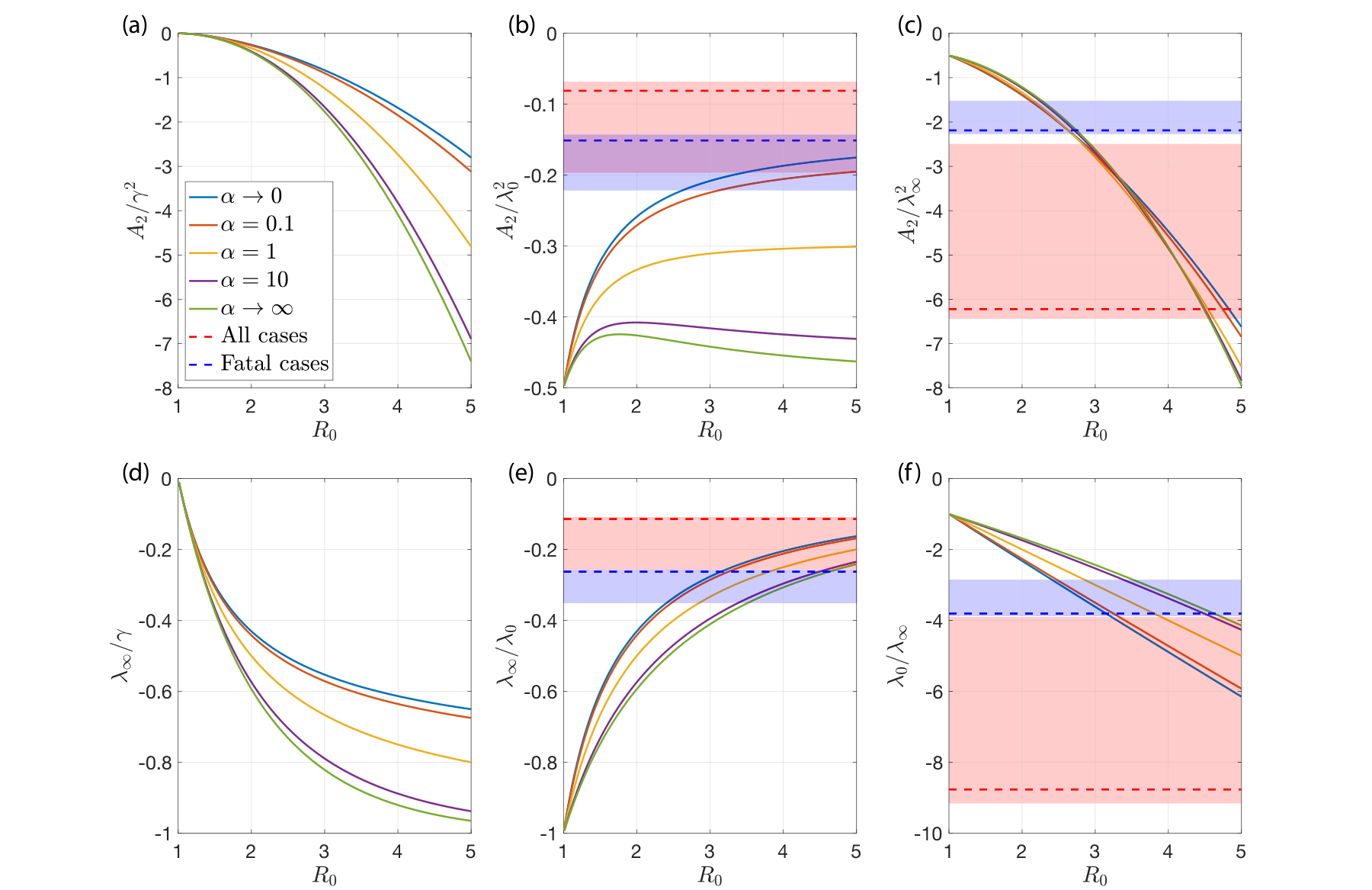
In order to understand how the shape of the wave of infections constrains the possible parameter values of $R_{0}$, $\gamma$ and $\alpha$, we consider in addition to the initial growth rate $\lambda_{0}$ and the final decay rate $\lambda_{\infty}$ two coefficients describing the epidemic dynamics near its peak, using the expansion

where the linear term disappears by definition at the maximum $J_{\rm max}=J(t_{J})$ at time $t_{J}$. The coefficients $A_{2}=\ddot{J}/J|_{t=t_{J}}$ and $A_{3}=\dddot{J}/J|_{t=t_{J}}$ can be obtained for the homogeneous and heterogeneous SIR model, see Appendix A, D and E. Fig. 5 shows dimensionless combinations of these values as a function of $R_{0}$ for different $\alpha$ ranging from the homogeneous case $\alpha\rightarrow\infty$ to strongly heterogeneous with $\alpha\rightarrow 0$ as solid lines of different color. The values obtained from the fits shown in Fig. 3 are indicated as dashed lines together with shaded regions corresponding to estimated uncertainty ranges of these values.

We find that the ratio $A_{2}/\lambda_{\infty}^{2}$, which is independent of $\gamma$ depends only weakly on $\alpha$. We can therefore use it to estimate $R_{0}$, see Fig. 5. Using $A_{2}\simeq-0.01$ day^-2 and $\lambda_{\infty}\simeq-0.07$ day^-1 determined from the data of fatal cases, we have $A_{2}/\lambda_{\infty}^{2}\simeq 2.0$ leading to the estimate $R_{0}\simeq 2.5$, see Fig. 5. This estimate can now be used to infer bounds on $\alpha$. The ratio $\lambda_{\infty}/\lambda_{0}\simeq-0.3$ is only consistent with $R_{0}\geq 2.6$ and the lower value corresponds to the limit of small $\alpha$, see Fig. 5. This reveals that $\alpha\ll 1$ must be small and that the classic SIR model with homogeneous population is not consistent with this data. We can now estimate $\gamma$ using the small $\alpha$ limit. For $R_{0}\simeq 2.6$, we have $\gamma\simeq 2\lambda_{\infty}\simeq 0.14$ day^-1, see Fig. 5 (d). The data does not provide information about the true total number of infections. Therefore the precise value of $\alpha$ remains unknown. We can use estimates from immunological studies estimating the number of infections [27, 29, 30] to determine $\alpha$. This suggests a range of about $0.01<\alpha<0.15$, corresponding to $0.65\%>f>0.04\%$. Fig. 5 also shows the estimated ranges for data on all reported cases in red. For this case the inferred values of $R_{0}$ is larger and the consistency with the data is less strong.

During an epidemic conditions can change over time. For example, mitigation by social distancing measures, quarantining or seasonal changes could affect how quickly an infection spreads on average from person to person. Given that such changes are global, they may be captured by a time-dependence of the rate $\beta(t)$[10, 12, 26]. In the following, we discuss scenarios of mitigated epidemics, starting from a reference point with an initial infection rate $\beta_{0}$ prior to mitigation. We use this reference to define the herd immunity $C_{I}$ of the population via Eq. (19). The herd immunity level depends on the basic reproduction number $R_{0}=\beta_{0}/\gamma$ and on the population heterogeneity $\alpha$. For immunity levels above herd immunity, $C\geq C_{I}$, the population is stable after mitigation measures are completely relaxed and $\beta$ is restored to its original value $\beta_{0}$.

We examine three different scenarios with a comparable total number of infections. These scenarios are shown in Fig. 6. They are characterized by different levels of immunity relative to herd immunity at July 1 and thus differ in the future behaviors beyond this time. Starting in all scenarios with $R_{0}=2$ and using $\gamma=0.24$, the model follows the initial growth at rate $\lambda_{0}$ of the reported cases. If $\beta$ is kept constant, $\beta=\beta_{0}$, the model deviates from the data at later times, see dotted lines in Fig. 6. If $\beta$ is permitted to change in time, almost any reported time course could be described by the model. We use the data to infer a time course of $\beta(t)$ such that the model follows the data, see Appendix G. The inferred values of $\beta$ are shown as circles in Fig. 6 (c), (f) and (i). In order to fit the model to the data in different mitigation scenarios, we use a piecewise linear modulation of $\beta$. The time dependence of $\beta(t)$ that resulted from these fits are shown in Fig. 6 (c), (f) and (i) as solid lines. The value of $\beta$ decreases sharply at the onset of mitigation. After this decrease it stays roughly constant or increases at constant rate, thus relaxing mitigation. The magnitude of maximal mitigation and the two slopes of $\beta(t)$ were used as fit parameters.

In the case of early mitigation, Fig. 6 (a-c), fast reduction of $\beta$ suppresses the epidemic before any appreciable progress towards herd immunity was made. Mitigation needs to be strong and sustained to be compatible with the data. By July, the population reaches only about $6-7\%$ of herd immunity in this case. Note that this is the only scenario of the classic SIR model with a homogeneous population ($\alpha\rightarrow\infty$) that could be compatible with the data.

For heterogeneous populations with $\alpha\lesssim 0.2$, scenarios with milder mitigation and with infection levels closer to herd immunity are compatible with the data, see Fig. 6 (d) and (g). A case of moderate mitigation with $\alpha=0.1$ is shown in Fig. 6 (d-f). The population in this case reaches by July 1st about $\sim 45\%$ of herd immunity. A sustained mitigation is needed to account for the data, albeit with smaller magnitude compared to the first case. If the epidemic starts slightly earlier (3 days for the case shown in Fig. 6(g-i) as compared to (d-f)), the population reaches $\sim 95\%$ of herd immunity by July 1st. Here, mitigation has the effect to reduce the cumulative number of infections as compared to a non-mitigated case ($C/N=5.8\%$ compared to $11\%$ by July 1st). This reduction of cumulative infections $C$ results from a reduction of the number of infectious individuals $I$ at the point when herd immunity is reached. In the absence of mitigation, $I$ reaches its maximum when $C=C_{I}$, whereas mitigation can reduce $I$ to small numbers as herd immunity is reached, preventing further infections. The minimal number of infections that can be achieved by temporary mitigation is $C_{I}$, which is up to $50\%$ smaller than the long lime limit $C_{\infty}$ in an unmitigated epidemic (see Fig. 2c).

The scenarios of temporary reduction of $\beta$ could capture the mitigation effects of social distancing measures. To relate the inferred time dependence of $\beta$ to measures of social activity, we show in Fig. 6(c),(f) and (i), $\beta(t)$ together with mobility data from Ref. [31] for comparison, see Appendix H. This mobility data shows a sharp decline and a slow but steady return to the initial state roughly in line with inferred changes of $\beta(t)$.

The three scenarios differ in the fraction of herd immunity they reach by July 1 and therefore in their future trajectories. However, $\beta(t)$ was adjusted by a fitting procedure such that all scenarios are consistent with the data on reported infections. This reveals that it can be difficult to distinguish effects of heterogeneity leading to a time dependent average susceptibility $\bar{x}$ from mitigation effects corresponding to time-dependent $\beta$. Indeed our analysis shows that changes in mitigation strength can be compensated to some degree by changes of heterogeneity described by $\alpha$.

References

- [1] J. D. Murray. Mathematical Biology. Interdisciplinary Applied Mathematics. Springer, New York, 3rd ed edition, 2002.
- [2] Daryl J Daley and J. M Gani. Epidemic Modelling: An Introduction. Cambridge University Press, 1999.
- [3] Herbert W. Hethcote. The Mathematics of Infectious Diseases. SIAM Review, 42(4):599–653, January 2000.
- [4] O. Diekmann, Hans Heesterbeek, and Tom Britton. Mathematical Tools for Understanding Infectious Diseases Dynamics. Princeton Series in Theoretical and Computational Biology. Princeton University Press, Princeton, 2013.
- [5] J. Brownlee. Historical note on Farr’s theory of the epidemic. BMJ, 2(2850):250–252, August 1915.
- [6] William Ogilvy Kermack and Anderson Gray McKendrick. A contribution to the mathematical theory of epidemics. Proceedings of the Royal Society of London. Series A, Containing Papers of a Mathematical and Physical Character, 115(772):700–721, August 1927.
- [7] Paul E. M. Fine. John Brownlee and the Measurement of Infectiousness: An Historical Study in Epidemic Theory. Journal of the Royal Statistical Society. Series A (General), 142(3):347, 1979.
- [8] Amit Huppert, Oren Barnea, Guy Katriel, Rami Yaari, Uri Roll, and Lewi Stone. Modeling and Statistical Analysis of the Spatio-Temporal Patterns of Seasonal Influenza in Israel. PLoS ONE, 7(10):e45107, October 2012.
- [9] Edward Goldstein, Sarah Cobey, Saki Takahashi, Joel C. Miller, and Marc Lipsitch. Predicting the Epidemic Sizes of Influenza A/H1N1, A/H3N2, and B: A Statistical Method. PLoS Medicine, 8(7):e1001051, July 2011.
- [10] Jonas Dehning, Johannes Zierenberg, F. Paul Spitzner, Michael Wibral, Joao Pinheiro Neto, Michael Wilczek, and Viola Priesemann. Inferring change points in the spread of COVID-19 reveals the effectiveness of interventions. Science, 369(6500):eabb9789, July 2020.
- [11] Rosalyn J. Moran, Erik D. Fagerholm, Maell Cullen, Jean Daunizeau, Mark P. Richardson, Steven Williams, Federico Turkheimer, Rob Leech, and Karl J. Friston. Estimating required ‘lockdown’ cycles before immunity to SARS-CoV-2: Model-based analyses of susceptible population sizes, ‘S0’, in seven European countries, including the UK and Ireland. Wellcome Open Research, 5:85, May 2020.
- [12] Seth Flaxman, Swapnil Mishra, Axel Gandy, H. Juliette T. Unwin, Thomas A. Mellan, Helen Coupland, Charles Whittaker, Harrison Zhu, Tresnia Berah, Jeffrey W. Eaton, and et al. Estimating the effects of non-pharmaceutical interventions on COVID-19 in Europe. Nature, June 2020.
- [13] Niels Becker and Paul Yip. Analysis of Variations in an Infection Rate. Australian Journal of Statistics, 31(1):42–52, March 1989.
- [14] Herbert W. Hethcote. An immunization model for a heterogeneous population. Theoretical Population Biology, 14(3):338–349, December 1978.
- [15] M. Gabriela M. Gomes, Rodrigo M. Corder, Jessica G. King, Kate E. Langwig, Caetano Souto-Maior, Jorge Carneiro, Guilherme Goncalves, Carlos Penha-Goncalves, Marcelo U. Ferreira, and Ricardo Aguas. Individual variation in susceptibility or exposure to SARS-CoV-2 lowers the herd immunity threshold. medRxiv, page 2020.04.27.20081893v3, May 2020.
- [16] J. O. Lloyd-Smith, S. J. Schreiber, P. E. Kopp, and W. M. Getz. Superspreading and the effect of individual variation on disease emergence. Nature, 438(7066):355–359, November 2005.
- [17] O. Diekmann, J.A.P. Heesterbeek, and J.A.J. Metz. On the definition and the computation of the basic reproduction ratio R 0 in models for infectious diseases in heterogeneous populations. Journal of Mathematical Biology, 28(4), June 1990.
- [18] Tom Britton, Frank Ball, and Pieter Trapman. A mathematical model reveals the influence of population heterogeneity on herd immunity to SARS-CoV-2. Science, page eabc6810, June 2020.
- [19] Per Bak, Chao Tang, and Kurt Wiesenfeld. Self-organized criticality: An explanation of the 1/ f noise. Physical Review Letters, 59(4):381–384, July 1987.
- [20] Michael F. Shlesinger. Fractal Time and 1/f Noise in Complex Systems. Annals of the New York Academy of Sciences, 504(1 Perspectives):214–228, July 1987.
- [21] Luís A. Nunes Amaral, Sergey V. Buldyrev, Shlomo Havlin, Michael A. Salinger, and H. Eugene Stanley. Power Law Scaling for a System of Interacting Units with Complex Internal Structure. Physical Review Letters, 80(7):1385–1388, February 1998.
- [22] Didier Sornette. Probability Distributions in Complex Systems. In Robert A. Meyers, editor, Encyclopedia of Complexity and Systems Science, pages 7009–7024. Springer New York, New York, NY, 2009.
- [23] Rudragouda Channappanavar, Jincun Zhao, and Stanley Perlman. T cell-mediated immune response to respiratory coronaviruses. Immunologic Research, 59(1-3):118–128, August 2014.
- [24] Julian Braun, Lucie Loyal, Marco Frentsch, Daniel Wendisch, Philipp Georg, Florian Kurth, Stefan Hippenstiel, Manuela Dingeldey, Beate Kruse, Florent Fauchere, and et al. SARS-CoV-2-reactive T cells in healthy donors and patients with COVID-19. Nature, July 2020.
- [25] Robert-Koch-Institut. Fallzahlen in Deutschland. https://npgeo-corona-npgeo-de.hub.arcgis.com/ Accessed: 16 July 2020. dl-de/by-2-0 (www.govdata.de/dl-de/by-2-0).
- [26] Stephen M. Kissler, Christine Tedijanto, Edward Goldstein, Yonatan H. Grad, and Marc Lipsitch. Projecting the transmission dynamics of SARS-CoV-2 through the postpandemic period. Science, 368(6493):860–868, May 2020.
- [27] Hendrik Streeck, Bianca Schulte, Beate Kuemmerer, Enrico Richter, Tobias Hoeller, Christine Fuhrmann, Eva Bartok, Ramona Dolscheid, Moritz Berger, Lukas Wessendorf, and et al. Infection fatality rate of SARS-CoV-2 infection in a German community with a super-spreading event. medRxiv, page 2020.05.04.20090076, May 2020.
- [28] John P. A. Ioannidis, Cathrine Axfors, and Despina G. Contopoulos-Ioannidis. Population-level COVID-19 mortality risk for non-elderly individuals overall and for non-elderly individuals without underlying diseases in pandemic epicenters. medRxiv, page 2020.04.05.20054361, April 2020.
- [29] John P. A. Ioannidis. The infection fatality rate of COVID-19 inferred from seroprevalence data. medRxiv, page 2020.05.13.20101253, May 2020.
- [30] Marina Pollán, Beatriz Pérez-Gómez, Roberto Pastor-Barriuso, Jesús Oteo, Miguel A Hernán, Mayte Pérez-Olmeda, Jose L Sanmartín, Aurora Fernández-García, Israel Cruz, Nerea Fernández de Larrea, and et al. Prevalence of SARS-CoV-2 in Spain (ENE-COVID): A nationwide, population-based seroepidemiological study. The Lancet, July 2020.
- [31] Google LLC. Google covid-19 community mobility reports. https://www.google.com/covid19/mobility/ Accessed: 13 July 2020.
- [32] N Ferguson, D Laydon, G Nedjati Gilani, N Imai, K Ainslie, M Baguelin, S Bhatia, A Boonyasiri, ZULMA Cucunuba Perez, G Cuomo-Dannenburg, and et al. Report 9: Impact of non-pharmaceutical interventions (NPIs) to reduce COVID19 mortality and healthcare demand. Technical report, Imperial College London, March 2020.