Multiobjective Backstepping Controller for Parallel Buck Converter

The control objectives for this system are achieved by using separate backstepping-based controller for each converter. The first converter ensures that the output voltage of converter 1 traces the given reference voltage, $V_{ref}$. The second converter adjusts its current such that the load sharing is proportional.

From equations  (1) and  (3), state space equation for Converter 1 is

where $C=C_{1}+C_{2}$. Let $e=V_{ref}-V_{o}$, the error between the desired and actual output voltage. Taking the derivative, we get

In equation  (5), $i_{L_{1}}$ acts as the virtual control variable. Therefore, adding and subtracting $i_{L_{1D}}$, which is the desired value for $i_{L_{1}}$ we get

where, $\tilde{i}_{L_{1}}=i_{L_{1D}}-i_{L_{1}}$. If $i_{L_{1D}}=\frac{V_{ref}}{R}-\frac{i_{L_{2}}}{R}+k_{1}e$, where $k1>0$, the error dynamics becomes

which is a stable system. The variable $k_{1}$ is added to ensure faster response.

In order to select the appropriate duty cycle $d_{1}$, let $\dot{i}_{L_{1}}=W_{1}$. Consider the Lyapunov Function candidate (LFC)

For the Lyapunov function to be negative definite, select

Substituting $W_{1}$ in Lyapunov function expression gives

Since $\dot{V}_{1}$ is negative definite, error $e\rightarrow 0$ and $\tilde{i}_{L_{1}}\rightarrow 0$ Therefore, the duty cycle for the first converter for successful voltage tracking is

The current sharing is ensured by a separate backstepping controller which controls Converter 2. For proportional current sharing between the two converters, say the maximum current that can be supplied by the two converters be $I_{1m}$ and $I_{2m}$. Then the goal of the second controller is to ensure $\left(i_{L_{1}}/I_{1m}-i_{L_{2}}/I_{2m}\right)\rightarrow 0$. The state space equation for Converter 2 is as follows

Let $e_{2}=i_{L_{1}}/I_{1m}-i_{L_{2}}/I_{2m}$, then the error dynamics for the second controller can be written as

Let $\left(\frac{1}{I_{2m}L_{2}}-\frac{1}{I_{1m}L_{1}}\right)=X$, then equation  (13) becomes

where, $V_{oD}$ is the desired output voltage and $\tilde{V}_{o}=V_{oD}-V_{o}$. If $V_{oD}=\frac{1}{X}\left(-\frac{d_{1}V_{1}}{I_{1m}L_{1}}+\frac{d_{2}V_{2}}{I_{2m}L_{2}}-k_{2}e_{2}\right)$, where $k_{2}>0$, then the error dynamics becomes a stable system as shown below

To check the stability of the system, consider the Lyapunov Function candidate

Let $W_{2}=\dot{i}_{L_{2}}$ and differentiate the LFC, which gives

Note that in equation  (17), since the controller is designed considering converter 2, the duty cycle for converter 1, $d_{1}$, is treated constant. For equation  (17) to be negative definite, select

Since $W_{2}=\dot{i}_{L_{2}}$, using equations  (18) and  (12) we get

The designed controller is first tested on a constant resistor load. The system parameters for each converter is given in Table I. The two converters are similar but the maximum current capacity of converter 1 is 5 A while that of converter 2 is 2 A. The parallel converters are supplying current to a 10 $\Omega$ resistor. The goal is to ensure that the per unit current supplied by each converter is equal and the output voltage is regulated at a given $V_{ref}$. Herein, $V_{ref}=8$, $k_{1}=k_{2}=1$.

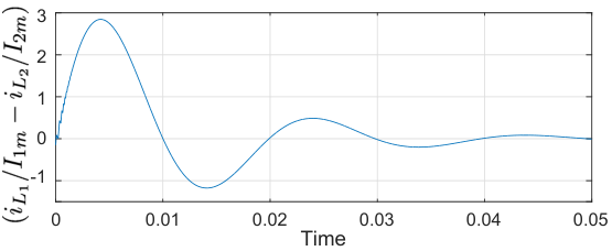
Figure 3 shows the variation of output voltage. It can be seen that the controller matches the output voltage to the desired voltage. Figure 4 shows the plot for the difference between the per unit current supplied by both the sources. It can be observed that the controller ensures that the per unit current supplied by each converter is same.

In this section, performance of the controller is evaluated when there is a sudden change in load. For this simulation, the resistance of the load is suddenly changed from 10 $\Omega$ to 15 $\Omega$ at time $t=0.05$ seconds. Figures 5 and 6 show the variation of output voltages and the difference between the per unit currents. It can be seen that controller quickly regulates the output voltage and balances the current sharing.

References

- [1] J. M. Guerrero, J. C. Vasquez, J. Matas, L. G. de Vicuna, and M. Castilla, “Hierarchical control of droop-controlled ac and dc microgrids—a general approach toward standardization,” IEEE Trans. Ind. Electron., vol. 58, no. 1, pp. 158–172, Jan. 2011.
- [2] T. Dragicevic, X. Lu, J. C. Vasquez, and J. M. Guerrero, “Dc microgrids—part i: A review of control strategies and stabilization techniques,” IEEE Trans. Power Electron., vol. 31, no. 7, pp. 4876–4891, Jul. 2016.
- [3] P. J. Grbovic, “Master/slave control of input-series- and output-parallel-connected converters: Concept for low-cost high-voltage auxiliary power supplies,” IEEE Trans. Power Electron., vol. 24, no. 2, pp. 316–328, Feb. 2009.
- [4] R. Giri, V. Choudhary, R. Ayyanar, and N. Mohan, “Common-duty-ratio control of input-series connected modular dc-dc converters with active input voltage and load-current sharing,” IEEE Trans. Ind. Appl., vol. 42, no. 4, pp. 1101–1111, Jul. 2006.
- [5] S. Moayedi, V. Nasirian, F. L. Lewis, and A. Davoudi, “Team-oriented load sharing in parallel dc–dc converters,” IEEE Trans. Ind. Appl., vol. 51, no. 1, pp. 479–490, Jan. 2015.
- [6] V. Nasirian, A. Davoudi, and F. L. Lewis, “Distributed adaptive droop control for dc microgrids,” in Proc. 29th IEEE Appl. Power Electron. Conf. Expo., 2014, pp. 1147–1152.
- [7] R. W. Erickson and D. Maksimovic, Fundament of Power Electronics, 2nd ed. New York, USA: Kluver Academic Publishers, 2001.
- [8] J. Mahdavi, A. Emaadi, M. D. Bellar, and M. Ehsani, “Analysis of power electronic converters using the generalized state-space averaging approach,” IEEE Trans. Circuits Syst. I: Fundam. Theory Appl., vol. 44, no. 8, pp. 767–770, Aug 1997.