Inverse Mixed Integer Optimization:
Polyhedral Insights and Trust Region Methods
Abstract
Inverse optimization – determining parameters of an optimization problem that render a given solution optimal – has received increasing attention in recent years. While significant inverse optimization literature exists for convex optimization problems, there have been few advances for discrete problems, despite the ubiquity of applications that fundamentally rely on discrete decision-making. In this paper, we present a new set of theoretical insights and algorithms for the general class of inverse mixed integer linear optimization problems. Specifically, a general characterization of optimality conditions is established and leveraged to design new cutting plane solution algorithms. Through an extensive set of computational experiments, we show that our methods provide substantial improvements over existing methods in solving the largest and most difficult instances to date.
keywords
Inverse Optimization, Mixed Integer Programming, Cutting Planes, Inverse-Feasibility, Decomposition Methods, Trust Regions1 Introduction
Inverse optimization – inferring unobserved parameters of a (forward) optimization problem that render a given (forward-feasible) solution optimal – has received increasing attention in recent years. Most of the literature has focused on inverse optimization for convex forward optimization problems, allowing the bi-level inverse problem to be reformulated as a single-level convex problem using the Karush-Kuhn-Tucker conditions. Examples include linear (Zhang and Liu 1996, Ahuja and Orlin 2001, e.g.,), multiobjective linear (Naghavi et al. 2019, e.g.), conic (Iyengar and Kang 2005, e.g.) and general convex optimization problems (Zhang and Xu 2010, Zhang et al. 2010, e.g.). These models have been applied across a wide range of application domains (see Section 1.1.2) and have also been extended methodologically in several modern directions including estimating model parameters from multiple observed solutions while considering concepts such as statistical consistency (Aswani et al. 2018) or distributional robustness (Esfahani et al. 2018).
In contrast, there have been very few advances in inverse optimization for discrete forward problems, despite the ubiquity of methodological research in discrete optimization and real-world applications that have discrete decisions. Part of the challenge may stem from the fact that the optimality conditions for discrete problems like mixed integer linear optimization (MILO) generally do not lead to computationally tractable solution algorithms like they do for convex problems. For example, Schaefer 2009 and Lamperski and Schaefer 2015 demonstrate how superadditive duality can be used to develop exact reformulations of bi-level inverse integer and mixed-integer optimization problems, respectively. However, the resulting single-level formulation is an exponentially large linear program that is intractable beyond problems with few variables.
The other main idea in the literature for a general-purpose inverse MILO solution method is a cutting plane algorithm. First proposed in Wang 2009, the idea is to decompose the inverse MILO problem into a master problem and a subproblem. The former is a relaxation of the inverse MILO problem that provides candidates for parameters to be inferred, whereas the latter identifies extreme points of the convex hull of the forward-feasible region that generate cuts to send back to the master problem. While it was shown that small problems could be solved efficiently, this approach does not scale well to larger problems. The computational cost of computing each extreme point is large in general, since it involves solving an instance of the forward MILO problem. The only advance to this method since its development was a proposed heuristic that parallelizes the computation of extreme points (Duan and Wang 2011).
In this paper, we develop a new cutting plane framework for solving inverse MILO problems. We begin by providing a more general characterization of the optimality conditions of the inverse MILO problem relative to previous literature. We demonstrate that extreme points are sufficient but not necessary for characterizing inverse optimality, and that more parsimonious representations of the problem exist. Using this insight, we develop a new cutting plane method where the cut generation subroutine efficiently identifies interior forward-feasible points using trust regions. These cuts come at significantly lower computational cost compared to cuts generated from extreme points. In addition, we observe that inverse MILO problems can be solved with many fewer cuts compared to the classical cutting plane algorithm.
Our specific contributions are:
- 1.
We present a novel characterization of optimality conditions for inverse MILO problems by introducing the concept of generator sets (Section 2). Generator sets characterize the complete family of reformulations of the MILO problem that preserve the feasible region of the inverse optimization problem. Our main result provides necessary and sufficient conditions for any set to be a generator set. We also show that there exist “small” generator sets, which are attractive from a computational perspective.
- 2.
Motivated by our theoretical insights, we propose a new family of cutting plane methods that restrict the feasible region of the MILO problem using trust regions (Section 3). We also propose computational enhancements that further speed up the algorithm (Section 4). Our algorithms generalize the classical cutting plane approach to solving inverse MILO problems.
- 3.
We propose an extension of the inverse MILO problem to a setting with multiple input data points and illustrate how our cutting plane algorithm can be easily extended to solve this problem (Section 5).
- 4.
Through a comprehensive numerical study over instances drawn from the MIPLIB 2017 benchmark library (Gleixner et al. 2019), we demonstrate that our new cutting plane algorithm significantly outperforms the state-of-the-art algorithm by solving the largest and most difficult problem instances in the literature to date (Sections 6 and 7). We observe that our new cut generation methods can both substantially speed up cut generation and reduce the number of cuts required.
1.1 Related literature
Below, we review relevant inverse optimization models and solution methods, as well as the main application areas in which these models can be found.
1.1.1 Models and methods.
The classical inverse optimization problem, which is to infer a set of model parameters that render a given feasible solution optimal, has been studied over a wide range of problem settings. The parameters that are inferred can be the cost vector or the constraints. While there are a few studies that focus on estimating constraint parameters (Güler and Hamacher 2010, Birge et al. 2017, Chan and Kaw 2020), the vast majority of papers focus on estimating the cost vector. Most early works focused on deriving algorithms to solve inverse models for particular forward problems (e.g., shortest path, minimum spanning tree), while more recent works consider general-purpose methods for broader classes of forward problems (e.g., mixed integer optimization). Heuberger 2004 provides an overview of the early works whereas the literature discussed in the introduction are examples of more recent works. In this paper, we focus on estimating the cost vector for general mixed integer forward problems, particularly in the form of the classical inverse model.
Inverse optimization problems with “noisy” data have also been studied (Troutt et al. 2006, Keshavarz et al. 2011, Chan et al. 2014, Chan et al. 2019, e.g.). These problems are characterized by the fact that there does not exist a set of (non-trivial) parameters that render a given solution, or a set of solutions, optimal. For these problems, the cost vector is estimated by minimizing various notions of suboptimality (Bertsimas et al. 2015, Aswani et al. 2018, Esfahani et al. 2018, Babier et al. 2021, e.g.). Although we focus predominantly on the classical inverse model in the paper, we show that the insights and methods developed can be easily extended to a model for multiple “noisy” data points that resembles the models found for inverse convex optimization.
Finally, we borrow the term “trust region” from the general optimization community, a term which broadly describes the restriction of a particular search space. The use of trust region concepts have appeared in a range of different domains such as nonlinear optimization and, more relevant to our paper, decomposition algorithms. Within the latter domain, trust regions have been applied to the master problems of decomposition models for stochastic programming, and are shown to help generate stronger cuts in this context (Linderoth and Wright 2003, Zverovich et al. 2012, Rahmaniani et al. 2017). In contrast, we apply trust regions to the cut generation problem in our decomposition framework, which leads to improvements in both strength of cuts and cut generation time over a wide array of problem structures.
1.1.2 Applications.
Inverse optimization has been studied in a wide variety of applications to estimate latent parameters and infer subjective preferences using observed decision data. Examples of such applications can be found in energy markets (Ruiz et al. 2013, Saez-Gallego et al. 2016, Birge et al. 2017), healthcare (Erkin et al. 2010, Chan et al. 2014, Babier et al. 2020), finance (Bertsimas et al. 2012, Utz et al. 2014, Yu et al. 2020), and transportation (Chow and Recker 2012, Chow et al. 2014, Xu et al. 2018, Zhang et al. 2018), where inverse optimization is used to provide insights into market structure, treatment design, risk aversion and route-choice preferences, respectively. This literature makes use of both classical inverse models and inverse models for “noisy” decision data.
Inverse optimization is also prevalent in the bi-level optimization literature, especially in regards to pricing and incentive design problems. Recent examples of such applications include the design of tolls in traffic and commodity transportation networks (Marcotte et al. 2009, Brotcorne et al. 2011, Esfandeh et al. 2016, Kuiteing et al. 2017, Kuiteing et al. 2018), price schedules and carbon taxes in energy systems (Zhou et al. 2011, Afşar et al. 2021), and profit-sharing mechanisms in carrier alliances (Agarwal and Ergun 2010, Houghtalen et al. 2011). Here, the classical inverse optimization model appears as a “subproblem” within the solution process used to solve these pricing problems. Specifically, a “master problem” generates a decision “target” (e.g., a sustainable routing decision) while an inverse model computes a set of objective perturbations (e.g., tolls on roads) for which the target becomes an optimal decision for an underlying decision-maker (e.g., a transportation company). The master problem can also propose new targets if the inverse subproblem is infeasible (Afşar et al. 2021).
Despite the ubiquity of decision-making models in these application areas that fundamentally rely on making discrete choices, existing literature has focused primarily on inverse optimization for continuous forward problems. The few exceptions to date are in energy planning (Zhou et al. 2011), transportation (Chow and Recker 2012), and sustainability (Turner and Chan 2013). The first two applications were formulated as general inverse MILO problems and applied the classical cutting plane algorithm (Wang 2009). The sustainability application, an inverse knapsack problem, was reformulated using superadditive duality and solved by restricting focus to linear functions.
1.2 Notation
Throughout the paper, vectors and matrices are written in bold, while sets are defined using calligraphic letters. Subscripts denote specific elements of a vector, whereas superscripts denote different vectors. We use to denote the transpose operator. For any set , is its convex hull, is its set of extreme points, and .
2 Structure of Inverse MILO Problems
In this section, we study the structure of inverse MILO problems. We provide a novel characterization of inverse-feasibility over general non-convex forward optimization problems. We do this through the definition of a generator set, which characterizes the complete family of reformulations of the forward optimization problem that preserve the feasible region of the inverse optimization problem. In turn, we show how certain feasible region definitions are amenable to more efficient solution methods for the inverse optimization problem. Proofs of our results are provided in the Appendix.
2.1 Problem definition
Our inverse optimization model is based on the following MILO problem, known as the forward problem:
| (1) | ||||
Let be the optimal solution set of . Elements of and are called forward-feasible and forward-optimal, respectively. For a given forward-feasible solution , let define the inverse-feasible region, which is the set of all cost vectors that render the solution optimal, i.e.,
| (2) |
The inverse optimization problem is defined as the following optimization model,
| (3) | ||||
which seeks to find a cost vector that minimizes an objective function , is inverse-feasible, and satisfies any context-specific constraints . A common choice of is
The inverse optimization model with this objective seeks to find feasible cost vectors that minimize the deviation to a given reference cost vector , as measured by the Manhattan distance. Practically, this objective function is relevant in many applications (see Section 1.1 for details). First, in estimation problems, can represent an initial estimate of the cost vector, and given an observed decision , the cost estimates can be refined (minimally) to be compatible with . For example, may represent an estimate of network link costs used to describe route preferences (e.g., where initial estimates are based on road distances), and an observed routing decision can be used to refine these estimates (Burton and Toint 1992, Ahuja and Orlin 2001, Chen et al. 2021). Second, in bi-level optimization problems, represents the known cost vector of a decision-maker, and a set of objective perturbations to can be designed and prescribed such that a decision target becomes an optimal choice for the decision-maker. For example, the elements of may represent the cost of producing energy using different resources, in which case the vector would describe the value of carbon taxes or subsidies that must be imposed on each resource for a low-emission production plan to become optimal for an energy producer (Zhou et al. 2011, Rathore and Jakhar 2021). In these settings, there may be context-specific constraints on , such as non-negativity (), integrality (), variable bounds (), or a transformation into a multi-objective problem ( where are given objectives and is a decision vector of objective weights).
From this point on, we present our inverse optimization model as
| (4) | ||||
We make this modeling choice because the model is well-motivated and because it is the formulation that is studied in all previous works on inverse mixed integer optimization (Wang 2009, Schaefer 2009, Duan and Wang 2011, Lamperski and Schaefer 2015, Bulut and Ralphs 2015). Nonetheless, we emphasize that this modeling choice comes without loss of generality. The theoretical insights and methodological contributions presented in this paper focus exclusively on difficulties posed by the inverse-feasibility constraint (equation (2)), and are thus directly applicable for any inverse MILO problem in the form of model (3). We also assume without loss of generality that the inverse optimization problem is feasible. If it is not, then the methods proposed in this paper can prove its infeasibility.
In the remainder of this section (Sections 2.2 and 2.3), we focus on the core difficulty of solving the inverse MILO problem: characterizing the inverse-feasible region . In contrast to convex optimization problems, where this condition can be transformed into convex constraints using the Karush-Kuhn-Tucker conditions, determining whether a given is optimal with respect to some , let alone the that optimizes the objective function of the inverse problem, requires solving the forward MILO problem, which is NP-hard in general. Furthermore, attempting to use inverse linear optimization models to approximate inverse MILO models by ignoring the integrality constraints of the forward-feasible region can result in arbitrarily bad approximations. This is further discussed and illustrated in Section B of the Electronic Companion.
2.2 Preliminary remarks
We first note three basic properties of the inverse-feasible region, then describe it using a set of linear constraints.
Remark 2.1
The inverse-feasible region is nonempty, since .
Remark 2.2
The inverse-feasible region contains only the zero vector, i.e., , if and only if is full dimensional and is not on the boundary of conv(). If there exists at least one equality constraint or one binary variable used in the description of , then for all . Similarly, if there exists at least one constraint that is binding at , including variable bounds, then .
Remark 2.3
While the forward-feasible region does not have to be bounded, the inverse-feasible region will only contain objective vectors for which the forward problem is bounded. In particular, if is a nonzero vector in the recession cone of , then we have . The reason is that is assumed to be forward-optimal with a finite objective value (under an unobserved objective function) and . Thus . In other words, no such can make forward-optimal.
A natural way to explicitly formulate model (4) is to re-write using a potentially infinite set of linear constraints
| (5) |
suggesting that a cutting plane method can be used to solve . Indeed, Wang 2009 proposed a simple cutting plane algorithm to solve the inverse MILO problem in a finite (but exponential, in general) number of iterations by noting that it is sufficient to replace in equation (5) with the extreme points of its convex hull.
The cutting plane algorithm proposed in Wang 2009 starts without constraints (6b), and iteratively adds cuts of this form through the computation of new extreme points . The efficiency of this approach depends heavily on the difficulty of generating cuts, which amounts to solving the forward MILO problem, as well as the number of extreme points of the convex hull of (Bulut and Ralphs 2015). With the exception of parallelizing the search for extreme points (Duan and Wang 2011), the algorithm proposed in Wang 2009 remains the state-of-the-art in solving inverse MILO problems.
2.3 Optimality conditions
The main insight from Wang 2009 is that replacing constraints (5) with (6b) preserves the set of optimal solutions to the inverse optimization problem, i.e., . In this subsection, we characterize the full family of sets such that .
Definition 2.5
Given , any set for which
| (7) |
is a generator set for . If , then is a forward-feasible generator set.
Examples of generator sets include and , with the latter being a forward-feasible generator set.
Next, we demonstrate there may exist a large family of such sets for . First, note that constraint set (5) defines a polyhedral cone. Second, each half-space induced by a feasible point is not uniquely determined by , but rather by any multiple of the vector . In other words, the half-space induced by is the same as the one induced by for any . The same cut can thus be induced by infinitely many other points of .
These observations are illustrated in Figure 1. The extreme points in Figure 1(a) induce half spaces for and the intersection of these half-spaces is the cone shown in Figure 1(b). However, the same cone can be formed using the (blue) diamond points, all of which are interior forward-feasible points, plus , in Figure 1(a).
The last observation above is formalized in the following lemma. Let , , define a point along the ray from to .
Lemma 2.6
Let and for arbitrary positive scalars . Then,
Lemma 2.6 shows that the set of extreme points is not necessary to characterize and can instead be replaced with a set of interior and/or exterior points. This observation can be generalized with a necessary and sufficient condition for any collection of points to be a generator set. Let denote the polyhedral cone pointed at generated by .
Theorem 2.7
A set is a generator set if and only if .
While Lemma 2.6 shows that generator sets can be constructed without using any extreme points, Theorem 2.7 goes further and shows that far fewer points than the number of extreme points may be sufficient to construct a generator set. As long as the set of extreme rays of are the same as those of , then is a generator set – all other points in that do not form an extreme ray are redundant in defining the inverse-feasible region. Referring back to Figure 1(a), this result implies that any two points and with are sufficient to define the generator set in that example. In Figure 1(b), the inverse-feasible region is exactly the intersection of the half-spaces determined by and .
Note that for any forward-feasible point , the ray is in . Thus, for any collection of forward-feasible points . Then, the set is a forward-feasible generator set if , or equivalently if . This is shown by the following corollary.
Corollary 2.8
A set is a forward-feasible generator set if and only if .
Analyzing forward-feasible generator sets can be particularly informative for the design of cutting plane algorithms. For example, inverse MILO problems can be solved by the cutting plane algorithm presented in Wang 2009 because is a forward-feasible generator set. Below, we present an equivalent characterization of forward-feasible generator sets that does not rely on the notion of rays. This result provides useful intuition to aid in designing a new cutting plane algorithm. Let denote a closed ball of radius around .
Theorem 2.9
A set is a forward-feasible generator set if and only if and there exists an such that
| (8) |
Theorem 2.9 states that a set is a forward-feasible generator set if and only if the convex hull of the set of points in and contains an epsilon ball around intersected with the convex hull of . Going back to Figure 1(a), is a forward-feasible generator set since the convex hull of contains the part of an epsilon ball around inside , which is shaded in red. Considering the ray , only is a forward-feasible point, which means that any forward-feasible generator set must include . However, there are multiple forward-feasible points along the ray , which means that any of those feasible points, namely (5,10), (6,10) or (7,10), can be part of the forward-feasible generator set.
The two key takeaways from Theorem 2.9 are that a forward-feasible generator set can: (i) consist of many fewer than points, and (ii) be generated from non-extreme points that lie much closer to .
3 Cutting Plane Algorithm with Trust Regions
The theoretical insights from the previous section indicate that a new approach to generating cuts may yield a more effective solution algorithm. Instead of generating cuts by identifying extreme points of the convex hull of the forward-feasible region , we generate cuts by identifying interior points of , which we accomplish using trust regions. More specifically, we intersect with a trust region, and generate cuts at interior points of obtained as extreme points of the convex hull of this restriction of .
Let be a trust region around the point of size , defined as
| (9) |
We simplify notation to when the parameter is not the focus of discussion.
Guided by Theorem 2.9, we define trust regions to be centered at . The trust region, when imposed onto , represents an attempt to capture a forward-feasible generator set. The 1-norm in equation (9) is chosen because the trust region has a polynomial number of extreme points. When intersected with , the resulting restricted forward-feasible region itself is more likely to have a smaller number of extreme points compared to . This can reduce the number of forward-feasible points that need to be identified in order to build a generator set. Furthermore, the extreme points of this smaller, restricted region may also be computationally easier to identify. These considerations will be discussed in detail below.
3.1 Model decomposition and cutting plane framework
The inverse MILO problem is decomposed into a master problem, describing a relaxation of the inverse model (4), and a cut generation subroutine that is used to iteratively tighten the master problem. The framework of our cutting plane algorithm is given in Algorithm 1. A global information set is used to pass information between successive iterations of the subroutine, which specifically includes the trust region and outer-loop index for our purposes. It is initialized with a trust region of size centered at , and the iteration index .
Input: An inverse MILO problem instance , initial trust region size
Output: An inverse-optimal solution
The master problem is defined below, where denotes a finite set of forward-feasible points.
| (10a) | ||||
| subject to | (10b) | |||
| (10c) | ||||
| (10d) | ||||
Constraints (10b) ensure that is optimal with respect to over . As mentioned in Remark 2.3, the inverse-feasible region only contains cost vectors for which the forward optimization problem is bounded. However, due to its relaxed nature, the master problem can propose cost vectors that lead to unbounded forward problems in the subroutine. This can be prevented by constraints (10c) and (10d), as proposed in Wang 2009, which are not needed if the forward-feasible region is bounded. Let denote an optimal solution to the master problem .
3.2 Cut generation subroutine
Given , the cut generation subroutine either finds a feasible point satisfying (i.e., ), which generates a cut, or returns , verifying that . Note that the verification in the latter case requires solving the forward problem , which means the cut generation subroutine is at least as hard.
The cut generation subroutine is presented in Subroutine 1. It consists of four key components: the cut generation problem (Step 3) and three functions to modify the trust region (Steps 2, 5 and 8), which we describe next.
Input: A candidate objective , forward-feasible point , forward-feasible region , information set
Output: A forward-feasible point and updated information set
3.2.1 Cut generation problem (Step 3).
Given a candidate objective and a trust region , the cut generation problem is the forward problem solved over (i.e., ), which we refer to as a subregion of . We note that the choice of 1-norm in the definition of employed trust regions ensures that the cut generation problem remains linear.
If the optimal solution of the cut generation problem satisfies the condition , then is returned; we call such an a violated forward-feasible point. If no cut is found, then there are two possibilities depending on whether a trust region was used. If no trust region was used, i.e., , then is returned and Algorithm 1 terminates with . Otherwise, renders optimal over a subregion of , but not necessarily over . Thus, larger subregions need to be considered before it can be verified that no additional violated cuts exist, which leads to a trust region update.
3.2.2 UPDATE function (Step 8).
When a subregion has been exhausted of violated cuts, we increase the size of the trust region to for some :
| (11) |
For example, setting doubles the size of the trust region each time UPDATE is called. There is a natural trade-off to be considered when choosing . If is too small, then the trust regions grow slowly and may lead to the generation of subregions with no violated cuts. This will result in time-consuming, “empty” calls to the cut generation problem, i.e., calls in which the cut generation problem is solved but is unable to generate any violated forward-feasible point. On the other hand, if is too large, the computational advantages of solving the cut generation problem over a smaller subregion with fewer extreme points may quickly be lost.
3.2.3 REMOVE function (Step 2).
The REMOVE function periodically removes the existing trust region (by setting ) at regular intervals in both outer (i.e., master) iterations and inner (i.e., subroutine) iterations . In particular, for fixed index values and ,
| (12) |
In other words, the cut generation problem is solved over every iterations in the outer loop and when the inner loop reaches the iteration limit of . The REMOVE function guarantees finite convergence of Algorithm 1, irrespective of how the UPDATE function is defined, because an extreme point of is returned at least every iterations in a finite number of (at most ) attempts to verify that a candidate objective is inverse-feasible when no more violated cuts exist.
Note that the classical cutting plane algorithm proposed in Wang 2009 is a special case of our trust region-based approach where .
3.2.4 SAVE function (Step 5).
The SAVE function is called when a forward-feasible point yielding a violated cut is found by the cut generation problem. If such a point is found during an iteration where the trust region is (i.e., when REMOVE is called), the SAVE function saves the previous trust region. On the other hand, if the REMOVE function did not remove the trust region during the current iteration, then the current trust region is saved. This ensures that there always exists a “non-trivial” trust region () saved.
Mathematically, the SAVE function is defined as:
3.2.5 Discussion and example.
Trust regions can reduce the difficulty of solving the cut generation problem by reducing the size of the forward-feasible region. However, they can also lead to the generation of stronger cuts.
We use Figure 2(a) to illustrate this latter point. A trust region of size one () is imposed on a two-dimensional integer forward-feasible region, creating a subregion containing two extreme points (indicated using blue diamonds), excluding . Those two extreme points of the subregion have the same cut generation potential as the five extreme points of labeled in gray. More specifically, the set of cuts generated by the former set of extreme points can dominate those generated by the latter. Once this trust region is exhausted, it must be updated.
In Figure 2(a), increasing the size of the trust region by a single unit would cover , the only additional point needed to build a generator set. The trust region approach guarantees that at most three cuts need to be generated, or equivalently three forward-feasible points need to be identified, to solve the inverse MILO problem. On the other hand, the cutting plane algorithm without trust regions, which computes extreme points of , may require generating many more cuts.
The REMOVE function periodically removes trust regions and provides opportunities for the algorithm to compute points outside of the existing trust region. We consider another example in Figure 2(b) with a trust region of over a different two-dimensional integer forward-feasible region. Assuming the subregion has been exhausted of cuts, removal of this trust region would lead to the computation of with certainty, as it is the only extreme point of that can still generate a valid cut. This would terminate the algorithm at the next step. On the other hand, if the size of the trust region was increased incrementally each time without removing the trust region, many unnecessary interior points would be computed before a sufficiently large trust region captures . Periodic removal of trust regions thus helps to reduce the potential of being overly-conservative, and when used in conjunction with trust regions create an effective cut generation subroutine.
4 Algorithm Enhancements
In this section, we propose two enhancements to Subroutine 1 that can be implemented independently or together. These two enhancements are introduced to improve cut generation speed, particularly during iterations when the subregion is large.
4.1 Early-stop heuristic for the cut generation problem
As defined in Subroutine 1, the cut generation problem is solved to optimality in each iteration. However, this can be time consuming, particularly during iterations where the trust region is large or removed entirely. Here, we introduce a solution time threshold . If the cut generation problem is not solved by , but at least one violated forward-feasible point has been found, the feasible point of maximum violation is returned. If no violated forward-feasible point has been found by , the cut generation problem will return the first such point found after . This enhancement can reduce the cut generation time and can be effective for two reasons: (i) Solving the cut generation problem may not necessarily provide the best cuts anyways, as discussed in Section 2, and (ii) the solver may have already found an optimal violated forward-feasible point in the cut generation problem but has not computed a bound strong enough to prove its optimality. When a standard MILO solver, such as CPLEX and Gurobi, is used to solve the forward problem in Subroutine 1, the early-stop heuristic can be implemented using a callback function.
4.2 Stochastic dimensionality reduction of the trust region
This enhancement is motivated by the observation that a violated forward-feasible point generated within a trust region may have many components with the same value as the corresponding components in . For example, if contains only integer variables, then all forward-feasible points within a trust region around will differ from by at most components. By explicitly restricting which subset of components can differ from the values of , we can decrease the dimensionality and hence the size of the cut generation problem.
Let and
| (13) |
define a lower dimensional trust region containing points that can differ from only in the indices contained in .
Input: A candidate objective , forward-feasible point , collection of points , information set
Output: A forward-feasible point and updated information set
We extend the previous cut generation subroutine to generate lower dimensional trust regions by randomly selecting , as shown in Subroutine 2. At a high level, the main difference between Subroutine 1 and Subroutine 2 is that when the trust region size () is increased, Subroutine 2 first computes a series of low dimensional trust regions of the increased size, exhausts the corresponding subregions of violated forward-feasible points, and then considers the full dimensional trust region. More specifically, Subroutine 2 considers the full dimensional trust region only after low dimensional trust regions of size have consecutively failed to generate a cut. The index tracks the number of consecutive “empty” low dimensional trust regions (step 10), and is reset to zero when a cut is successfully generated within a trust region (step 7).
The trust region updating function is modified accordingly to reflect this process, and is slightly more involved than the original UPDATE function in equation (11). To generate a low dimensional trust region, we randomly sample a set . Let denote a value less than , and let RAND() denote a function that generates a random subset of of size . The value , which represents the cardinality of the set , can be either a fixed, predetermined value or a function of the trust region size, i.e., . For now, we assume the latter, and will discuss further in the following paragraph. The new stochastic (indicated by S-) update function becomes:
| (14) |
where , the trust region growth rate, is the same as in the original UPDATE function. When , a new low dimensional trust region is generated. When , the full dimensional trust region is generated instead. Finally, when the full dimensional trust region fails to identify any violated forward-feasible point, i.e., , the S-UPDATE function generates a new low dimensional trust region of an increased size.
We conclude by discussing the choice of the function in equation (14), which defines the cardinality of the set to be sampled given that the trust region is of size . While can be defined simply to return a fixed value (less than ) for any input , we define to help offset the reduction in computational efficiency associated with larger trust regions. In particular, we define to be a decreasing function of the trust region size , i.e., we increasingly reduce the dimensionality of the trust region as its size grows. Our specific choice of the function is:
| (15) |
In equation (15), the parameter denotes the dimensionality reduction rate: when the size of the trust region increases by 1 unit, the dimension of the trust region decreases by . The parameter specifies an upper bound on the dimensionality reduction, so that the dimension of the trust region will be no less than .
5 Extension to Multi-Point Inverse MILO
In this section, we present an extension of our base inverse MILO model (4). While the literature surrounding inverse MILO problems has almost exclusively focused on model (4), the literature on inverse convex optimization problems has expanded in the direction of data-driven parameter estimation, where multiple solutions can be used as input. In light of this, we propose a multi-point inverse MILO model, which takes multiple input solutions from potentially different forward-feasible regions to generate a cost vector. We show how our trust region-based cutting plane algorithms can be directly extended to solve this model.
5.1 Problem description
Let be the index set of data points, , which are feasible for their respective feasible regions . The following model is a natural extension of model (4) to the multi-point case:
| (16a) | ||||
| subject to | (16b) | |||
The data-driven inverse optimization literature has also considered “noisy” data cases for continuous forward problems, where it is not possible to compute a single vector that is inverse-feasible for each and every decision input. In the light of this, we also propose the following extension of model (16), where we introduce an inverse-feasible cost vector for each data point :
| (17a) | ||||
| subject to | (17b) | |||
The regularization term represents a trade-off between making the cost vector close to the prior and to the set of inverse-feasible cost vectors .
5.2 Extended multi-point cutting plane algorithm
We now show how a natural extension of Algorithm 1 can be used to solve models (16) and (17). The key observation is that each feasible region in (16b) and (17b) can be replaced with a forward-feasible generator set . So, the previous trust region ideas are applicable here. The cutting plane algorithm for solving model (17) is provided in Algorithm 2. The algorithm can be easily simplified to solve model (16) by ignoring all appearances of the set and replacing all appearances of terms with .
Input: An inverse MILO problem instance , initial trust region size
Output: An inverse-optimal solution
The master problem defines a relaxation of model (17), where is a finite set for each :
| (18a) | ||||
| subject to | (18b) | |||
With multiple data points, there is a cut generation problem associated with each . Thus, there is a new issue that must be considered, specifically that of a breadth-first versus depth-first search: whether the master problem is called after cuts for each are generated versus after the first cut for a single . Let be a parameter that denotes the minimum number of violated forward-feasible points, if any, that must be found until the master problem is called. The larger is, the more the algorithm behaves “breadth-first”. In the extreme case where , the master problem is called only when the master problem candidate solution is considered for every . This may reduce the number of master problem calls, but at the expense of potentially solving many unnecessary cut generation problems that cannot identify violated cuts. For example, this may happen when a generator set has been identified for several forward-feasible regions already but not all of them. In the other extreme where , the master problem is called as soon as a violated forward-feasible point is found for any . In the algorithm, countv (counte) denotes the number of forward-feasible regions for which a violated point has (has not) been found. The algorithm terminates when count, i.e., there does not exist a single violated forward-feasible point in any forward-feasible region.
6 Experimental Design
In this section, we discuss the setup of our computational experiments, which include the generation of test instances, the different subroutine variants and enhancements considered, and the parameterization of each subroutine. Our computational experiments are focused on inverse MILO problems of the form presented in model (4) with . We made this modeling choice to focus the presentation and discussion on the key insights gained from applying our new cutting plane algorithms over various problem structures and forward-feasible regions. This model is also studied in all previous computational studies of inverse MILO (Wang 2009, Schaefer 2009, Duan and Wang 2011). To generate comprehensive insights into the performance of our algorithms, we apply them to a diverse set of problem instances, much larger than any set considered in the literature to date.
6.1 Test bank generation
To generate a comprehensive set of inverse MILO problems over many different problem structures, we draw from the MIPLIB 2017 benchmark library (Gleixner et al. 2019), which includes 240 MIPLIB problems. We use a subset of these problems to generate a test bank of inverse MILO problems as follows. We first consider all MIPLIB problems with fewer than 12,000 variables and constraints. This reduces our bank to 125 total MIPLIB problems. For each problem, we attempt to generate a feasible solution by solving the problem with a randomly generated cost vector. If the problem is unbounded or cannot be solved within 10 minutes using Gurobi 8.1.0, we try again with a different randomly generated cost vector. If this procedure cannot generate three feasible solutions within ten attempts, the MIPLIB problem is dropped from consideration. Otherwise, three feasible points are generated for each MIPLIB problem. This approach results in 73 MIPLIB problems being included in our test bank, each with three feasible points, totalling 219 inverse MILO problem instances. Each instance is constructed by using one of the feasible solutions as , the corresponding original cost vector of the MIPLIB problem (i.e., not the random one used to generate ) as and the corresponding set of MIPLIB problem constraints as . The 3 instances constructed per MIPLIB problem are labeled using the MIPLIB name and a suffix of t1, t2, and t3 (see Table 3).
Of the 73 included MIPLIB problems, 9 have only binary variables, 42 have binary and continuous variables, 14 have binary and integer variables, and 8 have binary, integer and continuous variables. The number of variables in these problems ranges from 34 to 11,700 with an average of 3,185. The number of constraints ranges from 4 to 10,900 with an average of 2,315. These problems represent applications such as scheduling, production, shipment, assignment, set covering and bin packing.
6.2 Subroutine variants
To solve these inverse MILO instances, we implement and compare five different cutting plane algorithms, described below:
- •
CP. This is the classical cutting plane approach proposed in Wang 2009, which serves as the benchmark algorithm.
- •
CP-ES. This is a simple extension of the CP algorithm in which we embed the early-stop heuristic presented in Section 4.1. We choose a time threshold of 5 seconds, at which time the most violated forward-feasible solution is returned (). If no violated points have been found by 5 seconds, the subroutine returns the first one found after the 5-second threshold has been exceeded.
- •
CPTR. This is the cutting plane algorithm with trust regions, defined in Subroutine 1. The subroutine initializes with a trust region of size one ( in equation (9)). The trust region doubles in size each time the trust region becomes redundant ( in equation (11)). The trust region is removed every 10th cut that is generated and when no violated forward-feasible points can be found within the trust region ( and in equation (12)).
- •
CPTR-ES. This is an extension of the CPTR algorithm in which we embed the early-stop heuristic with a threshold of seconds (), similar to the CP-ES algorithm.
- •
CPTR-ES-DR. This considers the CPTR algorithm with both the early-stop heuristic and the stochastic dimensionality reduction enhancement. We implement a dimensionality reduction rate of 3% ( in equation (15)). The dimension of the trust region will never be lower than 80% of ( = 0.8). Finally, we revert to the full dimensional trust region when ten consecutive low-dimensional trust regions are found to have no violated forward-feasible points ().
All experiments were coded in Python 3.7 and optimization problems are solved using Gurobi 8.1.0 parameterized with a single thread. The experiments were conducted on a Intel Core i7-4790 processor at 3.60 GHz on a Windows 8.1 Pro. A time constraint of one hour was set for all instances.
7 Numerical Results
In this section, we present the computational results using the algorithms outlined in Section 6. We begin with a high-level overview of the results, summarized by Figures 3 and 4. We then provide an in-depth study of the advantages and potential trade-offs that exist when using trust regions and the additional enhancements (Section 7.1). In particular, we compare cut generation speed and cut strength across the various algorithms. We also conduct a sensitivity analysis, examining how the results change when several baseline parameters are modified (Section 7.2). We conclude with a brief summary of the main takeaways from our numerical results (Section 7.3).

From the performance profiles in Figure 3, we observe that CPTR-ES and CPTR-ES-DR solve significantly more instances than CPTR or CP-ES, which in turn solve many more than CP, the baseline algorithm. The two best algorithms are also significantly faster than the others. For instance, they can each solve the same number of instances as CP (66 instances) and CP-ES (107 instances) in only 2.5% and 12% of the required time, respectively. The main takeaway from these high-level results is that either trust regions or the early-stop heuristic can lead to dramatic improvements in the solution time, compared to CP. When trust regions and early-stopping are used together, the improvements are even more significant.
Figure 4 presents a more granular breakdown of the solved instances. Notably, the results exhibit a distinct nested structure in which each additional enhancement can solve strictly more instances than without the enhancement. For example, all 66 instances solved by CP are also solved by CP-TR and CP-ES, which solve an additional 33 and 41 instances, respectively. CPTR-ES solves 134 instances, including all 120 instances solved by at least one of CP-ES or CPTR. Finally, CPTR-ES-DR solves 2 more instances beyond those solved by CPTR-ES. Within each group of solved instances, CPTR-ES and CPTR-ES-DR have the fastest solution times. An example of algorithm performance over a particular instance is shown in Section C in the Electronic Companion.
Before we proceed to a more detailed discussion of these results, we acknowledge that 83 of the instances were not solved by any of the algorithms, including our best-performing ones. Ultimately, the need to solve many MILO problems is an inherent limitation of all these cutting plane algorithms. The MILO problems are used to generate cuts and validate optimality of a candidate cost vector. As these are MIPLIB problems, many of the MILO problems that need to be solved are time consuming relative to our chosen time limit. While trust regions can make certain MILO problems easier to solve, the algorithms eventually need to solve the full MILO problem to verify optimality. And we observe that many of the unsolved instances are precisely the ones in which MILO solution times increase dramatically when larger trust regions are considered.
7.1 Analysis and discussion of results
In this section, we analyze how the addition of trust regions and other enhancements lead to the observed performance results. The analysis is presented in the following order: (i) examining the effects of the early-stop heuristic on CP, (ii) analyzing the gains from adding trust regions to both CP and CP-ES, (iii) examining the effects of adding dimensionality reduction on CPTR-ES.
The two main factors that determine overall solution times are cut generation speed and strength of cuts. Solution times are reduced when both factors are improved together, or when the improvement in one eclipses any potential loss in the other. To facilitate the following discussion, we use Figure 5 to highlight the average cut generation speed over different trust region sizes and enhancements. In each of the three following subsubsections, we draw from Figure 5 and additional information about the strength of cuts (tailored for each section) to analyze the results. In this subsection, all values appearing in figures are plotted on a log scale.

7.1.1 Early-stop heuristic.
Cut generation times within CP can be very high, as evident from Figure 5. The median of the average per-instance cut generation times exceeds 200 seconds, and CP fails to generate any cut within the time limit in over 25% of the instances. When the early-stop heuristic is applied, the median is reduced to 7 seconds, close to the early-stop value of seconds. CP-ES is thus capable of generating many more cuts, as described next.
The iteration count for instances solved by CP-ES is shown in Figure 6. First, the ability to generate cuts faster allows CP-ES to generate many more cuts, which enables it to solve many more instances. Second, we observe that compared to the instances solved by CP, the early-stop heuristic does not significantly increase the iteration count. Part of this reason is that in a number of instances, CP and CP-ES are equivalent because the early-stop feature is never used; many of the instances that can be solved by CP are naturally ones in which cuts can be computed quickly. Nonetheless, the results in general suggest that cuts generated by the early-stop heuristic with are not significantly weaker.

Note that lowering the value of will not necessarily result in faster cut generation. For example, there exist many instances in which the average cut generation time is higher than (as observed in Figure 5), i.e., it takes longer than seconds on average to find any violated forward-feasible point. Cut generation times can also vary significantly depending on the given cost vector. In particular, many instances with an average cut generation time less than may still have a large number of iterations in which cut generation times are higher than .
7.1.2 Trust regions.
Cut generation times can be substantially reduced using trust regions, as observed in Figure 5. For example, average cut generation time within trust regions of size can be orders of magnitudes lower than without trust regions. Like the early-stop heuristic, this reduction in cut generation time allows more cuts to be generated when instances are unsolved by CP, and the improved cut generation speed leads to many more instances being solved, as seen in Figure 7(a). Of course, as trust region sizes increase, we observe that the cut generation times also tend to increase.


For the instances solved by CP, CPTR solves those same instances in significantly fewer iterations. This observation highlights that the cuts computed by CPTR are stronger. For example, the instances that require over 250 cuts from CP require around an order of magnitude fewer cuts with CPTR. Comparing CPTR-ES to CP-ES, the reduction in iterations is similar, as seen in Figure 7(b). In general, the more cuts CP and CP-ES require to solve an instance, the greater the impact of trust regions on reducing iteration count.
The reduction in cut generation time and the increase in strength of cuts make trust regions very effective. Nonetheless, the magnitude of improvement in these two factors varies across instances. For example, reduction in cut generation time depends on how many cuts are computed within trust regions of smaller sizes. Secondly, a trust region of a particular size may lead to much faster cut generation in one instance than when the same trust region is applied to a different instance. To understand this phenomenon, it is worth noting that trust regions are, by definition, an additional set of constraints on the forward optimization problem. In some MIPLIB instances, the addition of trust regions of any size can “simplify” the forward-feasible region and lead to faster cut generation, whereas in other instances large trust regions may make the problem even more difficult to solve.
| CP-ES | CPTR-ES | Change (%) | |||||
| Instance | num.it. | time (s) | num.it. | time (s) | num.it. | c.g.time | time |
| Instances that benefit from reduced iteration count | |||||||
| mzzv42z_t3 | 945 | 3600 | 90 | 285 | -90 | -18 | -92 |
| mzzv11_t2 | 732 | 3181 | 99 | 404 | -86 | -7 | -87 |
| drayage-25-23_t2 | 875 | 2657 | 129 | 321 | -85 | -19 | -88 |
| csched008_t1 | 23 | 260 | 5 | 64 | -78 | -2 | -75 |
| sp150x300d_t2 | 2035 | 181 | 222 | 29 | -89 | 46 | -84 |
| Instances that benefit from reduced cut generation time | |||||||
| seymour1_t2 | 396 | 3600 | 970 | 263 | 145 | -97 | -93 |
| seymour_t1 | 443 | 3600 | 1136 | 449 | 156 | -95 | -88 |
| roi2alpha3n4_t2 | 197 | 3600 | 125 | 524 | -37 | -77 | -85 |
| neos-3083819-nubu_t3 | 250 | 1837 | 188 | 343 | -25 | -75 | -81 |
| ran14x18-disj-8_t1 | 994 | 726 | 662 | 96 | -33 | -80 | -87 |
| Instances that benefit from both factors | |||||||
| neos-4954672-berkel_t1 | 1909 | 3600 | 455 | 258 | -76 | -70 | -93 |
| 50v-10_t2 | 4567 | 3600 | 990 | 121 | -78 | -85 | -97 |
| drayage-25-23_t1 | 861 | 3600 | 159 | 270 | -82 | -60 | -92 |
| drayage-100-23_t1 | 788 | 3600 | 174 | 274 | -78 | -66 | -92 |
| csched008_t3 | 193 | 2768 | 26 | 130 | -87 | -66 | -95 |
| neos5_t3 | 81 | 2760 | 38 | 0 | -53 | -100 | -100 |
| glass-sc_t3 | 640 | 2074 | 136 | 146 | -79 | -67 | -93 |
| ran14x18-disj-8_t2 | 1777 | 1289 | 569 | 95 | -68 | -77 | -93 |
| neos-4338804-snowy_t2 | 1079 | 652 | 37 | 8 | -97 | -65 | -99 |
| mik-250-20-75-4_t1 | 2626 | 624 | 131 | 7 | -95 | -78 | -99 |
In Table 1 we show the results of adding trust regions to CP-ES over a subset of instances (selected from Table 3). The results are partitioned into three categories: ones that benefit mainly from improved cut strength, ones that benefit mainly from reduced cut generation time, and ones that benefit from both. While the results shown are for some of the better performing instances, they show performance over many different MIPLIB problem structures and paint a representative picture of the overall results. Specifically, in the majority of instances, average cut generation times are reduced, which alone is sufficient in reducing solution time. When coupled with improved cut strength, even larger reductions in solution time can be expected. In instances where average cut generation time is not reduced for the reasons described in the previous paragraph, reduced solution times can still be expected as a result of reduced iteration count. Finally, we note that the comparison is made over CP-ES, which already performs significantly better than CP, the baseline algorithm.
7.1.3 Dimensionality reduction.
Figure 8 shows the iteration count and overall performance over the 134 instances solved by both the CPTR-ES and CPTR-ES-DR algorithms.

The first observation is that with very few exceptions, CPTR-ES-DR requires more iterations to solve each instance. This illustrates that considering lower dimensional trust regions generally leads to weaker cuts. The second observation illustrates the distinct trade-off that exists between cut generation speed and cut strength: when CPTR-ES-DR takes too many additional iterations, depicted by points being far to the left of the diagonal in Figure 8, CPTR-ES generally performs better. When CPTR-ES and CPTR-ES-DR take a similar number of iterations, i.e., points close to the diagonal, CPTR-ES-DR performs better. While CPTR-ES-DR does lead to more iterations in general, if this increase is modest, the reduction in cut generation time will lead to better overall performance. On the other hand, if the increase in iteration count is too large, CPTR-ES will generally perform better. The parameters of the dimensionality reduction enhancement can be tuned to balance this trade-off, which we discuss in the next subsection.
7.2 Sensitivity analysis
In the previous section, we analyzed results for a fixed set of baseline parameters to illustrate that performance gains can be achieved over a wide variety of problem structures without tuning. In this section, we consider several modifications of the baseline parameter values and show that even minor algorithm tuning can lead to dramatic gains. We consider modifications to most parameter values, as shown in Table 2, and report the change in performance over the baseline values. For simplicity, we consider each parameter modification independently, holding all other parameters fixed to their baseline values. We choose a convenience sample of the “_t1” instances solved by both the CPTR-ES and CPTR-ES-DR algorithms using baseline parameters, resulting in a total of 42 instances.
| TR | ES | DR | ||||||
|---|---|---|---|---|---|---|---|---|
| Algorithm Parameters | ||||||||
| 1.5 | 5 | 1 | 0.01 | 5 | 0.7 | |||
| Baseline Values | 1 | 2 | 2 | 10 | 5 | 0.03 | 10 | 0.8 |
| 4 | 25 | 20 | 0.05 | 15 | 0.9 | |||
The percentage change in total iteration count and solution time for CPTR-ES and CPTR-ES-DR, relative to the baseline parameter values, are shown in Figure 9. The results highlight that, on average, the baseline parameter values perform quite well relative to the modified parameter values. However, we also show that it is possible to achieve significantly better performance if we could identify the best parameter values for each instance independently (markers denoted “best”). For example, for CPTR-ES, if we could choose the best values for all three parameters for all instances, we could further reduce solution times by over 33%. Similarly, for CPTR-ES-DR, it is possible to achieve an 11% reduction in solution time with the best parameter values for each instance. While it is not possible to know the best parameters for each instance in advance, the results demonstrate that our default parameters tend to work well and that some tuning could lead to further improvements.

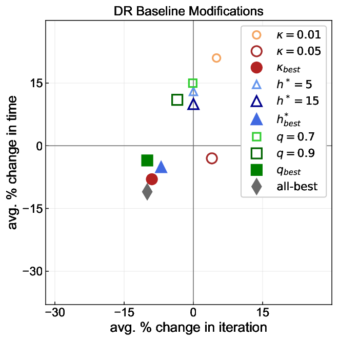
Comparing Figures 9(a) and 9(b), it appears that solution time is more sensitive to the parameters for trust regions and the early-stop heuristic than the parameters for the dimensionality reduction enhancement. This result is intuitive since trust regions and the early-stop heuristic yield much larger improvements when added to any algorithm (see Figure 4).
Based on the previous results, we derive a few general insights into parameter value choices for the trust regions and early stop heuristic:
- •
Trust region growth rate (). A significant gain in total solution time is observed when the trust region growth rate is high, i.e., . When the size of trust regions are increased too rapidly, the computational gains from solving smaller cut generation problems are generally reduced.
- •
Frequency of trust region removal (). The total solution time is higher when than when or . This observation suggests that removing trust regions too frequently may reduce the computational gains of faster cut generation, especially when trust regions are small.
- •
Early-stop value (). Cuts may be weaker when is decreased. For example, is the only parameter modification that leads to higher total iteration count. This is consistent with our theory, which suggests that the gain in cut strength when using trust regions comes from the computation of the extreme points of the corresponding subregion. When is low, an interior point of the subregion may be returned instead of an extreme point. Nonetheless, we observe through the progression of , (baseline) and that the improvement in cut generation speed generally outweighs the increase in iteration count from a lower value.
7.3 Takeaways from numerical results
The three main takeaways from our numerical results are: i) trust regions improve the strength of cuts and reduce cut generation time, particularly when trust regions are small, ii) the early-stop heuristic further reduces cut generation time, whereas the dimensionality reduction can help but comes with a potential cost of reducing the strength of cuts, iii) default parameter settings seem to work well, but additional tuning of algorithm parameters can lead to significant improvements in solution time.
8 Conclusion
In this paper, we develop a novel class of cutting plane algorithms for solving inverse MILO problems. Our approach of using trust regions to speed up computation is simple but effective, and is well-supported by our insights on the optimality conditions of inverse MILO problems. Through extensive computational experiments, we demonstrate that our cut generation techniques and enhancements are highly effective across a large range of inverse MILO problems.
References
- Afşar et al. (2021) Afşar, Sezin, Luce Brotcorne, Patrice Marcotte, Gilles Savard. 2021. Revenue optimization in energy networks involving self-scheduled demand and a smart grid. Computers & Operations Research 134 105366.
- Agarwal and Ergun (2010) Agarwal, Richa, Özlem Ergun. 2010. Network design and allocation mechanisms for carrier alliances in liner shipping. Operations research 58(6) 1726–1742.
- Ahuja and Orlin (2001) Ahuja, Ravindra K, James B Orlin. 2001. Inverse optimization. Operations Research 49(5) 771–783.
- Aswani et al. (2018) Aswani, Anil, Zuo-Jun Shen, Auyon Siddiq. 2018. Inverse optimization with noisy data. Operations Research 66(3) 870–892.
- Babier et al. (2021) Babier, Aaron, Timothy CY Chan, Taewoo Lee, Rafid Mahmood, Daria Terekhov. 2021. An ensemble learning framework for model fitting and evaluation in inverse linear optimization. Informs Journal on Optimization 3(2) 119–138.
- Babier et al. (2020) Babier, Aaron, Rafid Mahmood, Andrea L McNiven, Adam Diamant, Timothy CY Chan. 2020. Knowledge-based automated planning with three-dimensional generative adversarial networks. Medical Physics 47(2) 297–306.
- Bertsimas et al. (2012) Bertsimas, Dimitris, Vishal Gupta, Ioannis Ch Paschalidis. 2012. Inverse optimization: A new perspective on the black-litterman model. Operations research 60(6) 1389–1403.
- Bertsimas et al. (2015) Bertsimas, Dimitris, Vishal Gupta, Ioannis Ch Paschalidis. 2015. Data-driven estimation in equilibrium using inverse optimization. Mathematical Programming 153(2) 595–633.
- Birge et al. (2017) Birge, John R, Ali Hortaçsu, J Michael Pavlin. 2017. Inverse optimization for the recovery of market structure from market outcomes: An application to the miso electricity market. Operations Research 65(4) 837–855.
- Brotcorne et al. (2011) Brotcorne, Luce, Fabien Cirinei, Patrice Marcotte, Gilles Savard. 2011. An exact algorithm for the network pricing problem. Discrete Optimization 8(2) 246–258.
- Bulut and Ralphs (2015) Bulut, Aykut, Ted K Ralphs. 2015. On the complexity of inverse mixed integer linear optimization. Tech. rep., Tech. rep. COR@ L Laboratory Report 15T-001-R3, Lehigh University.
- Burton and Toint (1992) Burton, Didier, Ph L Toint. 1992. On an instance of the inverse shortest paths problem. Mathematical Programming 53(1-3) 45–61.
- Chan et al. (2014) Chan, Timothy CY, Tim Craig, Taewoo Lee, Michael B Sharpe. 2014. Generalized inverse multiobjective optimization with application to cancer therapy. Operations Research 62(3) 680–695.
- Chan and Kaw (2020) Chan, Timothy CY, Neal Kaw. 2020. Inverse optimization for the recovery of constraint parameters. European Journal of Operational Research 282(2) 415–427.
- Chan et al. (2019) Chan, Timothy CY, Taewoo Lee, Daria Terekhov. 2019. Inverse optimization: Closed-form solutions, geometry, and goodness of fit. Management Science 65(3) 1115–1135.
- Chen et al. (2021) Chen, Lu, Yuyi Chen, André Langevin. 2021. An inverse optimization approach for a capacitated vehicle routing problem. European Journal of Operational Research .
- Chow and Recker (2012) Chow, Joseph YJ, Will W Recker. 2012. Inverse optimization with endogenous arrival time constraints to calibrate the household activity pattern problem. Transportation Research Part B: Methodological 46(3) 463–479.
- Chow et al. (2014) Chow, Joseph YJ, Stephen G Ritchie, Kyungsoo Jeong. 2014. Nonlinear inverse optimization for parameter estimation of commodity-vehicle-decoupled freight assignment. Transportation Research Part E: Logistics and Transportation Review 67 71–91.
- Duan and Wang (2011) Duan, Zhaoyang, Lizhi Wang. 2011. Heuristic algorithms for the inverse mixed integer linear programming problem. Journal of Global Optimization 51(3) 463–471.
- Erkin et al. (2010) Erkin, Zeynep, Matthew D Bailey, Lisa M Maillart, Andrew J Schaefer, Mark S Roberts. 2010. Eliciting patients’ revealed preferences: an inverse markov decision process approach. Decision Analysis 7(4) 358–365.
- Esfahani et al. (2018) Esfahani, Peyman Mohajerin, Soroosh Shafieezadeh-Abadeh, Grani A Hanasusanto, Daniel Kuhn. 2018. Data-driven inverse optimization with imperfect information. Mathematical Programming 167(1) 191–234.
- Esfandeh et al. (2016) Esfandeh, Tolou, Changhyun Kwon, Rajan Batta. 2016. Regulating hazardous materials transportation by dual toll pricing. Transportation Research Part B: Methodological 83 20–35.
- Gleixner et al. (2019) Gleixner, Ambros, Gregor Hendel, Gerald Gamrath, Tobias Achterberg, Michael Bastubbe, Timo Berthold, Philipp M Christophel, Kati Jarck, Thorsten Koch, Jeff Linderoth, et al. 2019. Miplib 2017: Data-driven compilation of the 6th mixed-integer programming library. Optimization online preprint: http://www. optimization-online. org/DB_HTML/2019/07/7285. html. Submitted to Mathematical Programming Computation .
- Güler and Hamacher (2010) Güler, Çiğdem, Horst W Hamacher. 2010. Capacity inverse minimum cost flow problem. Journal of Combinatorial Optimization 19(1) 43–59.
- Heuberger (2004) Heuberger, Clemens. 2004. Inverse combinatorial optimization: A survey on problems, methods, and results. Journal of combinatorial optimization 8(3) 329–361.
- Houghtalen et al. (2011) Houghtalen, Lori, Özlem Ergun, Joel Sokol. 2011. Designing mechanisms for the management of carrier alliances. Transportation Science 45(4) 465–482.
- Iyengar and Kang (2005) Iyengar, Garud, Wanmo Kang. 2005. Inverse conic programming with applications. Operations Research Letters 33(3) 319–330.
- Keshavarz et al. (2011) Keshavarz, Arezou, Yang Wang, Stephen Boyd. 2011. Imputing a convex objective function. 2011 IEEE International Symposium on Intelligent Control. IEEE, 613–619.
- Kuiteing et al. (2017) Kuiteing, Aimé Kamgaing, Patrice Marcotte, Gilles Savard. 2017. Network pricing of congestion-free networks: The elastic and linear demand case. Transportation Science 51(3) 791–806.
- Kuiteing et al. (2018) Kuiteing, Aimé Kamgaing, Patrice Marcotte, Gilles Savard. 2018. Pricing and revenue maximization over a multicommodity transportation network: the nonlinear demand case. Computational Optimization and Applications 71(3) 641–671.
- Lamperski and Schaefer (2015) Lamperski, Jourdain B, Andrew J Schaefer. 2015. A polyhedral characterization of the inverse-feasible region of a mixed-integer program. Operations Research Letters 43(6) 575–578.
- Linderoth and Wright (2003) Linderoth, Jeff, Stephen Wright. 2003. Decomposition algorithms for stochastic programming on a computational grid. Computational Optimization and Applications 24(2-3) 207–250.
- Marcotte et al. (2009) Marcotte, Patrice, Anne Mercier, Gilles Savard, Vedat Verter. 2009. Toll policies for mitigating hazardous materials transport risk. Transportation science 43(2) 228–243.
- Naghavi et al. (2019) Naghavi, Mostafa, Ali Asghar Foroughi, Masoud Zarepisheh. 2019. Inverse optimization for multi-objective linear programming. Optimization Letters 13(2) 281–294.
- Rahmaniani et al. (2017) Rahmaniani, Ragheb, Teodor Gabriel Crainic, Michel Gendreau, Walter Rei. 2017. The benders decomposition algorithm: A literature review. European Journal of Operational Research 259(3) 801–817.
- Rathore and Jakhar (2021) Rathore, Himanshu, Suresh Kumar Jakhar. 2021. Differential carbon tax policy in aviation: One stone that kills two birds? Journal of Cleaner Production 296 126479.
- Ruiz et al. (2013) Ruiz, Carlos, Antonio J Conejo, Dimitris J Bertsimas. 2013. Revealing rival marginal offer prices via inverse optimization. IEEE Transactions on Power Systems 28(3) 3056–3064.
- Saez-Gallego et al. (2016) Saez-Gallego, Javier, Juan M Morales, Marco Zugno, Henrik Madsen. 2016. A data-driven bidding model for a cluster of price-responsive consumers of electricity. IEEE Transactions on Power Systems 31(6) 5001–5011.
- Schaefer (2009) Schaefer, Andrew J. 2009. Inverse integer programming. Optimization Letters 3(4) 483–489.
- Troutt et al. (2006) Troutt, Marvin D, Wan-Kai Pang, Shui-Hung Hou. 2006. Behavioral estimation of mathematical programming objective function coefficients. Management science 52(3) 422–434.
- Turner and Chan (2013) Turner, Sarina DO, Timothy CY Chan. 2013. Examining the leed rating system using inverse optimization. Journal of Solar Energy Engineering 135(4) 040901.
- Utz et al. (2014) Utz, Sebastian, Maximilian Wimmer, Markus Hirschberger, Ralph E Steuer. 2014. Tri-criterion inverse portfolio optimization with application to socially responsible mutual funds. European Journal of Operational Research 234(2) 491–498.
- Wang (2009) Wang, Lizhi. 2009. Cutting plane algorithms for the inverse mixed integer linear programming problem. Operations Research Letters 37(2) 114–116.
- Xu et al. (2018) Xu, Susan Jia, Mehdi Nourinejad, Xuebo Lai, Joseph YJ Chow. 2018. Network learning via multiagent inverse transportation problems. Transportation Science 52(6) 1347–1364.
- Yu et al. (2020) Yu, Shi, Haoran Wang, Chaosheng Dong. 2020. Learning risk preferences from investment portfolios using inverse optimization. arXiv preprint arXiv:2010.01687 .
- Zhang and Liu (1996) Zhang, Jianzhong, Zhenhong Liu. 1996. Calculating some inverse linear programming problems. Journal of Computational and Applied Mathematics 72(2) 261–273.
- Zhang and Xu (2010) Zhang, Jianzhong, Chengxian Xu. 2010. Inverse optimization for linearly constrained convex separable programming problems. European Journal of Operational Research 200(3) 671–679.
- Zhang et al. (2010) Zhang, Jianzhong, Liwei Zhang, Xiantao Xiao. 2010. A perturbation approach for an inverse quadratic programming problem. Mathematical Methods of Operations Research 72(3) 379–404.
- Zhang et al. (2018) Zhang, Jing, Sepideh Pourazarm, Christos G Cassandras, Ioannis Ch Paschalidis. 2018. The price of anarchy in transportation networks: Data-driven evaluation and reduction strategies. Proceedings of the IEEE 106(4) 538–553.
- Zhou et al. (2011) Zhou, Ying, Lizhi Wang, James D McCalley. 2011. Designing effective and efficient incentive policies for renewable energy in generation expansion planning. Applied Energy 88(6) 2201–2209.
- Zverovich et al. (2012) Zverovich, Victor, Csaba I Fábián, Eldon FD Ellison, Gautam Mitra. 2012. A computational study of a solver system for processing two-stage stochastic lps with enhanced benders decomposition. Mathematical Programming Computation 4(3) 211–238.
Appendix A Proofs
Several of the proofs in this section use the result that the inverse-feasible region of the sets , , and are the same, i.e., . This result was previously established in Wang 2009.
Proof A.1
Proof of Lemma 2.6
The main result that must be proved is that for any given , . Given that this statement is true, the result of comes trivially. The proof comes in two parts. we first prove that (i) for any given , . We then prove that (ii) for any given and , .
Proof: (i) Let . By definition, . Similarly, . Since , the statement must be true. (ii) For any and , let denote any vector such that , i.e., . Because is positive, . Thus, .
Proof A.2
Proof of Theorem 2.7
We prove by contradiction. () We assume , but is not a generator set. This implies that there exists some such that either (i) but or (ii) but . If (i) is true, then there exists a cost vector such that but for some . By definition, this cannot be in , i.e., , and thus . Furthermore, there cannot exist any such that . This implies that , which is a contradiction. The same argument can be applied to show that (ii) leads to a contradiction.
() We assume that is in fact a generator set, but . This implies that there exists a point such that either (i*) but or (ii*) but . If (i*) is true, then there exists a seperating hyperplane between and . The normal vector of this hyperplane that is pointing in the direction of defines a cost vector such that all points , which implies that . On the other hand, lies on the opposite side of the hyperplane, which implies that . Finally, because and thus must be constructed by a convex combination of the rays , there must exist at least one such that . This contradicts the initial assumption that . The same argument can be applied to show that (ii*) leads to a contradiction.
Proof A.3
Proof of Corollary 2.8 () Note that by the definition of , . If is a generator set, then by Theorem 2.7. Thus, . These statements together yield . () Suppose for some . This implies that for any , and . Therefore, . Since , the reverse must also be true, i.e., . Thus, . Applying Theorem 2.7, must be a generator set.
Proof A.4
Proof of Theorem 2.9
() We first prove the forward direction, i.e., that if is a generator set, then must be a subset of . We prove by contradiction. Suppose that there exists a point in such that . This implies that there exists a separating hyperplane between and . The point must lie in only of side of this hyperplane. Taking the normal vector of this hyperplane to be , we must have that either and , or that and . Given that , this contracts the initial assumption that .
() We now prove the reverse direction. In particular, we prove that if the convex hull of with contains the set for some , then must be a forward-feasible generator set, i.e., . We first observe that if , then
We will now prove that both sides of this equation can be simplied to obtain , at which point we can apply Corollary 2.8 to show that is a generator set. The major steps in this proof rely on the definition of the set , and we refer to Theorem 2.7 for its definition.
We first simplify the left side of the equation. Note that by the definition of , which is a set polyhedral cone pointed at , for any . This implies that , since . The set can be further simplified into by the definition of . We now simplify the right side of the equation. Given that by definition, the right side of the equation can be simplified to . Furthermore, .
These steps lead to the result that . Since , and we assumed , and by Corollary (2.8), must be a forward-feasible generator set.
Electronic Companion
Appendix B Approximations using Inverse Linear Optimization
Let denote a relaxed forward-feasible region where all integrality constraints present in are ignored. Similarly, let denote the solution to an arbitrary inverse linear optimization model where is considered instead of . Since , the inverse-feasible region must be a subset of , i.e., .
The main drawback of using inverse linear optimization over is that the set can be very different from the true inverse-feasible region . This means that can be very far from the (or in fact any) optimal solution . Furthermore, there can be a large number of different regions that define the same mixed integer set when the integrality constraints are considered. Specifically, for a fixed and generating , there can exist many different and that can replace and and generate the same . However, each of these ’s and ’s will generate different sets. This means that the estimates of are entirely dependent on the particular definition of and , making , and the quality of relative to , unstable.
For example, consider Figure 10, where the forward-feasible region in each of the subfigures are the same, i.e., . On the other hand, the linear constraints used to describe this region (, and the two hyperplanes indicated by orange lines) are different, resulting in different and very different inverse-feasible regions for the solution . In particular, the inverse-feasible regions of become increasingly smaller from Figures (1a) to (1d), which would result in solutions that become increasingly worse relative to for any choice of . This example, with in Figure (1d), also shows that there is no bound on the distance between and (or similarly, between and ). For these reasons, inverse linear optimization models may be poorly suited for solving inverse MILO models.
Appendix C Example of Algorithm Performance over a Single Instance
Below, we provide an example of the performance of the five algorithms over the instance assign1-5-8_t1. In Figure 11, the total solution time is plotted against the iteration count, and the slope of the line at any iteration reflects the cut generation speed at that particular iteration. The instance cannot be solved by CP, which has particularly high cut generation times, computing only 3 cuts by the one hour time limit. Adding the early-stop heuristic on CP (forming CP-ES) lowers cut generation times and results in a solution time of 2061 seconds with 250 iterations. On the other hand, adding trust regions on the CP (forming CPTR) lowers cut generation times more significant, and improves the strength of cuts, resulting in the instance being solved in 590 seconds while requiring only 81 iterations. We observe through Figure 11 that cut generation times are initially very low, and gradually increase with iteration count (as a result of larger trust regions). CPTR-ES further reduces cut generation time while requiring the same number of iterations. Finally, CPTR-ES-DR requires 9 more iterations than CPTR-ES, but the decrease in average cut generation time dominates the increase in iteration count.
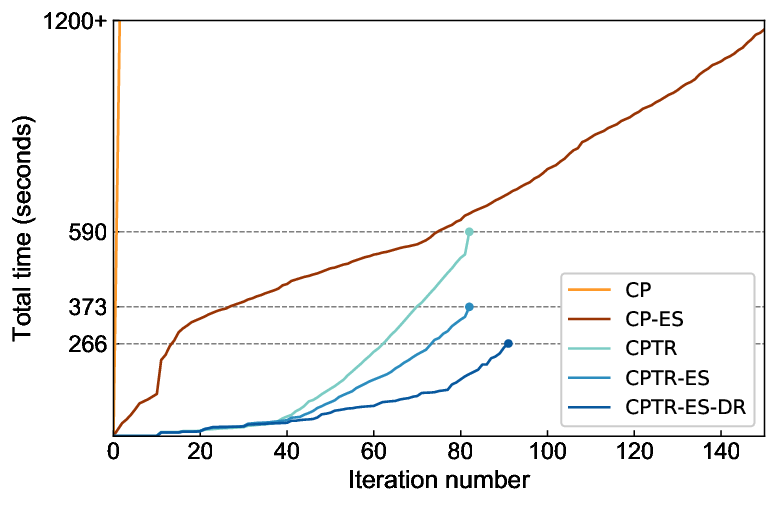
Appendix D Table of Solved Instances
| Problem Size | CP | CP-ES | CPTR | CPTR-ES | CPTR-ES-DR | |||||||
|---|---|---|---|---|---|---|---|---|---|---|---|---|
| Instance | vars. | cons. | num.it. | time(s) | num.it. | time(s) | num.it. | time(s) | num.it. | time(s) | num.it. | time(s) |
| 50v-10_t1 | 2013 | 233 | 0 | 3600 | 4964 | 3600 | 1567 | 1919 | 1265 | 206 | 2460 | 370 |
| 50v-10_t2 | 2013 | 233 | 0 | 3600 | 4567 | 3600 | 1002 | 992 | 990 | 121 | 1731 | 240 |
| 50v-10_t3 | 2013 | 233 | 0 | 3600 | 4732 | 3600 | 1456 | 237 | 1351 | 164 | 3046 | 402 |
| assign1-5-8_t1 | 156 | 161 | 2 | 3600 | 250 | 2061 | 81 | 590 | 81 | 372 | 90 | 266 |
| assign1-5-8_t2 | 156 | 161 | 4 | 3600 | 71 | 455 | 26 | 38 | 26 | 11 | 26 | 14 |
| assign1-5-8_t3 | 156 | 161 | 3 | 3600 | 139 | 682 | 50 | 46 | 50 | 47 | 69 | 290 |
| bppc4-08_t1 | 1456 | 111 | 0 | 3600 | 1 | 108 | 0 | 3600 | 1 | 108 | 1 | 108 |
| bppc4-08_t2 | 1456 | 111 | 0 | 3600 | 1 | 13 | 0 | 3600 | 1 | 11 | 1 | 11 |
| bppc4-08_t3 | 1456 | 111 | 0 | 3600 | 1 | 5 | 0 | 3600 | 1 | 5 | 1 | 6 |
| cod105_t1 | 1024 | 1024 | 5 | 3600 | 6 | 3600 | 10 | 3600 | 17 | 1894 | 27 | 2557 |
| cod105_t2 | 1024 | 1024 | 0 | 127 | 0 | 121 | 0 | 122 | 0 | 100 | 0 | 117 |
| cod105_t3 | 1024 | 1024 | 6 | 3600 | 9 | 3600 | 10 | 3600 | 18 | 1474 | 24 | 1916 |
| csched007_t2 | 1758 | 351 | 3 | 3600 | 256 | 3600 | 20 | 3600 | 147 | 3600 | 144 | 3475 |
| csched008_t1 | 1536 | 351 | 17 | 1533 | 23 | 260 | 4 | 666 | 5 | 64 | 6 | 91 |
| csched008_t2 | 1536 | 351 | 17 | 2137 | 115 | 2122 | 10 | 1489 | 40 | 2748 | 41 | 1164 |
| csched008_t3 | 1536 | 351 | 18 | 3600 | 193 | 2768 | 1 | 3600 | 26 | 130 | 53 | 2711 |
| cvs16r128-89_t2 | 3472 | 4633 | 0 | 3600 | 489 | 3600 | 6 | 3600 | 200 | 1260 | 270 | 963 |
| cvs16r128-89_t3 | 3472 | 4633 | 0 | 3600 | 483 | 3600 | 5 | 3600 | 170 | 1368 | 270 | 1680 |
| drayage-100-23_t1 | 11090 | 4630 | 660 | 3600 | 788 | 3600 | 174 | 245 | 174 | 274 | 195 | 242 |
| drayage-100-23_t2 | 11090 | 4630 | 935 | 3600 | 755 | 2370 | 124 | 218 | 124 | 247 | 150 | 235 |
| drayage-100-23_t3 | 11090 | 4630 | 492 | 3600 | 796 | 3600 | 160 | 3600 | 176 | 3600 | 178 | 3520 |
| drayage-25-23_t1 | 11090 | 4630 | 765 | 3600 | 861 | 3600 | 162 | 277 | 159 | 270 | 173 | 217 |
| drayage-25-23_t2 | 11090 | 4630 | 912 | 3303 | 875 | 2657 | 129 | 283 | 129 | 321 | 116 | 217 |
| drayage-25-23_t3 | 11090 | 4630 | 461 | 3600 | 821 | 3600 | 137 | 1069 | 139 | 659 | 172 | 684 |
| eil33-2_t1 | 4516 | 32 | 89 | 75 | 89 | 71 | 93 | 102 | 104 | 107 | 102 | 102 |
| eil33-2_t2 | 4516 | 32 | 86 | 101 | 86 | 88 | 87 | 127 | 97 | 142 | 116 | 161 |
| eil33-2_t3 | 4516 | 32 | 51 | 105 | 52 | 105 | 67 | 405 | 80 | 386 | 93 | 661 |
| enlight_hard_t1 | 200 | 100 | 0 | 0 | 0 | 0 | 0 | 0 | 0 | 0 | 0 | 0 |
| enlight_hard_t2 | 200 | 100 | 0 | 0 | 0 | 0 | 0 | 0 | 0 | 0 | 0 | 0 |
| enlight_hard_t3 | 200 | 100 | 0 | 0 | 0 | 0 | 0 | 0 | 0 | 0 | 0 | 0 |
| gen-ip002_t1 | 41 | 24 | 63 | 704 | 60 | 229 | 44 | 600 | 44 | 90 | 53 | 105 |
| gen-ip002_t2 | 41 | 24 | 28 | 615 | 28 | 51 | 34 | 559 | 34 | 44 | 44 | 52 |
| gen-ip002_t3 | 41 | 24 | 65 | 893 | 61 | 309 | 52 | 688 | 54 | 144 | 70 | 189 |
| germanrr_t1 | 10813 | 10779 | 0 | 3600 | 1 | 24 | 0 | 3600 | 1 | 21 | 1 | 23 |
| germanrr_t2 | 10813 | 10779 | 0 | 3600 | 1 | 16 | 0 | 3600 | 1 | 22 | 1 | 22 |
| germanrr_t3 | 10813 | 10779 | 0 | 3600 | 1 | 17 | 0 | 3600 | 1 | 22 | 1 | 22 |
| glass-sc_t1 | 214 | 6119 | 0 | 3600 | 292 | 3600 | 161 | 961 | 161 | 140 | 188 | 151 |
| glass-sc_t2 | 214 | 6119 | 0 | 3600 | 512 | 1826 | 125 | 1314 | 125 | 126 | 125 | 125 |
| glass-sc_t3 | 214 | 6119 | 0 | 3600 | 640 | 2074 | 131 | 1704 | 136 | 146 | 136 | 145 |
| gmu-35-40_t1 | 1205 | 424 | 593 | 934 | 411 | 176 | 93 | 1323 | 96 | 137 | 98 | 143 |
| gmu-35-50_t2 | 1919 | 435 | 442 | 3600 | 621 | 292 | 86 | 1270 | 86 | 45 | 87 | 43 |
| gmu-35-50_t3 | 1919 | 435 | 3 | 3600 | 699 | 284 | 10 | 3600 | 87 | 74 | 102 | 89 |
| leo1_t1 | 6731 | 593 | 1 | 359 | 1 | 5 | 1 | 351 | 1 | 5 | 1 | 6 |
| leo1_t2 | 6731 | 593 | 1 | 395 | 1 | 5 | 1 | 351 | 1 | 5 | 1 | 7 |
| leo1_t3 | 6731 | 593 | 0 | 198 | 0 | 203 | 0 | 182 | 0 | 209 | 0 | 207 |
| leo2_t1 | 11100 | 593 | 1 | 919 | 1 | 6 | 1 | 887 | 1 | 6 | 1 | 7 |
| leo2_t2 | 11100 | 593 | 1 | 1034 | 1 | 5 | 1 | 885 | 1 | 6 | 1 | 7 |
| leo2_t3 | 11100 | 593 | 0 | 496 | 1 | 5 | 0 | 432 | 1 | 11 | 1 | 11 |
| markshare_4_0_t1 | 34 | 4 | 4 | 0 | 4 | 0 | 4 | 0 | 4 | 0 | 4 | 0 |
| markshare_4_0_t2 | 34 | 4 | 4 | 0 | 4 | 0 | 4 | 0 | 4 | 0 | 4 | 0 |
| markshare_4_0_t3 | 34 | 4 | 8 | 2 | 8 | 2 | 9 | 1 | 9 | 2 | 9 | 2 |
| markshare2_t1 | 74 | 7 | 0 | 3600 | 8 | 7 | 0 | 3600 | 8 | 5 | 8 | 5 |
| markshare2_t2 | 74 | 7 | 0 | 3600 | 7 | 7 | 0 | 3600 | 7 | 5 | 7 | 5 |
| markshare2_t3 | 74 | 7 | 0 | 3600 | 8 | 8 | 0 | 3600 | 8 | 5 | 8 | 5 |
| mas74_t1 | 151 | 13 | 21 | 445 | 1 | 5 | 1 | 0 | 1 | 0 | 1 | 0 |
| mas74_t2 | 151 | 13 | 21 | 467 | 1 | 5 | 1 | 0 | 1 | 0 | 1 | 0 |
| mas74_t3 | 151 | 13 | 21 | 458 | 1 | 5 | 1 | 0 | 1 | 0 | 1 | 0 |
| mas76_t1 | 151 | 12 | 16 | 20 | 1 | 21 | 1 | 0 | 1 | 0 | 1 | 0 |
| mas76_t2 | 151 | 12 | 16 | 21 | 1 | 21 | 1 | 0 | 1 | 0 | 1 | 0 |
| mas76_t3 | 151 | 12 | 16 | 21 | 1 | 22 | 1 | 0 | 1 | 0 | 1 | 0 |
| mcsched_t1 | 1747 | 2107 | 1 | 90 | 1 | 7 | 1 | 88 | 1 | 7 | 1 | 7 |
| mcsched_t2 | 1747 | 2107 | 1 | 93 | 1 | 7 | 1 | 88 | 1 | 7 | 1 | 7 |
| mcsched_t3 | 1747 | 2107 | 1 | 135 | 1 | 11 | 1 | 131 | 1 | 11 | 1 | 11 |
| mik-250-20-75-4_t1 | 270 | 195 | 2626 | 580 | 2626 | 624 | 121 | 4 | 131 | 7 | 124 | 7 |
| mik-250-20-75-4_t2 | 270 | 195 | 2336 | 3600 | 2312 | 3600 | 154 | 145 | 161 | 161 | 170 | 171 |
| mik-250-20-75-4_t3 | 270 | 195 | 2480 | 451 | 2480 | 484 | 191 | 13 | 185 | 10 | 191 | 12 |
| mzzv11_t1 | 10240 | 9499 | 616 | 3600 | 640 | 3600 | 109 | 653 | 118 | 604 | 137 | 568 |
| mzzv11_t2 | 10240 | 9499 | 765 | 3600 | 732 | 3181 | 104 | 423 | 99 | 404 | 112 | 453 |
| mzzv11_t3 | 10240 | 9499 | 723 | 3600 | 689 | 3318 | 132 | 698 | 156 | 815 | 152 | 527 |
| mzzv42z_t1 | 11717 | 10460 | 764 | 2624 | 777 | 3027 | 86 | 258 | 93 | 292 | 112 | 259 |
| mzzv42z_t2 | 11717 | 10460 | 740 | 2208 | 788 | 2326 | 100 | 186 | 103 | 257 | 111 | 186 |
| mzzv42z_t3 | 11717 | 10460 | 953 | 3600 | 945 | 3600 | 80 | 230 | 90 | 285 | 102 | 314 |
| n5-3_t1 | 2550 | 1062 | 8994 | 2167 | 7731 | 1889 | 1432 | 245 | 737 | 121 | 816 | 213 |
| n5-3_t2 | 2550 | 1062 | 5645 | 1301 | 4945 | 982 | 396 | 108 | 842 | 138 | 595 | 173 |
| n5-3_t3 | 2550 | 1062 | 5866 | 1159 | 5544 | 988 | 397 | 99 | 2355 | 461 | 495 | 163 |
| neos-2657525-crna_t2 | 524 | 342 | 0 | 3600 | 19 | 116 | 0 | 3600 | 18 | 55 | 18 | 55 |
| neos-3083819-nubu_t1 | 8644 | 4725 | 403 | 1265 | 319 | 1009 | 180 | 537 | 162 | 533 | 156 | 304 |
| neos-3083819-nubu_t2 | 8644 | 4725 | 116 | 1768 | 273 | 1977 | 116 | 1094 | 218 | 1967 | 145 | 777 |
| neos-3083819-nubu_t3 | 8644 | 4725 | 364 | 2854 | 250 | 1837 | 165 | 244 | 188 | 343 | 193 | 243 |
| neos-3381206-awhea_t2 | 2375 | 479 | 104 | 3600 | 1490 | 3600 | 119 | 3600 | 379 | 3597 | 330 | 3177 |
| neos-3627168-kasai_t1 | 1462 | 1655 | 0 | 3600 | 3 | 36 | 0 | 3600 | 3 | 36 | 4 | 11 |
| neos-3627168-kasai_t2 | 1462 | 1655 | 0 | 3600 | 3 | 33 | 0 | 3600 | 3 | 34 | 4 | 11 |
| neos-3627168-kasai_t3 | 1462 | 1655 | 0 | 3600 | 3 | 69 | 0 | 3600 | 3 | 64 | 3 | 34 |
| neos-4338804-snowy_t1 | 1344 | 1701 | 0 | 3600 | 614 | 105 | 36 | 2 | 36 | 2 | 39 | 6 |
| neos-4338804-snowy_t2 | 1344 | 1701 | 0 | 3600 | 1079 | 652 | 37 | 8 | 37 | 8 | 62 | 9 |
| neos-4338804-snowy_t3 | 1344 | 1701 | 0 | 3600 | 1453 | 1391 | 95 | 50 | 95 | 51 | 143 | 60 |
| neos-4954672-berkel_t1 | 1533 | 1848 | 0 | 3600 | 1909 | 3600 | 10 | 3600 | 455 | 258 | 476 | 322 |
| neos-4954672-berkel_t2 | 1533 | 1848 | 0 | 3600 | 3511 | 3600 | 10 | 3600 | 424 | 205 | 462 | 215 |
| neos-4954672-berkel_t3 | 1533 | 1848 | 0 | 3600 | 1423 | 3600 | 10 | 3600 | 549 | 1601 | 567 | 1547 |
| neos-860300_t1 | 1385 | 850 | 20 | 139 | 16 | 58 | 20 | 101 | 24 | 86 | 33 | 192 |
| neos-860300_t2 | 1385 | 850 | 19 | 122 | 20 | 66 | 31 | 165 | 35 | 144 | 40 | 162 |
| neos-860300_t3 | 1385 | 850 | 17 | 185 | 28 | 180 | 22 | 172 | 25 | 146 | 24 | 193 |
| neos17_t2 | 535 | 486 | 2457 | 3600 | 675 | 1770 | 65 | 252 | 139 | 1612 | 144 | 238 |
| neos17_t3 | 535 | 486 | 441 | 3600 | 536 | 3221 | 150 | 974 | 155 | 1958 | 152 | 556 |
| neos5_t1 | 63 | 63 | 6 | 3600 | 69 | 688 | 38 | 0 | 38 | 0 | 38 | 0 |
| neos5_t2 | 63 | 63 | 71 | 1318 | 67 | 470 | 36 | 0 | 36 | 0 | 36 | 0 |
| neos5_t3 | 63 | 63 | 84 | 3343 | 81 | 2760 | 38 | 0 | 38 | 0 | 38 | 0 |
| qap10_t1 | 4150 | 1820 | 19 | 514 | 35 | 568 | 24 | 641 | 34 | 579 | 34 | 585 |
| qap10_t2 | 4150 | 1820 | 23 | 461 | 32 | 428 | 30 | 571 | 39 | 543 | 39 | 542 |
| qap10_t3 | 4150 | 1820 | 27 | 451 | 27 | 264 | 37 | 854 | 51 | 1022 | 51 | 1063 |
| ran14x18-disj-8_t1 | 504 | 447 | 0 | 3600 | 994 | 726 | 625 | 180 | 662 | 96 | 731 | 96 |
| ran14x18-disj-8_t2 | 504 | 447 | 0 | 3600 | 1777 | 1289 | 569 | 88 | 569 | 95 | 685 | 103 |
| ran14x18-disj-8_t3 | 504 | 447 | 0 | 3600 | 1250 | 788 | 563 | 110 | 522 | 60 | 667 | 71 |
| rocI-4-11_t1 | 6839 | 10883 | 1 | 268 | 1 | 296 | 1 | 321 | 1 | 369 | 1 | 368 |
| rocI-4-11_t2 | 6839 | 10883 | 2 | 368 | 2 | 318 | 2 | 681 | 2 | 668 | 2 | 645 |
| rocI-4-11_t3 | 6839 | 10883 | 3 | 226 | 5 | 83 | 3 | 146 | 4 | 56 | 4 | 63 |
| rococoB10-011000_t1 | 4456 | 1667 | 0 | 3600 | 1 | 9 | 0 | 3600 | 1 | 9 | 1 | 9 |
| rococoB10-011000_t2 | 4456 | 1667 | 0 | 3600 | 1 | 9 | 0 | 3600 | 1 | 9 | 1 | 9 |
| rococoB10-011000_t3 | 4456 | 1667 | 0 | 3600 | 1 | 11 | 0 | 3600 | 1 | 10 | 1 | 10 |
| rococoC10-001000_t1 | 3117 | 1293 | 1 | 261 | 1 | 10 | 1 | 335 | 1 | 9 | 1 | 10 |
| rococoC10-001000_t2 | 3117 | 1293 | 1 | 269 | 1 | 10 | 1 | 335 | 1 | 9 | 1 | 10 |
| rococoC10-001000_t3 | 3117 | 1293 | 1 | 270 | 1 | 10 | 1 | 335 | 1 | 9 | 1 | 10 |
| roi2alpha3n4_t1 | 6816 | 1251 | 20 | 3600 | 154 | 3600 | 149 | 3600 | 146 | 1599 | 142 | 1455 |
| roi2alpha3n4_t2 | 6816 | 1251 | 21 | 3600 | 197 | 3600 | 130 | 3600 | 125 | 524 | 144 | 3294 |
| roi2alpha3n4_t3 | 6816 | 1251 | 20 | 3600 | 155 | 3600 | 117 | 3600 | 146 | 2830 | 148 | 3537 |
| roll3000_t1 | 1166 | 2295 | 1 | 9 | 1 | 10 | 1 | 13 | 2 | 23 | 2 | 20 |
| roll3000_t2 | 1166 | 2295 | 10 | 168 | 5 | 81 | 5 | 83 | 5 | 72 | 5 | 80 |
| roll3000_t3 | 1166 | 2295 | 1 | 7 | 1 | 7 | 1 | 0 | 1 | 5 | 1 | 5 |
| seymour_t1 | 1372 | 4944 | 0 | 3600 | 443 | 3600 | 10 | 3600 | 1136 | 449 | 1426 | 431 |
| seymour_t2 | 1372 | 4944 | 0 | 3600 | 474 | 3600 | 10 | 3600 | 959 | 272 | 1036 | 253 |
| seymour_t3 | 1372 | 4944 | 0 | 3600 | 450 | 3600 | 30 | 3600 | 1194 | 614 | 1532 | 643 |
| seymour1_t1 | 1372 | 4944 | 47 | 3600 | 331 | 3600 | 1679 | 800 | 1543 | 521 | 1663 | 454 |
| seymour1_t2 | 1372 | 4944 | 48 | 3600 | 396 | 3600 | 956 | 495 | 970 | 263 | 1000 | 238 |
| seymour1_t3 | 1372 | 4944 | 49 | 3600 | 410 | 3600 | 1669 | 920 | 1669 | 496 | 1875 | 498 |
| sp150x300d_t1 | 600 | 450 | 4424 | 3600 | 1414 | 133 | 248 | 35 | 248 | 36 | 205 | 24 |
| sp150x300d_t2 | 600 | 450 | 2035 | 181 | 2035 | 181 | 222 | 26 | 222 | 29 | 228 | 19 |
| sp150x300d_t3 | 600 | 450 | 1653 | 193 | 1606 | 154 | 199 | 18 | 199 | 19 | 212 | 27 |
| splice1k1_t1 | 3253 | 6505 | 0 | 3600 | 1 | 48 | 0 | 3600 | 1 | 40 | 1 | 50 |
| splice1k1_t2 | 3253 | 6505 | 0 | 3600 | 1 | 47 | 0 | 3600 | 1 | 49 | 1 | 41 |
| splice1k1_t3 | 3253 | 6505 | 0 | 3600 | 1 | 48 | 0 | 3600 | 1 | 40 | 1 | 50 |
| supportcase26_t1 | 436 | 870 | 38 | 729 | 36 | 37 | 16 | 3 | 16 | 3 | 16 | 3 |
| supportcase26_t2 | 436 | 870 | 13 | 3600 | 70 | 2018 | 29 | 1537 | 30 | 686 | 34 | 950 |
| supportcase26_t3 | 436 | 870 | 9 | 487 | 14 | 8 | 3 | 0 | 3 | 0 | 3 | 0 |
| wachplan_t1 | 3361 | 1553 | 0 | 1787 | 0 | 1845 | 0 | 1123 | 0 | 1087 | 0 | 1087 |
| wachplan_t2 | 3361 | 1553 | 0 | 1804 | 0 | 1823 | 0 | 1122 | 0 | 1131 | 0 | 1135 |
| wachplan_t3 | 3361 | 1553 | 0 | 1799 | 0 | 1823 | 0 | 1123 | 0 | 1089 | 0 | 1133 |