Regularization by Denoising via Fixed-Point Projection (RED-PRO)
Abstract
Inverse problems in image processing are typically cast as optimization tasks, consisting of data fidelity and stabilizing regularization terms. A recent regularization strategy of great interest utilizes the power of denoising engines. Two such methods are the Plug-and-Play Prior (PnP) and Regularization by Denoising (RED). While both have shown state-of-the-art results in various recovery tasks, their theoretical justification is incomplete. In this paper, we aim to bridge between RED and PnP, enriching the understanding of both frameworks. Towards that end, we reformulate RED as a convex optimization problem utilizing a projection (RED-PRO) onto the fixed-point set of demicontractive denoisers. We offer a simple iterative solution to this problem, by which we show that PnP proximal gradient method is a special case of RED-PRO, while providing guarantees for the convergence of both frameworks to globally optimal solutions. In addition, we present relaxations of RED-PRO that allow for handling denoisers with limited fixed-point sets. Finally, we demonstrate RED-PRO for the tasks of image deblurring and super-resolution, showing improved results with respect to the original RED framework.
keywords
Inverse problems, Image denoising, Plug and Play Prior (PnP), Regularization by Denoising (RED), Demicontractive mappings, Fixed-point set.AMS
62H35, 68U10, 94A08, 65F10, 65F22, 47A52.1 Introduction
Inverse problems arise in numerous fields, ranging from astrophysics and optics to signal processing, computer vision and medical imaging [30, 29, 28, 81, 31, 62, 26]. Specifically to computational imaging, inverse problems relate to the task of inferring an unknown image from its corrupted measurements. Assuming a known degradation model (i.e., the forward operator), one may offer a formulation of the recovery process as an optimization problem comprising a data fidelity term. Unfortunately, this by itself is typically insufficient, as it leads to an ill-posed problem with a non-stable solution. To overcome this difficulty, regularization methods have been widely developed and used. A proper regularization enables a robust recovery by leveraging prior information on the unknown image, incorporated into the optimization formulation. Therefore, formulating and solving inverse problems often reduces to determining the appropriate regularization, depending on the specific application and the underlying signals in mind.
Many regularization schemes for natural images are available, and it is beyond the scope of this paper to review this rich literature. The focus of this paper is on the fascinating recent idea that image denoisers could be used as the mechanism behind the regularization term [77, 92]. Image denoising is the simplest known inverse problem, concerned with obtaining a clean image from its noisy measurements contaminated with additive noise, typically assumed to be zero-mean Gaussian distributed. Over the past decade, image denoising has been studied extensively, leading to a vast line of works (,e.g., [87, 42, 32, 85, 63, 35, 38, 24, 17, 58, 57, 54, 86, 49, 36, 73, 104, 25, 102, 50, 55, 80]). This has resulted in the availability of extremely efficient and effective algorithms, achieving nearly optimal performance [23, 59, 60].
The first to propose leveraging the power of denoising for regularization were Venkatakrishnan et al., presenting their Plug-and-Play Prior (PnP) framework [92, 22, 82]. PnP relies on the alternating direction method of multipliers (ADMM) for solving general inverse problems, and their method amounts to an iterative technique that decomposes the optimization problem into a sequence of simple denoising operations, known as proximal algorithms [71, 10]. The PnP approach replaces the proximal operators with state-of-the-art denoisers, thus, embodying implicit priors for regularizing inverse problems. This framework has gained great interest due to its success in various applications [82, 94, 75, 53, 105, 1, 95], and it has been extended to other proximal algorithms such as proximal gradient method (PGM) [11, 71], approximate message passing (AMP) [69, 12, 43, 39, 9] and half quadratic splitting [103]. Schemes similar to PnP has been proposed in [33] and [40], where the former is based on the augmented Lagrangian method and the latter relies on the notion of Nash equilibrium.
Despite its empirical success, when the denoising engines are more general than proximal maps, PnP loses its interpretability as a minimizer of explicit objective functions. While general inversion extends beyond optimization-based solutions, the existence of an underlying energy function being minimized benefits from extensive theoretical results and adds to the quality of the resulting algorithms, since it allows to properly tune the parameters, to incorporate line search and other acceleration methods, to analyze convergence better and understand the characteristics of the solutions. Nonetheless, several studies have proven the fixed-point convergence of variants of PnP under various assumptions. Chan et al. [22] proved the convergence of PnP-ADMM with increasing penalty parameter under the assumption of bounded denoisers. A similar condition was used in [90] for the analysis of a variant of PnP. In [18], PnP has been explained via the framework of consensus equilibrium, proving the convergence of PnP for nonexpansive denoisers. The latter has been the core assumption in multiple works [82, 84, 88, 21, 89], which proved the convergence of several PnP techniques by reformulating them as fixed-point iterations of (averaged) nonexpansive mappings. In [79], the authors relaxed this assumption to a certain Lipschitz condition. Yet, none of the above proved the convergence of PnP to global minima of an explicit objective function when the denoisers extend beyond proximal operators. Recently, the authors of [97] have proven, based on [47, 46, 48], that PnP with minimum mean squared error (MMSE) denoisers provably converges to an explicit, possibly nonconvex, cost function. However, this work assumes that the denoiser is infinitely differentiable with a symmetric Jacobian [48].
As a partial remedy and an enrichment to the above, Romano et al. introduced an alternative approach called Regularization by Denoising (RED) [77]. Here, a denoiser engine is utilized to form an explicit regularizer, consisting of the inner product between the unknown image and its denoising residual. Interestingly, under certain conditions, the RED prior defines a convex function whose gradient is simply given by the denoising residual itself. Thus, this gradient can be used by first-order optimization methods such as steepest decent (SD), fixed-point (FP) iteration and ADMM, leading to a convergence to the globally optimal solution of the regularized inverse problem.
The RED framework aims at formulating a clear and well-defined objective function, and has demonstrated state-of-the-art results in image deblurring and super-resolution, drawing a broad attention [74, 83, 66, 52, 94, 72, 103, 104]. However, RED formulation requires the denoiser to be differentiable, obey a local-homogeneity property, and have a symmetric Jacobian; conditions which are not met by various powerful denoisers [74], such as non-local means (NLM) [16], block-matching and 3D filtering (BM3D) [32], trainable nonlinear reaction-diffusion (TNRD) [25], and denoising convolutional neural network (DnCNN) [102]. In such cases, RED algorithms cease to act as optimization solvers and are deprived from their convergence guarantees to global optimum. To overcome this, Reehorst and Schniter introduced a framework called score-matching by denoising (SMD) [74], which offers a new interpretation of RED algorithms and proves their converge to a fixed-point assuming nonexpansive denoisers. In [83], a block coordinate RED algorithm was presented, including an analysis of its fixed-point convergence under the condition that the denoiser is block-nonexpansive. These works, however, did not show convergence to global minima of an explicit energy function.
As becomes clear from the above, the convergence analysis and the study of the solutions of both PnP and RED frameworks are incomplete. In this paper, our main goal is to enrich the theoretical understanding of PnP and RED by offering a new interpretation for their regularization strategy. Another objective we pose is the formation of a theoretical bridge between RED and PnP. While both RED and PnP have been interpreted as equilibrium consensus [74, 1, 18], here, we first establish a relationship between the two frameworks from an optimization point of view. The main contributions of this paper are two-fold:
- •
We re-introduce RED via the Fixed-Point Projection (RED-PRO) strategy. More specifically, given a convex objective function and a chosen denoiser , we formulate the following inverse problem
(1) Surprisingly, while the proposed regularization term is highly nonlinear, the problem above is convex for demicontractive denoisers with non-empty fixed-point set. We present a simple provably-convergent iterative technique to solve the resulting problem, and show that PnP proximal gradient is a special case of it. Moreover, we relate the family of demicontractive operators to previous common assumptions such as nonexpansiveness and boundedness, showing that the condition of demicontractivity covers a broader range of functions. The presented RED-PRO framework joins the PnP and RED approaches, offering an increased flexibility in choosing the denoiser, while preserving global convergence guarantees.
- •
Furthermore, we propose relaxations of RED-PRO that enable the use of denoisers with a narrow fixed-point set at the expense of higher computational load. Results of this strategy on the image deblurring and super-resolution problems show improved performance in comparison to the RED framework.
In addition to the above, we complement the work in [74] by considering the original RED framework where the denoiser is non-differentiable. We formulate the regularization as the Rockafellar function [76], and prove that under certain monotonicity condition on the denoiser, the proposed objective is a convex function, minimized by the RED algorithms. Thus, we provide guarantees for convergence of the RED framework to the globally optimal solution, while relieving the earlier conditions on differentiability, symmetry and homogeneity of the denoiser. As this part deviates from the main theme of this paper, it is brought in appendix B.
The remainder of the paper is organized as follows. Section 2 details preliminaries of inverse problems and briefly overviews the PnP and RED approaches. In Section 3, we review important results of fixed-point theory and discuss demicontractive denoisers extensively. Section 4 serves as the central part of this work. We introduce the RED-PRO framework, which exploits the fixed-point set of denoisers to solve general structured inverse problems. We discuss the relation between the proposed scheme and the PnP approach, including convergence guarantees. Relaxed versions of RED-PRO are presented, so as to allow handling denoisers with a narrow fixed-point set. Section 5 brings experimental results on image deblurring and super-resolution, demonstrating an improvement of the relaxed RED-PRO framework over the original RED algorithms. Finally, we conclude the paper in Section 6.
2 Preliminaries
In this section we provide the groundwork for this study. First, we describe the framework of inverse problems in image processing, formulated as optimization problems where the challenge is in determining the appropriate regularizer. Then, we discuss PnP and RED, which utilize denoising engines for regularization.
2.1 Inverse Problems
We consider the task of recovering an unknown image from its corrupted measurements . The Bayesian maximum a posteriori (MAP) estimator seeks for a solution that maximizes the posterior conditional probability
| (2) |
The latter can be simplified using Bayes’s rule as follows:
| (3) | ||||
where we omit since it is not a function of , and we exploit the monotonic decreasing property of to recast the estimation as a minimization problem. The log-likelihood term, denoted as , describes the probabilistic relationship between the measurements and the desired image , assumed to be known. Typically, the likelihood alone is not sufficient and leads to an ill-posed problem for which the solution is not unique or stable. The probability distribution leads to a prior, denoted by , incorporating the statistical nature of the unknown. This regularization term stabilizes and better-conditions the optimization problem. Thus, we can rewrite (3) as
| (4) |
where represents the level of confidence in the prior. We assume hereafter that the log-likelihood is a convex, differentiable, lower semicontinuous (l.s.c) and proper function. A classic model for the measurements, considered throughout this paper, is given by
| (5) |
where is a linear degradation operator and is a white Gaussian noise (WGN) of variance . This leads to
| (6) |
Note that the noise distribution might be different, e.g., Laplacian, Gamma-distributed, Poisson, and other noise models. In these cases, the expression for the log-likelihood above changes accordingly, differing from the -norm.
A challenge that remains is determining the prior to incorporate into the problem formulation. This task of choosing the appropriate has been the center of numerous studies, and various terms have been proposed, ranging from Tikhonov smoothness [44] and the classic Laplacian [56], through wavelet sparsity [64] and total variation [78], to patch-based GMM [107, 101], sparse-representation modeling [15, 41] and recent deep-learning techniques [91]. A possible answer to this challenge may lay in the solution of a special inverse problem, which is image denoising:
| (7) |
To a large extent, the removal of an additive white Gaussian noise from an image is considered in computational imaging as a solved problem [77]. In the last decade, many extremely effective image denoising algorithms have been proposed, yielding impressive results. In general, the image denoising engine is a function that maps an image to a different image of the same size, , where ideally – the original noiseless image. Denoising solutions may be based on the MAP estimation (7), minimum mean-square-error, collaborative filtering, supervised learning, and more. The success in noise removal has led researchers to exploit the power of denoising engines for solving other problems. In the following, we describe two approaches, PnP [92] and RED [77], which utilize denoisers as implicit and explicit regularization terms respectively. When the chosen denoisers are proximal operators PnP reduces to common solvers. Thus, the PnP framework extends well-known optimization schemes, while RED presents an alternative to them. When powerful denoiser are used, both these important approaches have shown state-of-the-art performance in tasks such as unsupervised image deblurring and image super-resolution.
2.2 Plug and Play Prior (PnP)
Here we briefly review the PnP approach [92] by Venkatakrishnan et al., who suggested the use of denoisers as an implicit regularization. We start with problem (4) where we assume that is convex. The MAP solution can be obtained by two common optimization solvers, PGM and ADMM, summarized in algorithm 1 and algorithm 2 respectively. Note that when , algorithm 1 reduces to the standard PGM method, while the following update rule
leads to the accelerated PGM [11].
- •
- •
- •
- •
- •
- •
As can be seen, both techniques make use of proximal operators, defined as
| (8) |
for a closed, proper and convex function . Notice that (8) resembles (7), implying that proximal operators are a specific family of denoisers. Thus, the PnP framework offers to extend algorithm 1 and algorithm 2 by replacing the proximal operators with a general denoiser,11 1 We use hereafter the function to denote a general denoiser, and we omit its dependency on the noise-level (or the denoising strength to employ). However, we should note that this parameter should be chosen carefully, as it can be critical for the performance of any of the algorithms described. , not necessarily variational in nature, i.e., a denoiser which is not originated from any explicit regularizer. This leads to PnP-PGM and PnP-ADMM, where the latter has been introduced in the original PnP formulation [92]. Note that the PnP-PGM requires the gradient of , while in general any method that evaluates the proximal operator of (rather than its gradient), e.g. PnP-ADMM, is more computationally expensive [84].
Empirically, incorporating powerful denoisers (such as BM3D, TNRD and DnCNN) into the PnP framework has led to state-of-the-art results in various inverse problems. However, for general denoisers other than proximal operators, the PnP methods cannot be interpreted as optimization solvers, making it difficult to theoretically investigate the stability and uniqueness of their solutions. Several studies [84, 22, 18, 88, 21, 89, 37, 90, 79] proved the convergence of PnP methods to a fixed-point under different conditions, while the work reported in [82] states clear conditions for a global convergence of PnP. Yet, none of these provide an explicit expression of an objective function which is minimized. In Section 4 we remedy this by introducing an optimization technique, which PnP-PGD is a special case of. Thus, we offer a novel theoretical explanation for PnP approach.
2.3 Regularization by Denoising (RED)
As discussed above, the PnP framework has been the first to exploit denoisers for an implicit regularization, while lacking an underlying objective function. As an alternative, Romano et al. [77] introduced a different, yet related, strategy that harnesses image denoisers, called REgularization by Denoising. The RED framework defines the following regularization term:
| (9) |
This prior is an image-adaptive Laplacian whose definition is based on the denoiser of choice, . Thus, the overall optimization problem to solve is
| (10) |
The denoiser is assumed to obey the following assumptions, which we refer to hereafter as the RED conditions
- (C1)
Local Homogeneity: , for sufficiently small .
- (C2)
Differentiability: The denoiser is differentiable where denotes its Jacobian.
- (C3)
Jacobian Symmetry [74]: .
- (C4)
Strong Passivity: The spectral radius the Jacobian satisfies .
Interestingly, under these conditions, the regularization term (9) is differentiable, convex, and its gradient is given by the denoising residual . Furthermore, denoting by the objective function of (10), is convex whenever the log- likelihood is convex, and it gradient is given simply as
| (11) |
Based on this expression, Romano et al. have proposed several iterative algorithms – steepest descent, fixed-point iteration and ADMM, which are guaranteed to converge to the global optimum of (10).
In a later work [74], the authors have argued that many popular denoisers lack symmetric Jacobian (C3),22 2 Indeed, [74] was the first work to draw attention to the need for symmetry of the Jacobian. making the gradient expression (11) invalid. Moreover, they have proven that when the denoiser fails to satisfy condition (C3), there is no regularizer whose gradient is the denoising residual . Yet, in practice, the RED algorithms converge and have demonstrated state-of-the-art results in super-resolution and image deblurring even when used with denoisers that are not differentiable, let alone exhibit symmetric Jacobian. Therefore, the theoretical justification of the RED approach remains an open question, which we aim to address in appendix B.
3 Demicontractivity
In this section, we introduce our assumption of demicontractive denoisers which is the fundamental building block of our framework formulation. We first outline basic definitions and facts of nonlinear analysis, followed by an extensive discussion on demicontractivity and its relation to other assumptions, motivating our work.
3.1 Fixed-Point Theory
Here we review key concepts of fixed-point theory [76, 7] on which we base our contributions. We start with considering a nonlinear mapping , and we say a point is a fixed-point of iff . We define the the set of all fixed-points of as
| (12) |
Throughout the paper we assume that is nonempty.33 3 A reasonable assumption is that as any denoiser of the form satisfies this. Moreover, all the denoisers we experiment with in this work meet this condition. Our study focuses on the set and its favorable properties for the family of demicontractive mappings defined next.
Definition 1 (Demicontractive).
The mapping is demicontractive with a constant (or -demicontractive) if for any and it holds that
| (13) |
or equivalently
| (14) |
Definition 2.
The mapping is quasi-nonexpansive if
| (15) |
We say is -strongly quasi-nonexpansive with if
| (16) |
Proposition 3.
Let be a -strongly quasi-nonexpansive mapping with . Then,
| (17) |
where represents the projection onto the fixed-point set of .
Definition 4.
The mapping is called nonexpansive if
| (18) |
Definition 5.
The mapping is Lipschitz continuous with a constant if
| (19) |
When , is called a contraction.
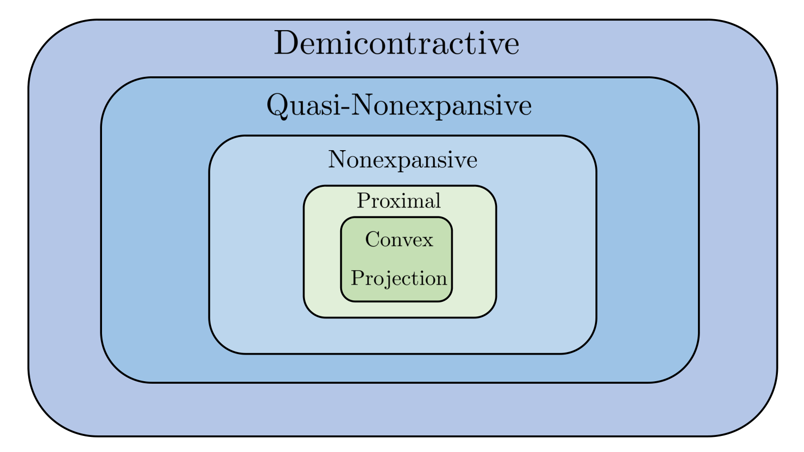
Notice that any Lipschitzian mapping admits a nonexpansive function by an appropriate scaling. In addition, as illustrated in Fig. 1, demicontractive mappings include the class of quasi-nonexpansive mappings, which in turn contains the widely studied class of nonexpansive operators. Thus, the class of demicontractive operators cover a large extent of functions and it is one of the most general classes for which some iterative methods were investigated [65], explaining their centrality in this work. Below we provide results concerning the structure of the fixed point set for demicontractive mappings.
Definition 6.
Consider a mapping and let . Then, the relaxation of is defined as the averaged operator where is the identity operator. Notice it holds that .
Proposition 7.
Consider a -demicontractive mapping and . Then, the relaxed operator is -strongly quasi-nonexpansive with .
Proof.
See section A.1.
proposition 7 provides us a simple tool to construct a strong quasi-nonexpansive map from a demicontractive mapping, which we utilize in the next section.
The following theorem is the foundation on which we shall base our problem formulation, introduced in Section 4.
Theorem 8 ([27, 27]).
Suppose that is a -demicontractive mapping. Then, the fixed-point set is closed and convex .
Proof.
See Lemma 5 of [27].
3.2 Demicontractive Denoisers
A fair and necessary question is whether general denoisers are demicontractive. While we cannot fully answer this question, we provide below supporting claims to our assumption of demicontractivity of the denoiser. We start with a typical assumption in convex optimization and gradually relax it to demicontractivity. Then, we directly relate the latter assumption to other common conditions for the convergence of PnP and RED.
Given a denoiser , we define the denoising residual as . The RED framework aims at showing that under certain assumption on , the residual is the gradient of an explicit convex function. Similarly, PnP can be seen an extension of Bayesian regularization [82] where the denoiser is a proximal operator of a (possibly implicit) function , which in turn implies that the residual is the gradient of the convex Moreau envelope of [70]. Therefore, by the Baillon-Haddad theorem [2, 6], if the residual is -Lipschitz continuous, it is -co-coercive
| (20) |
The notion of co-coercivity plays an important role in the convergence of iterative schemes [106]. However, for general denoisers we cannot assume that the residual is the gradient of some convex function. Fortunately, this condition can be relaxed as follows.
Proposition 9.
Assume the mapping is Lipschitz continuous with Lipschitz constant , then, is co-coercive.
Proof.
See [106] Proposition 2.3.
The latter proposition provides a condition for the co-coercivity of the residual regardless if it the gradient of the a convex function or not. We further relax our assumptions on the denoisers and require that eq. 20 hold only with respect to :
| (21) |
Substituting and noticing that , we observe that eq. 21 coincides with eq. 14 with . Thus, eq. 21 provide us an approximation of , assuming we have an estimation of the Lipschitz constant of the residual, and more importantly, shows that the assumption of demicontractive denoisers is broader than co-coercivity, allowing us to go beyond common optimization schemes.
We cannot conclude this part without discussing other previously-made assumptions and show their relation to demicontractivity. First, notice that any denoiser which meets conditions (C1)-(C4) is nonexpansive:
In [83], the authors prove that the RED algorithms converge when the denoiser is block-nonexpansive. In partiuclar, when the block is taken to be the entire image, it implies that the denoiser is nonexpansive. Various studies [82, 18, 84, 89, 88, 21, 74] have proven the convergence of variants of PnP for nonexpansive or averaged denoisers. Thus, all mentioned works assume demicontractive denoisers. Recently, the authors of [79] have shown that PnP-ADMM and PnP forward-backward splitting converge under weaker conditions where Lipschitz continuous mapping satisfying
| (22) |
for some small . Assuming , the above condition is relaxed to the following assumption
| (23) |
By the definition of demicontractivity (14) in conjunction with the Cauchy-Schwartz inequality we obtain that any -demicontractive function satisfies , which it turn implies that
| (24) |
Thus, it is clear that any -demicontractive function meets condition (23) with .
In [84], Chan et al. have proposed a version of PnP-ADMM for bounded denoisers
| (25) |
where they assume any point x is bounded in some interval (), is a parameter controlling the strength of the denoiser and is a constant independent of and . Bounded denoisers are asymptotically invariant in the sense that as . Under the boundedness assumption (25), a fixed-point convergence of the modified PnP-ADMM has been proven where a diminishing step size has been used and for some predefined .44 4 The original formulation in [84] defines an increasing penalty parameter which satisfies . However, this approach requires the denoiser to have an internal parameter controlling its strength which may not be available. We offer an external control which relies only on the demicontractivity of the denoiser, as given the in the following proposition.
Proposition 10.
Consider a -demicontractive denoiser and define the relaxed operator for some . Then, it holds that
| (26) |
where and .
Proof.
See section A.2
The above theorem provides the mean to externally control the strength of a denoiser by performing appropriate averaging. This is important by itself, since it may boost the performance of PnP methods [96]. Moreover, by updating at each iteration we obtain , which ensures the convergence of the PnP-ADMM presented in [84] for demicontractive denoisers.
Following the discussion above, while demicontractivity is hard to verify for general denoisers (as other conditions), we have shown that the condition of demicontractivity is covers a wide range of operators and is and broader than other common assumptions.
4 RED-PRO: RED via Fixed-Point Projection
As discussed in Section 2, the PnP and RED frameworks have achieved state-of-the-art performance in solving inverse problems by utilizing denoisers as regularization. However, their theoretical analysis is incomplete since it is unclear which objective functions are minimized by PnP and RED,55 5 We are referring to the case where the denoiser is non-differentiable or having a non-symmetric Jacobian. and whether such cost functions exist. As a partial answer, we consider in appendix B non-differentiable denoisers and we provide convergence guarantees for the RED algorithms. In this section we address the matter of the underlying objective function for PnP and RED. To that end, we reformulate RED as a convex minimization problem regularized using the fixed-point set of a demicontractive denoiser. We provide simple solutions for the proposed problem, similar to PnP-PGM and PnP-ADMM. As such, we offer a theoretical explanation for the PnP approach and establish its connection to RED. Finally, we relax our problem by considering broader and richer domains than the fixed-point set. These modifications offer larger flexibility, allowing for a broader group of denoisers to be applicable.
4.1 Regularization by Projection
The new framework we propose builds upon the fixed-point set of demicontractive denoisers as prior for general inverse problems. To motivate our regularization strategy, described later, we make the following observation:
Proposition 11.
Consider a demicontractive denoiser and assume . Then,
Proof.
It is clear that for any , we get . For the other direction, we recall that by the definition of demicontractive mapping for any
| (27) |
where we use the assumption that is a fixed-point. Therefore, when , then , implying that .
Inspired by this observation,66 6 The assumption is not necessary for our derivations but is only used to explain our motivation. we introduce the following general minimization problem, which is the main message of this paper:
| (28) | ||||
We refer to the above as the RED via Fixed-Point Projection (RED-PRO) paradigm, where we utilize the fixed-point set of a denoising engine as a regularization for our inverse problem. The optimization task (28) can be interpreted as searching for a minimizer of over the set of ”clean” images. Ideally, we would like to limit our search to the manifold of natural images [68, 91, 75]. However, the set is generally not well-defined, it is not easy accessible and it is not convex,77 7 The convex interpolation of two natural images may not be a natural image making the search within this domain difficult. Therefore, as an alternative, we propose to use which is well-behaved for demicontractive denoisers and should satisfy for a “perfect” denoiser. Note, however, that common denoisers are far from being ideal, hence, the solution of eq. 28 is sensitive to the choice of the denoiser and it may vary considerably for different choices, as shown in Section 5.
Surprisingly, although the constraint of eq. 28 is not linear in nature, the RED-PRO approach admits a convex optimization problem as stated by the next theorem.
Theorem 12.
Assume the denoiser is a -demicontractive mapping. Then, (28) defines a convex minimization problem.
Proof.
The above theorem allows to find solutions to eq. 28 and to derive convergence guarantees using tools from convex optimization. Moreover, as shown in section 3.1, it holds that for any where is the relaxed operator. Thus, we can rewrite (28) equivalently as
| (29) |
While the latter seems as an unnecessary and redundant step, it plays a crucial role in our convergence results since is strongly quasi-nonexpansive for an appropriate choice of . To find a solution for our proposed problem (28), one may apply the projected gradient descent method [71, 13] as follows
| (30) |
where is the gradient step size and denotes the projection onto the fixed-point set . The above update rule resembles other studies that aim at projecting onto the set of natural images (see e.g. [68, 91, 75]), however, we utilize which exhibits favorable properties for demicontractive denoisers. Furthermore, we offer here a simpler solution, based on the hybrid steepest descent method (HSD) [34, 99, 5, 98], which performs one activation of the denoising engine per iteration, as detailed in algorithm 3.
- •
- •
- •
We note that algorithm 3 can be written in a compact form as
| (31) |
The next theorems provide conditions for the convergence of algorithm 3 to an optimal solution of (28) where we distinguish between two cases: diminishing and constant step sizes.
Theorem 13 (Diminishing Step Size).
Let be a continuous -demicontractive denoiser and be a proper convex l.s.c differentiable function with L-Lipschitz gradient . Assume the following:
- (A1)
.
- (A2)
where and .
Then, the sequence generated by algorithm 3 converges to an optimal solution of the RED-PRO problem.
Proof.
See section A.3.
Theorem 14 (Constant Step Size).
Let be a continuous -demicontractive denoiser and is a proper convex l.s.c differentiable function with L-Lipschitz gradient . Assume the following:
- (H1)
.
- (H2)
.
- (H3)
where .
Then, the sequence generated by algorithm 3 converges an optimal solution of the RED-PRO problem.
Proof.
See section A.4.
theorem 13 and theorem 14 provide convergence guarantees of HSD to a solution of the RED-PRO formulation. Moreover, recalling eq. 31, algorithm 3 resembles the PnP-PGD method, suggesting that the above theorems may provide insights into the solutions of PnP-PGD. We establish this connection in the following subsection.
4.1.1 PnP and RED as a special case
PnP and RED can be seen as two alternative approaches for utilizing denoising engines as regularization for general inverse problems. Below, we aim at bridging PnP and RED via the RED-PRO framework, hopefully enriching the theoretical understanding of these two approaches and related ones.
Several variants of the RED algorithms have been proposed, see [83, 1, 74] to name just a few. In particular, the authors of [1] discussed an accelerated gradient descent version of RED with the following update rule
- •
,
- •
,
- •
,
where is an acceleration step size and is a design parameter. Thus, when we set , i.e. when we skip the acceleration step, the above RED variant reduces to the iterative update eq. 31. In addition, when we continue and set , we obtain the PnP-PGD method, showing that the three frameworks coincide under this setup. We note that under the assumptions of the RED-PRO framework, it is possible to set when the denoiser in use is strongly quasi-nonexpansive, rather than only demicontractive. Therefore, the RED-PRO framework provides an optimization interpretation to PnP-PGD above along with convergence results when the conditions of theorem 14 hold. However, eq. 28 as well as PnP-PGD may converge even when condition (H3) is not satisfied. In this case, algorithm 3 converges to a solution of a special case of the RED-PRO formulation, as stated by the next theorem.
Theorem 15.
Let be a continuous -demicontractive denoiser and is a proper convex l.s.c differentiable function whose gradient is L-Lipschitz. Assume the following holds
- (W1)
.
- (W2)
.
- (W3)
and where .
Then, the sequence generated by algorithm 3 converges an optimal solution of the following convex feasibility problem:
| (32) | ||||
i.e., find such that . .
Proof.
Under the assumption that , the mapping is an averaged quasi-nonexpansive operator as composition of averaged operators. Hence, is closed and convex and problem eq. 32 can be seen a special of the RED-PRO formulation with respect to the composed denoiser . Thus, the conditions of theorem 13 and theorem 14 hold and the iteration converges to an arbitrary fixed-point of .
Several remarks are to be made with regard to the above theoretical results. As discussed earlier, PnP-PGD can be seen a special case of algorithm 1 when the denoiser is strongly quasi-nonexpansive, hence, the above theorem complements theorem 14 with respect to the convergence of PnP-PGD. However, notice that unlike (H3), condition (W3) depends on . Consequently, the solution of (32) is sensitive to the choice of , which is consistent with previous observations in the literature on the convergence of PnP [93]. While the convergence of PnP-PGD (and other variants) to a fixed-point was studied and proven before, here, we first present it a solution of a convex optimization problem, establishing the connection between the PnP and RED-PRO frameworks. Furthermore, it has been shown [67, 84, 79] that other PnP variants, e.g., PnP-ADMM and PnP primal-dual hybrid gradient method (PnP-PDHG), satisfy the same fixed-point equation as PnP-PGM
| (33) |
Therefore, under the conditions stated above, any algorithm that converges to a fixed-point satisfying (33), leads in principle to a solution of the RED-PRO formulation. Examining the latter, we observe that in general the solution of eq. 32 is not unique and algorithm 3 converges to an arbitrary fixed-point. This may explain why while different versions of PnP share the same fixed-point equation eq. 33, they converge to different solutions. Thus, we can gain more control on the obtained solution by formulating the following problem
| (34) | ||||
for some desired , which can be solved by algorithm 3 with a diminishing step size, leading to . This allows, for example, to obtain the minimal norm solution that satisfies eq. 33 by setting .
4.2 Relaxed RED-PRO
So far, we have introduced the RED-PRO framework which utilizes the fixed-point set of a denoiser as a regularization, and we have shown its connection to both PnP and RED. However, as mentioned earlier, the fixed-point sets of practical denoisers might be narrow, leading to unfavorable recovery solutions. To circumvent this limitation, we here relax the hard constraint of eq. 28 and replace it with a squared distance penalty, leading to a relaxed RED-PRO minimization problem
| (35) |
As before, when the denoiser is demicontractive, the above problem is a well-defined convex minimization. Here balances between the log-likelihood term and the regularization, allowing us to control the distance of the optimal solution from the fixed-point set. Notice that when (or it sufficiently large), problem (35) reduces to problem (28).
Denoting by the objective function of (35), we have that
| (36) |
Note that the latter expression is similar to the gradient eq. 11 of the original RED framework, where we replace the denoiser with the projection onto its fixed-point set. Therefore, the solution of (35) can be found by various optimization solvers, such as SD and ADMM, assuming one can compute the projection onto the fixed-point set
| (37) |
Notice that the above problem is a special case of problem (28) where the objective is which satisfies the conditions of theorem 13. Therefore, given a point , we can compute the projection using the following iterative scheme
| (38) |
where and the sequence meet the requirements of theorem 13. As shown in section A.5, the above update rule can be rewritten equivalently as
| (39) |
The relaxed RED-PRO approach offers a broader search domain at the expense of higher computational load, since it require multiple activations of the denoising engine in each iteration. As typically done, we limit ourselves in practice to a small number of inner iterations to reduce complexity, yielding an approximation of the projection at each iteration.
As a side note, we mention that for demicontractive denoiser it holds that implying that is a descent direction of the regularization term . Hence, an interesting direction to reduce complexity is replacing the term in eq. 36 with g, bringing us back to the original RED algorithms. However, it remains unclear whether this indeed leads to a solution of eq. 35.
Next, we further relax our problem by considering richer sets than the fixed-point one. To that end, we define for the -approximate fixed-points as
| (40) |
Note that can be seen as the set of “almost clean” images, thus, it can act as a valid and wide domain for searching restored solutions. A possible approach to exploit is defining an adaptive averaged denoiser
| (41) |
where . Now notice that , hence, the modified denoiser (41) can be utilized via the algorithms derived earlier to find inverse solutions constrained by . While empirically this may lead to satisfactory results, the approximate fixed-point set is generally not convex for demicontractive or even nonexpansive functions. Consequently, the projection onto is not well-defined and no convergence guarantees can be given. One option standing ahead of us is to restrict the valid denoisers to those for which this set is necessarily convex.
Another option for circumventing the above difficulty is to consider a dilated fixed-point set, defined for some as
| (42) |
The set is closed and convex for any demicontractive denoiser. Moreover, as illustrated in Fig. 2, for an appropriate choice of we have that as stated next.
Theorem 16.
Let be -demicontractive function and consider for some and . Then, .
Proof.
See section A.6.

Exploiting the above result, we formulate the relaxed RED-PRO (RRP) problem
| (43) |
where is the projection onto . The gradient of the above objective is
| (44) |
requiring to compute the projection . Fortunately, for any , the projection is given by [3]
| (45) |
Substituting the above expression into eq. 43, we obtain
| (46) |
The latter minimization problem consists of another design parameter which allows to control the distance of the solution from the fixed-point set, thus, increasing our search domain. When is set to zero, we return to problem (35). In algorithm 4 we detail the overall solution of the relaxed RED-PRO with parameter using steepest descent as an example.
-
.
-
for do:
-
.
-
To summarize this part, we described here relaxed versions of the RED-PRO framework where we use the distance function as regularization and we extend our search to certain approximate fixed-points. This allows us to obtain stable inverse solutions even when the denoiser exhibits a limited fixed-point set.
5 Experiments
In this section we evaluate the performance of the proposed RED-PRO framework. AS the goal of this study is to bridge between RED and PnP and to provide theoretical justifications rather than achieving state-of-the-art results, we compare ourselves to the original RED approach alone, for the tasks of image deblurring and super-resolution. We follow the same line of experiments performed in [77], where we employ NLM and TNRD denoisers, rather than the median filter and TNRD. We use NLM to exemplify the application of the RED-PRO with denoisers that may be expansive for certain parameters. The TNRD denoiser, pretrained to remove WGN whose standard deviation equals 5,88 8 We use TNRD to address any arbitrary noise level by exploiting the relation is brought to demonstrate the full extent of the proposed framework.
For fair comparison, the parameters that are common to both RED and RED-PRO are set according to the values given in [77].99 9 For RED algorithms we use the code published by the authors of [77] at https://github.com/google/RED. Additional parameters of introduced by the RED-PRO framework are tuned manually to achieve higher peak signal to noise ratio (PSNR).
5.1 Convergence
As a start, we demonstrate the convergence of RED-PRO with the HSD method for various denoisers. To that end, we consider the task of uniform deblurring whose complete setup is detailed in the following subsection, with the exception of the relaxation parameter that we set here to .
We show the evolution of the relative error the fidelity term throughout the iterations in Fig. 3(a) we, while Fig. 3(b) displays a measure for the solution proximity to the fixed-point set over iterations. We observe that we obtain small relative errors in both measures, where rapid decline the fidelity term is seen for all denoisers, converging to different values as expected. In addition, for all of the denoisers, the solution converge to a fixed point, however, the rate of convergence varies for different denoiser where BM3D exhibits notably greater decrease than other denoisers.1010 10 Due to this dramatic decline of BM3D, it may seem that the errors of other denoisers are saturated. However, this is not the case, as their errors gradually decrease. We point out that there is a tradeoff between the rate of convergence of the fidelity term and that of the fixed-point errors, since in general large step sizes lead to large decrease in the fidelity term while decaying step sizes are required to ensue convergence to a fixed-point. Finally, we note that while these measures indeed demonstrate the convergence of the proposed approach, they might not accurately indicate the quality of the resultant images.
5.2 Image Deblurring
As done in [77], we carry out here the synthetic non-blind deblurring experiments first described in [38]. To that end, we perform the following process on the RGB images provided by the authors of [77]. Each image is convolved either with a uniform point spread function (PSF) or a 2D Gaussian function with a standard deviation of 1.6. Then, we contaminate the resulted blurred images with an additive WGN with . The inverse operation is performed by first converting the RGB image to YCbCr color-space, applying the deblurring technique only on the luminance channel and then converting the result back to RGB to obtain the final image. The complete details of the parameter values for the uniform deblurring case are given in table 1. For Gaussian deblurring we use the same values excluding and which we set to 4.1 and 0.01 respectively. Throughout all the experiments, we use a constant step size for the steepest descent methods, while for HSD we use a a diminishing step size .
table 2 and table 4 detail the recovery results of RED and RED-PRO algorithms when NLM is used, while table 3 and table 5 provides the results when TNRD is employed. We evaluate the performance of the different techniques using PSNR measure, where higher is better, computed on the luminance channel of the ground truth and the restored images. We note that we show the results only for a chosen subset of images, while the displayed average value is computed over the entire set of images.
As can be seen, when NLM is used within the discussed frameworks, the RED-PRO approach displays an apparent improvement, in particular for the case of uniform deblurring. When TNRD is incorporated, the relaxed RED-PRO framework still leads to enhanced results in comparison to RED, but the performance gap is small. Furthermore, we notice that SD-based methods require more iterations which is consistent with the observations given in [77]. We present visual evidence for the performance of RED-PRO in Fig. 4 and Fig. 5 for uniform and Gaussian blur kernels, respectively. These images support the previous results where RED-PRO offer an improvement over the RED framework when NLM is utilized. In the other case, both approaches achieve similar performance with a clear advantage for applying TNRD rather than employing NLM.
| Parameter | RED | RED-PRO | Approximate RED-PRO | |||||||
|---|---|---|---|---|---|---|---|---|---|---|
| FP | ADMM | SD | HSD | FP | ADMM | SD | FP | ADMM | SD | |
| 200 | 200 | 1500 | 400 | 200 | 200 | 1500 | 200 | 200 | 1500 | |
| 3.25 | 3.25 | 3.25 | 3.25 | 3.25 | 3.25 | 3.25 | 3.25 | 3.25 | 3.25 | |
| 0.02 | 0.02 | 0.02 | — | 0.02 | 0.02 | 0.02 | 0.02 | 0.02 | 0.02 | |
| — | 0.001 | — | — | — | 0.001 | — | — | 0.001 | — | |
| *CF | *CF | — | — | *CF | *CF | — | *CF | *CF | — | |
| — | 1 | — | — | — | 1 | — | — | 1 | — | |
| — | — | — | 0.035 | 1 | 1 | 1 | 1 | 1 | 1 | |
| — | — | — | — | 3 | 3 | 3 | 3 | 3 | 3 | |
| — | — | — | — | — | — | — | 0.0001 | 0.0001 | 0.0001 | |
*Closed-form using FFT
| RED | RED-PRO | Relaxed RED-PRO | Relaxed RED-PRO | |||||||
|---|---|---|---|---|---|---|---|---|---|---|
| FP | ADMM | SD | HSD | FP | ADMM | SD | FP | ADMM | SD | |
| Bike | 23.07 | 23.12 | 24.41 | 24.95 | 23.09 | 23.16 | 24.46 | 23.08 | 23.13 | 24.51 |
| Butterfly | 24.93 | 25.01 | 26.93 | 27.47 | 24.93 | 25.00 | 26.96 | 24.83 | 24.87 | 26.89 |
| Flower | 26.21 | 26.25 | 27.89 | 29.26 | 26.27 | 26.33 | 27.97 | 26.25 | 26.27 | 28.01 |
| Girl | 31.29 | 31.32 | 31.86 | 32.68 | 31.35 | 31.42 | 31.93 | 31.40 | 31.43 | 31.98 |
| Hat | 29.04 | 29.06 | 30.40 | 31.42 | 29.15 | 29.13 | 30.49 | 29.08 | 29.05 | 30.46 |
| Average | 26.84 | 26.88 | 28.34 | 29.40 | 26.89 | 26.93 | 28.40 | 26.83 | 26.86 | 28.40 |
| RED | RED-PRO | Relaxed RED-PRO | Relaxed RED-PRO | |||||||
|---|---|---|---|---|---|---|---|---|---|---|
| FP | ADMM | SD | HSD | FP | ADMM | SD | FP | ADMM | SD | |
| Bike | 26.10 | 26.09 | 25.95 | 24.95 | 26.21 | 26.20 | 26.05 | 26.48 | 26.47 | 26.28 |
| Butterfly | 30.41 | 30.40 | 30.20 | 27.24 | 30.48 | 30.47 | 30.24 | 30.64 | 30.63 | 30.35 |
| Flower | 30.18 | 30.18 | 30.13 | 29.38 | 30.26 | 30.26 | 30.21 | 30.46 | 30.46 | 30.39 |
| Girl | 33.11 | 33.11 | 33.10 | 32.99 | 33.14 | 33.14 | 33.13 | 33.19 | 33.19 | 33.19 |
| Hat | 32.16 | 32.16 | 32.15 | 31.55 | 32.17 | 32.18 | 32.17 | 32.25 | 32.25 | 32.24 |
| Average | 30.67 | 30.67 | 30.56 | 29.54 | 30.75 | 30.75 | 30.63 | 30.92 | 30.92 | 30.77 |

| RED | RED-PRO | Relaxed RED-PRO | Relaxed RED-PRO | |||||||
|---|---|---|---|---|---|---|---|---|---|---|
| FP | ADMM | SD | HSD | FP | ADMM | SD | FP | ADMM | SD | |
| Bike | 25.30 | 25.45 | 26.97 | 27.13 | 25.38 | 25.54 | 27.03 | 25.42 | 25.57 | 27.08 |
| Butterfly | 27.14 | 27.28 | 29.61 | 29.87 | 27.18 | 27.36 | 29.64 | 27.21 | 27.37 | 29.66 |
| Flower | 28.47 | 28.62 | 30.75 | 31.64 | 28.58 | 28.73 | 30.85 | 28.61 | 28.77 | 30.92 |
| Girl | 33.32 | 33.45 | 33.33 | 32.97 | 33.33 | 33.41 | 33.29 | 33.29 | 33.36 | 33.27 |
| Hat | 30.84 | 30.95 | 32.39 | 32.74 | 30.92 | 31.04 | 32.45 | 30.96 | 31.08 | 32.47 |
| Average | 29.16 | 29.30 | 30.88 | 31.21 | 29.24 | 29.38 | 30.93 | 29.25 | 29.39 | 30.95 |
| RED | RED-PRO | Relaxed RED-PRO | Relaxed RED-PRO | |||||||
|---|---|---|---|---|---|---|---|---|---|---|
| FP | ADMM | SD | HSD | FP | ADMM | SD | FP | ADMM | SD | |
| Bike | 27.90 | 27.90 | 27.88 | 27.36 | 27.95 | 27.94 | 27.92 | 28.02 | 28.02 | 28.00 |
| Butterfly | 31.66 | 31.66 | 31.57 | 30.55 | 31.65 | 31.64 | 31.54 | 31.66 | 31.65 | 31.52 |
| Flower | 32.05 | 32.05 | 32.05 | 31.81 | 32.05 | 32.05 | 32.04 | 32.08 | 32.08 | 32.07 |
| Girl | 34.44 | 34.44 | 34.10 | 33.23 | 34.40 | 34.40 | 34.00 | 34.38 | 34.38 | 33.88 |
| Hat | 33.29 | 33.29 | 33.30 | 33.07 | 33.25 | 33.25 | 33.26 | 33.26 | 33.26 | 33.27 |
| Average | 32.15 | 32.15 | 32.09 | 31.53 | 32.14 | 32.14 | 32.07 | 32.16 | 32.16 | 32.06 |

5.3 Super-Resolution
Similar to [77], we continue with super-resolution experiments where ground-truth high-resolution images are blurred with Gaussian kernel with standard deviation of 1.6, downsampled by a factor of three at each axis and finally they are corrupted by an additive WGN with . To restore the images from their low-resolution versions, we convert them to YCbCr color-space and perform super-resolution where the chorma channels are up-scaled by bicubic interpolation and the luminance channel is processed by the discussed algorithms. The results are then transformed back to RGB, yielding the final super-resolved images. The parameter values are given by table 1 excluding , and which are set to 3, 0.008 and 200 respectively.
We present the restoration results of the different variants of RED and RED-PRO frameworks when NLM and TNRD are used in table 6 and table 7 respectively. As observed, the RED-PRO approach leads to slightly better results than RED. This is visually supported by the recovered images shown in Fig. 6 where we compare our approach to naive bicubic interpolation in addition to RED. Both quantitative and qualitative results point out the clear advantage of using TNRD over NLM.
| RED | RED-PRO | Relaxed RED-PRO | Relaxed RED-PRO | |||||||
|---|---|---|---|---|---|---|---|---|---|---|
| FP | ADMM | SD | HSD | FP | ADMM | SD | FP | ADMM | SD | |
| Bike | 22.97 | 23.04 | 22.27 | 23.10 | 23.02 | 23.08 | 22.34 | 23.05 | 23.11 | 22.41 |
| Butterfly | 25.27 | 25.37 | 24.23 | 24.85 | 25.30 | 25.39 | 24.29 | 25.32 | 25.40 | 24.37 |
| Flower | 26.70 | 26.82 | 25.42 | 27.21 | 26.79 | 26.91 | 25.48 | 26.89 | 27.02 | 25.64 |
| Girl | 30.75 | 30.78 | 30.03 | 30.50 | 30.84 | 30.90 | 30.13 | 30.96 | 31.02 | 30.19 |
| Hat | 29.19 | 29.27 | 28.19 | 28.73 | 29.25 | 29.34 | 28.29 | 29.28 | 29.38 | 28.31 |
| Average | 26.98 | 27.06 | 26.08 | 26.94 | 27.05 | 27.13 | 26.15 | 27.11 | 27.20 | 26.21 |
| RED | RED-PRO | Relaxed RED-PRO | Relaxed RED-PRO | |||||||
|---|---|---|---|---|---|---|---|---|---|---|
| FP | ADMM | SD | HSD | FP | ADMM | SD | FP | ADMM | SD | |
| Bike | 23.97 | 23.96 | 24.04 | 23.22 | 24.00 | 23.98 | 24.06 | 24.03 | 24.01 | 24.09 |
| Butterfly | 27.26 | 27.22 | 27.37 | 24.95 | 27.23 | 27.19 | 27.37 | 27.11 | 27.06 | 27.32 |
| Flower | 28.24 | 28.24 | 28.23 | 27.11 | 28.26 | 28.26 | 28.25 | 28.30 | 28.30 | 28.28 |
| Girl | 32.08 | 32.08 | 32.08 | 29.93 | 32.09 | 32.09 | 32.08 | 32.05 | 32.06 | 32.05 |
| Hat | 30.35 | 30.35 | 30.36 | 28.21 | 30.37 | 30.36 | 30.37 | 30.36 | 30.35 | 30.37 |
| Average | 28.33 | 28.32 | 28.36 | 26.79 | 28.34 | 28.33 | 28.38 | 28.33 | 28.31 | 28.38 |

6 Conclusion
The massive advancement in image denoising has led in recent years to the development of PnP and RED frameworks, which leverage the power of denoisers to solve other challenging inverse problems. These approaches have shown remarkable performance, leading to state-of-the-art results in unsupervised tasks such as image deblurring and super-resolution. However, PnP lacks an underlying global objective function, while RED demands restrictive conditions that are not met by many popular denoisers.
In this paper, we address the above limitations. The main contribution of this work is the introduction of the RED-PRO framework, which relies on the fixed-point set of demicontractive denoisers. We formulate a general inverse problem that exploits the convexity of the fixed-point set and utilize it as a regularization. Then, we derive several iterative methods for solving the proposed problems and prove their convergence to global optimum. We discuss the relation of the presented framework to PnP and RED, including the connection of demicontractivity to popular assumptions. This shows that RED-PRO joins ideas from both PnP and RED, bridging between the two framework. Thus, RED-PRO provides flexibility in choosing the denoiser and is guaranteed to converge to stable solutions. Furthermore, we present relaxed variants of RED-PRO related to the approximated fixed-point set, which is a much broader domain but not convex in general. Therefore, an open research direction is to provide the conditions under which the latter set is convex and derive different means to exploit it as a regularization. Finally, we perform experiments in image deblurring and super-resolution to demonstrate the validity of the regularization strategy, showing competitive and even improved performance in comparison to the original RED framework.
We conclude this section by briefly discussing key questions for future research. This study relies on the condition that the denoiser is demicontractive. Currently, determining whether an arbitrary denoiser satisfies this condition remains an open challenge. Certainly, any nonexpansive denoiser is also demicontractive, yet, it is unclear how to verify the nonexpansiveness of a general function. Therefore, it is of utmost practical importance to derive an efficient technique for testing the demicontractivity of a given mapping. An alternative approach can be using learned mappings enforced to satisfy this condition. Similar concept is applied in the field of deep learning where neural networks are constrained by a given Lipschitz constant [45] to obtain regularization during training and robustness to adversarial attacks.
In addition, as in [77], the RED-PRO framework exploits denoisers that are designed for optimized distortion measure, such as PSNR. However, this might lead to a low perceptual quality of the resultant images [14]. Hence, an interesting research direction is the deployment of denoisers based on some perceptual loss. Employing such denoisers in the RED-PRO scheme might result in solutions that better address the perception-distortion tradeoff [14]. Finally, the family of demicontractive mappings covers a broad range of functions, hence, a promising study direction is incorporating within the RED-PRO framework powerful mechanisms, different from denoisers, which encapsulate prior knowledge on the unknown image.
Appendix A Proofs
A.1 Proof of proposition 7
Given arbitrary and , we have
From (14), we get
Note that , implying that
which completes the proof.
A.2 Proof of proposition 10
For any bounded pair of points , we have
In addition, by proposition 7 we obtain
Hence, we get
which completes the proof.
A.3 Proof of theorem 13
Theorem 5 of [98] proves the convergence of algorithm 3 to a point in
under the assumptions that (A2) holds, is quasi-nonexpansive quasi-shrinking mapping ([20], Definition 4.3) and is paramonotone over , i.e.,
| ([20], Definition 11) |
When (A1) is satisfied, then, is continuous and strongly quasi-nonexpansive, hence, it is quasi-shrinking (See [19], Corollary 4.2 and Proposition 4.4). Moreover, since is convex over the set , we have that paramonotone over (See [20], Lemma 12). Therefore, the conditions of Theorem 5 in [98] hold and the sequence is guaranteed to converge to an optimal solution of (28).
A.4 Proof of theorem 14
We start with the following lemma:
Lemma 17 (Proposition 1 [98]).
Let and be two strongly quasi-nonexpansive mappings with constants and respectively such that . Then, the composition is -strongly quasi-nonexpansive where and it satisfies .
By proposition 7, the mapping is strongly quasi-nonexpansive. In addition, for we have that is averaged nonexpansive operator (See [100], Remark 17.16), in particular it is strongly quasi-nonexpansive. Define , then by lemma 17, is continuous and -strongly quasi-nonexpansive for some with . Furthermore, we can rewrite algorithm 3 as . Thus, for any it holds that
Therefore, the sequence is Fejér monotone w.r.t and is bounded. Moreover, we can rewrite the above inequality as
. Summing the above inequality for we get that
Thus, is a Cauchy sequence and for some . Since and , we have which in turn implies that and , completing the proof.
A.5 Proof of
The update rule for computing the projection onto the fixed-point set is
| (47) |
This can be rewritten in two stages as
Hence, we can rewrite the update rule with respect to as
Finally, by interchanging the roles of and we obtain eq. 39.
A.6 Proof of Theorem 16
Consider and define the averaged operator . By proposition 7, is -strongly quasi-nonexpansive with . Hence, according to proposition 3 we have . In addition, it holds that
Therefore, for any where , we have
which implies that .
Appendix B RED Revisited
Here, we complement the work in [74] by considering the RED framework and studying the case in which the denoiser is non-differentiable. We do so by reformulating the RED optimization problem using the Rockafellar function [76]. To make this part as self-contained as possible, we first recall essential results from variational analysis [76].
Definition 18.
A continuous mapping is maximal cyclically monotone if for every set of points in and any it holds that
Definition 19.
We say is cyclically firmly nonexpansive if for every set of points in and any it holds that
The following proposition connects cyclically firmly nonexpansive mappings with cyclically maximal monotone operators. This relationship shall allow us to establish the convergence of RED algorithms.
Proposition 20 ([8]).
Let be cyclically firmly nonexpansive and consider the displacement mapping . Then, is maximal cyclically monotone.
Now, we define the Rockafellar function which we shall use regularization.
Definition 21 (Rockafellar function [76]).
Consider a mapping and let be an arbitrary point. For , we define the following function with parameter u
where . Then, the Rockafellar function is defined as
The Rockafellar function in a well-known and important function in the area of variational analysis [4], which exhibits favorable properties when is maximal cyclically monotone as stated below.
Proposition 22 (Fact 3.2, [4]).
Let be maximal cyclically monotone and let . Then, is convex, l.s.c, proper function with and for any
Moreover, for any convex, l.s.c and proper function for which , it holds that , i.e., is uniquely determined by up to an additive constant.
Equipped with the above results, we formulate the next inverse problem. Let be a continuous denoiser and define the denoiser residual . For arbitrary and , we consider the following minimization problem
| (48) |
When the denoiser is cyclically firmly nonexpansive, the above formulation admits convex minimization problem which can be solved by the RED algorithms presented in [77], as proven in the next theorem.
Theorem 23.
Proof.
By proposition 20 in conjunction with proposition 22, the residual mapping is maximal cyclically monotone, hence, is a convex differentiable function whose gradient is . The latter in turn implies that
To conclude, theorem 23 provides the condition under which the RED approach minimizes a convex minimization problem given by (48), and thus it proves the convergence of RED algorithms. This holds even for the case where the denoiser is not differentiable. We note that the requirement of to be maximal cyclically monotone is a necessary condition, whereas the demand of to be cyclically firmly nonexpansive is a sufficient condition that might be relaxed and is fulfilled by e.g. proximal operators.
References
- [1] R. Ahmad, C. A. Bouman, G. T. Buzzard, S. Chan, S. Liu, E. T. Reehorst, and P. Schniter, Plug-and-play methods for magnetic resonance imaging: Using denoisers for image recovery, IEEE Signal Processing Magazine, 37 (2020), pp. 105–116.
- [2] J.-B. Baillon and G. Haddad, Quelques propriétés des opérateurs angle-bornés etn-cycliquement monotones, Israel Journal of Mathematics, 26 (1977), pp. 137–150.
- [3] C. Bargetz, S. Reich, and R. Zalas, Convergence properties of dynamic string-averaging projection methods in the presence of perturbations, Numerical Algorithms, 77 (2018), pp. 185–209.
- [4] S. Bartz, H. H. Bauschke, J. M. Borwein, S. Reich, and X. Wang, Fitzpatrick functions, cyclic monotonicity and Rockafellar’s antiderivative, Nonlinear Analysis: Theory, Methods & Applications, 66 (2007), pp. 1198–1223.
- [5] H. H. Bauschke, R. S. Burachik, P. L. Combettes, V. Elser, D. R. Luke, and H. Wolkowicz, Fixed-point algorithms for inverse problems in science and engineering, vol. 49, Springer Science & Business Media, 2011.
- [6] H. H. Bauschke and P. L. Combettes, The Baillon-Haddad theorem revisited, Journal of Convex Analysis, 17 (2010), pp. 781–787.
- [7] H. H. Bauschke, P. L. Combettes, et al., Convex analysis and monotone operator theory in Hilbert spaces, vol. 408, Springer, 2011.
- [8] H. H. Bauschke, S. M. Moffat, and X. Wang, Firmly nonexpansive mappings and maximally monotone operators: correspondence and duality, Set-Valued and Variational Analysis, 20 (2012), pp. 131–153.
- [9] M. Bayati and A. Montanari, The dynamics of message passing on dense graphs, with applications to compressed sensing, IEEE Transactions on Information Theory, 57 (2011), pp. 764–785.
- [10] A. Beck, First-order methods in optimization, vol. 25, SIAM, 2017.
- [11] A. Beck and M. Teboulle, Fast gradient-based algorithms for constrained total variation image denoising and deblurring problems, IEEE Transactions on image processing, 18 (2009), pp. 2419–2434.
- [12] R. Berthier, A. Montanari, and P.-M. Nguyen, State evolution for approximate message passing with non-separable functions, Information and Inference: A Journal of the IMA, 9 (2020), pp. 33–79.
- [13] D. P. Bertsekas, Nonlinear programming, Journal of the Operational Research Society, 48 (1997), pp. 334–334.
- [14] Y. Blau and T. Michaeli, The perception-distortion tradeoff, in Proceedings of the IEEE CVPR, 2018, pp. 6228–6237.
- [15] A. M. Bruckstein, D. L. Donoho, and M. Elad, From sparse solutions of systems of equations to sparse modeling of signals and images, SIAM review, 51 (2009), pp. 34–81.
- [16] A. Buades, B. Coll, and J.-M. Morel, A non-local algorithm for image denoising, in IEEE CVPR, vol. 2, 2005, pp. 60–65.
- [17] H. C. Burger, C. J. Schuler, and S. Harmeling, Image denoising: Can plain neural networks compete with BM3D?, in IEEE CVPR, 2012, pp. 2392–2399.
- [18] G. T. Buzzard, S. H. Chan, S. Sreehari, and C. A. Bouman, Plug-and-play unplugged: Optimization-free reconstruction using consensus equilibrium, SIAM Journal on Imaging Sciences, 11 (2018), pp. 2001–2020.
- [19] A. Cegielski and R. Zalas, Properties of a class of approximately shrinking operators and their applications, Fixed Point Theory, 15 (2014), pp. 399–426.
- [20] Y. Censor, A. N. Iusem, and S. A. Zenios, An interior point method with Bregman functions for the variational inequality problem with paramonotone operators, Mathematical Programming, 81 (1998), pp. 373–400.
- [21] S. H. Chan, Performance analysis of plug-and-play admm: A graph signal processing perspective, IEEE Transactions on Computational Imaging, 5 (2019), pp. 274–286.
- [22] S. H. Chan, X. Wang, and O. A. Elgendy, Plug-and-play ADMM for image restoration: Fixed-point convergence and applications, IEEE Transactions on Computational Imaging, 3 (2016), pp. 84–98.
- [23] P. Chatterjee and P. Milanfar, Is denoising dead?, IEEE Transactions on Image Processing, 19 (2009), pp. 895–911.
- [24] P. Chatterjee and P. Milanfar, Patch-based near-optimal image denoising, IEEE Transactions on Image Processing, 21 (2011), pp. 1635–1649.
- [25] Y. Chen and T. Pock, Trainable nonlinear reaction diffusion: A flexible framework for fast and effective image restoration, IEEE Transactions on Pattern Analysis and Machine Intelligence, 39 (2016), pp. 1256–1272.
- [26] T. Chernyakova, R. Cohen, R. Mulayoff, Y. Sde-Chen, C. Fraschini, J. Bercoff, and Y. C. Eldar, Fourier-domain beamforming and structure-based reconstruction for plane-wave imaging, IEEE Transactions on Ultrasonics, Ferroelectrics, and Frequency Control, 65 (2018), pp. 1810–1821.
- [27] C. E. Chidume and Ş. Măruşter, Iterative methods for the computation of fixed points of demicontractive mappings, Journal of Computational and Applied Mathematics, 234 (2010), pp. 861–882.
- [28] R. Cohen and Y. C. Eldar, Optimized sparse array design based on the sum coarray, in IEEE International Conference on Acoustics, Speech and Signal Processing (ICASSP), 2018, pp. 3340–3343.
- [29] R. Cohen and Y. C. Eldar, Sparse convolutional beamforming for ultrasound imaging, IEEE Transactions on Ultrasonics, Ferroelectrics, and Frequency Control, 65 (2018), pp. 2390–2406.
- [30] R. Cohen and Y. C. Eldar, Sparse Doppler sensing based on nested arrays, IEEE Transactions on Ultrasonics, Ferroelectrics, and Frequency Control, 65 (2018), pp. 2349–2364.
- [31] R. Cohen, Y. Zhang, O. Solomon, D. Toberman, L. Taieb, R. J. van Sloun, and Y. C. Eldar, Deep convolutional robust PCA with application to ultrasound imaging, in IEEE International Conference on Acoustics, Speech and Signal Processing (ICASSP), 2019, pp. 3212–3216.
- [32] K. Dabov, A. Foi, V. Katkovnik, and K. Egiazarian, Image denoising by sparse 3-D transform-domain collaborative filtering, IEEE Transactions on image processing, 16 (2007), pp. 2080–2095.
- [33] A. Danielyan, V. Katkovnik, and K. Egiazarian, Image deblurring by augmented lagrangian with bm3d frame prior, in Workshop on Information Theoretic Methods in Science and Engineering (WITMSE), Tampere, Finland, 2010, pp. 16–18.
- [34] F. Deutsch and I. Yamada, Minimizing certain convex functions over the intersection of the fixed point sets of nonexpansive mappings, Numerical Functional Analysis and Optimization, 19 (1998), pp. 33–56.
- [35] W. Dong, X. Li, L. Zhang, and G. Shi, Sparsity-based image denoising via dictionary learning and structural clustering, in CVPR 2011, 2011, pp. 457–464.
- [36] W. Dong, G. Shi, Y. Ma, and X. Li, Image restoration via simultaneous sparse coding: Where structured sparsity meets Gaussian scale mixture, International Journal of Computer Vision, 114 (2015), pp. 217–232.
- [37] W. Dong, P. Wang, W. Yin, G. Shi, F. Wu, and X. Lu, Denoising prior driven deep neural network for image restoration, IEEE Transactions on Pattern Analysis and Machine Intelligence, 41 (2018), pp. 2305–2318.
- [38] W. Dong, L. Zhang, G. Shi, and X. Li, Nonlocally centralized sparse representation for image restoration, IEEE Transactions on Image Processing, 22 (2012), pp. 1620–1630.
- [39] D. L. Donoho, A. Maleki, and A. Montanari, Message-passing algorithms for compressed sensing, Proceedings of the National Academy of Sciences, 106 (2009), pp. 18914–18919.
- [40] K. Egiazarian and V. Katkovnik, Single image super-resolution via BM3D sparse coding, in IEEE European Signal Processing Conference (EUSIPCO), 2015, pp. 2849–2853.
- [41] M. Elad, Sparse and redundant representations: from theory to applications in signal and image processing, Springer Science & Business Media, 2010.
- [42] M. Elad and M. Aharon, Image denoising via sparse and redundant representations over learned dictionaries, IEEE Transactions on Image processing, 15 (2006), pp. 3736–3745.
- [43] A. K. Fletcher, P. Pandit, S. Rangan, S. Sarkar, and P. Schniter, Plug-in estimation in high-dimensional linear inverse problems: A rigorous analysis, in Advances in Neural Information Processing Systems, 2018, pp. 7440–7449.
- [44] G. H. Golub, P. C. Hansen, and D. P. O’Leary, Tikhonov regularization and total least squares, SIAM Journal on Matrix Analysis and Applications, 21 (1999), pp. 185–194.
- [45] H. Gouk, E. Frank, B. Pfahringer, and M. Cree, Regularisation of neural networks by enforcing Lipschitz continuity, arXiv preprint arXiv:1804.04368, (2018).
- [46] R. Gribonval, Should penalized least squares regression be interpreted as maximum a posteriori estimation?, IEEE Transactions on Signal Processing, 59 (2011), pp. 2405–2410.
- [47] R. Gribonval and M. Nikolova, On Bayesian estimation and proximity operators, Applied and Computational Harmonic Analysis, (2019).
- [48] R. Gribonval and M. Nikolova, A characterization of proximity operators, Journal of Mathematical Imaging and Vision, 62 (2020), pp. 773–789.
- [49] S. Gu, L. Zhang, W. Zuo, and X. Feng, Weighted nuclear norm minimization with application to image denoising, in IEEE CVPR, 2014, pp. 2862–2869.
- [50] S. Guo, Z. Yan, K. Zhang, W. Zuo, and L. Zhang, Toward convolutional blind denoising of real photographs, in Proceedings of the IEEE Conference on Computer Vision and Pattern Recognition, 2019, pp. 1712–1722.
- [51] B. Halpern, Fixed points of nonexpanding maps, Bulletin of the American Mathematical Society, 73 (1967), pp. 957–961.
- [52] T. Hong, Y. Romano, and M. Elad, Acceleration of RED via vector extrapolation, Journal of Visual Communication and Image Representation, 63 (2019), p. 102575.
- [53] U. S. Kamilov, H. Mansour, and B. Wohlberg, A plug-and-play priors approach for solving nonlinear imaging inverse problems, IEEE Signal Processing Letters, 24 (2017), pp. 1872–1876.
- [54] C. Knaus and M. Zwicker, Dual-domain image denoising, in IEEE International Conference on Image Processing, 2013, pp. 440–444.
- [55] A. Krull, T.-O. Buchholz, and F. Jug, Noise2void-learning denoising from single noisy images, in Proceedings of the IEEE Conference on Computer Vision and Pattern Recognition, 2019, pp. 2129–2137.
- [56] R. L. Lagendijk and J. Biemond, Basic methods for image restoration and identification, in The Essential Guide to Image Processing, Elsevier, 2009, pp. 323–348.
- [57] M. Lebrun, A. Buades, and J.-M. Morel, Implementation of the non-local Bayes (NL-Bayes) image denoising algorithm, Image Processing On Line, 3 (2013), pp. 1–42.
- [58] M. Lebrun, M. Colom, A. Buades, and J.-M. Morel, Secrets of image denoising cuisine, Acta Numerica, 21 (2012), pp. 475–576.
- [59] A. Levin and B. Nadler, Natural image denoising: Optimality and inherent bounds, in IEEE CVPR, 2011, pp. 2833–2840.
- [60] A. Levin, B. Nadler, F. Durand, and W. T. Freeman, Patch complexity, finite pixel correlations and optimal denoising, in European Conference on Computer Vision, Springer, 2012, pp. 73–86.
- [61] F. Lieder, On the convergence rate of the Halpern-iteration, Optimization Online preprint, (2017), pp. 11–6336.
- [62] B. Luijten, R. Cohen, F. J. De Bruijn, H. A. Schmeitz, M. Mischi, Y. C. Eldar, and R. J. Van Sloun, Adaptive ultrasound beamforming using deep learning, IEEE Transactions on Medical Imaging, (2020).
- [63] J. Mairal, F. Bach, J. Ponce, G. Sapiro, and A. Zisserman, Non-local sparse models for image restoration, in IEEE 12th international conference on computer vision, 2009, pp. 2272–2279.
- [64] S. Mallat, A wavelet tour of signal processing, Elsevier, 1999.
- [65] L. Măruşter and Ş. Măruşter, Strong convergence of the Mann iteration for -demicontractive mappings, Mathematical and Computer Modelling, 54 (2011), pp. 2486–2492.
- [66] G. Mataev, P. Milanfar, and M. Elad, DeepRED: Deep image prior powered by RED, in Proceedings of the IEEE International Conference on Computer Vision Workshops, 2019, pp. 0–0.
- [67] T. Meinhardt, M. Moller, C. Hazirbas, and D. Cremers, Learning proximal operators: Using denoising networks for regularizing inverse imaging problems, in Proceedings of the IEEE International Conference on Computer Vision, 2017, pp. 1781–1790.
- [68] S. Menon, A. Damian, S. Hu, N. Ravi, and C. Rudin, Pulse: Self-supervised photo upsampling via latent space exploration of generative models, in Proceedings of the IEEE/CVF Conference on Computer Vision and Pattern Recognition, 2020, pp. 2437–2445.
- [69] C. A. Metzler, A. Maleki, and R. G. Baraniuk, From denoising to compressed sensing, IEEE Transactions on Information Theory, 62 (2016), pp. 5117–5144.
- [70] J.-J. Moreau, Proximité et dualité dans un espace hilbertien, Bulletin de la Société mathématique de France, 93 (1965), pp. 273–299.
- [71] N. Parikh, S. Boyd, et al., Proximal algorithms, Foundations and Trends® in Optimization, 1 (2014), pp. 127–239.
- [72] A. Perelli and M. S. Andersen, Regularized Newton sketch by denoising score matching for computed tomography reconstruction, in Workshop on Signal Processing with Adaptive Sparse Structured Representations, 2019.
- [73] N. Pierazzo, M. E. Rais, J.-M. Morel, and G. Facciolo, Da3d: Fast and data adaptive dual domain denoising, in IEEE International Conference on Image Processing (ICIP), 2015, pp. 432–436.
- [74] E. T. Reehorst and P. Schniter, Regularization by denoising: Clarifications and new interpretations, IEEE Transactions on computational imaging, 5 (2018), pp. 52–67.
- [75] J. Rick Chang, C.-L. Li, B. Poczos, B. Vijaya Kumar, and A. C. Sankaranarayanan, One network to solve them all: Solving linear inverse problems using deep projection models, in Proceedings of the IEEE International Conference on Computer Vision, 2017, pp. 5888–5897.
- [76] R. T. Rockafellar and R. J.-B. Wets, Variational analysis, vol. 317, Springer Science & Business Media, 2009.
- [77] Y. Romano, M. Elad, and P. Milanfar, The little engine that could: Regularization by denoising (RED), SIAM Journal on Imaging Sciences, 10 (2017), pp. 1804–1844.
- [78] L. I. Rudin, S. Osher, and E. Fatemi, Nonlinear total variation based noise removal algorithms, Physica D: nonlinear phenomena, 60 (1992), pp. 259–268.
- [79] E. K. Ryu, J. Liu, S. Wang, X. Chen, Z. Wang, and W. Yin, Plug-and-play methods provably converge with properly trained denoisers, arXiv preprint arXiv:1905.05406, (2019).
- [80] M. Scetbon, M. Elad, and P. Milanfar, Deep K-SVD denoising, arXiv preprint arXiv:1909.13164, (2019).
- [81] O. Solomon, R. Cohen, Y. Zhang, Y. Yang, Q. He, J. Luo, R. J. van Sloun, and Y. C. Eldar, Deep unfolded robust PCA with application to clutter suppression in ultrasound, IEEE Transactions on Medical imaging, 39 (2019), pp. 1051–1063.
- [82] S. Sreehari, S. V. Venkatakrishnan, B. Wohlberg, G. T. Buzzard, L. F. Drummy, J. P. Simmons, and C. A. Bouman, Plug-and-play priors for bright field electron tomography and sparse interpolation, IEEE Transactions on Computational Imaging, 2 (2016), pp. 408–423.
- [83] Y. Sun, J. Liu, and U. Kamilov, Block coordinate regularization by denoising, in Advances in Neural Information Processing Systems, 2019, pp. 380–390.
- [84] Y. Sun, B. Wohlberg, and U. S. Kamilov, An online plug-and-play algorithm for regularized image reconstruction, IEEE Transactions on Computational Imaging, 5 (2019), pp. 395–408.
- [85] H. Takeda, S. Farsiu, and P. Milanfar, Kernel regression for image processing and reconstruction, IEEE Transactions on image processing, 16 (2007), pp. 349–366.
- [86] H. Talebi and P. Milanfar, Global image denoising, IEEE Transactions on Image Processing, 23 (2013), pp. 755–768.
- [87] T. Tasdizen, Principal neighborhood dictionaries for nonlocal means image denoising, IEEE Transactions on Image Processing, 18 (2009), pp. 2649–2660.
- [88] A. M. Teodoro, J. M. Bioucas-Dias, and M. A. Figueiredo, Scene-adapted plug-and-play algorithm with convergence guarantees, in IEEE 27th International Workshop on Machine Learning for Signal Processing (MLSP), 2017, pp. 1–6.
- [89] A. M. Teodoro, J. M. Bioucas-Dias, and M. A. Figueiredo, A convergent image fusion algorithm using scene-adapted Gaussian-mixture-based denoising, IEEE Transactions on Image Processing, 28 (2018), pp. 451–463.
- [90] T. Tirer and R. Giryes, Image restoration by iterative denoising and backward projections, IEEE Transactions on Image Processing, 28 (2018), pp. 1220–1234.
- [91] D. Ulyanov, A. Vedaldi, and V. Lempitsky, Deep image prior, in Proceedings of the IEEE CVPR, 2018, pp. 9446–9454.
- [92] S. V. Venkatakrishnan, C. A. Bouman, and B. Wohlberg, Plug-and-play priors for model based reconstruction, in IEEE Global Conference on Signal and Information Processing, 2013, pp. 945–948.
- [93] K. Wei, A. Aviles-Rivero, J. Liang, Y. Fu, C.-B. Schnlieb, and H. Huang, Tuning-free plug-and-play proximal algorithm for inverse imaging problems, in ” in Proc. 37th Int. Conf. Machine Learning (ICML), arXiv:2002.09611, 2020.
- [94] Z. Wu, Y. Sun, J. Liu, and U. Kamilov, Online regularization by denoising with applications to phase retrieval, in Proceedings of the IEEE International Conference on Computer Vision Workshops, 2019, pp. 0–0.
- [95] J. Xing, U. Kamilov, W. Wu, Y. Wang, and M. Zhang, Plug-and-play priors for reconstruction-based placental image registration, in Smart Ultrasound Imaging and Perinatal, Preterm and Paediatric Image Analysis, Springer, 2019, pp. 133–142.
- [96] X. Xu, J. Liu, Y. Sun, B. Wohlberg, and U. S. Kamilov, Boosting the performance of Plug-and-Play Priors via denoiser scaling, arXiv preprint arXiv:2002.11546, (2020).
- [97] X. Xu, Y. Sun, J. Liu, B. Wohlberg, and U. S. Kamilov, Provable convergence of plug-and-play priors with MMSE denoisers, arXiv preprint arXiv:2005.07685, (2020).
- [98] I. YAMADA, Hybrid steepest descent method for variational inequality problem over the fixed point set of certain quasi-nonexpansive mappings, Numerical Functional Analysis and Optimization, 25 (2004), pp. 619–655.
- [99] I. Yamada, N. Ogura, and K. Sakaniwa, Quadratic optimization of fixed points of nonexpansive mappings in Hilbert space, Numerical Functional Analysis and Optimization, 19 (1998), pp. 165–190.
- [100] I. Yamada, M. Yukawa, and M. Yamagishi, Minimizing the moreau envelope of nonsmooth convex functions over the fixed point set of certain quasi-nonexpansive mappings, in Fixed-Point Algorithms for Inverse Problems in Science and Engineering, Springer, 2011, pp. 345–390.
- [101] G. Yu, G. Sapiro, and S. Mallat, Solving inverse problems with piecewise linear estimators: From Gaussian mixture models to structured sparsity, IEEE Transactions on Image Processing, 21 (2011), pp. 2481–2499.
- [102] K. Zhang, W. Zuo, Y. Chen, D. Meng, and L. Zhang, Beyond a Gaussian denoiser: Residual learning of deep CNN for image denoising, IEEE Transactions on Image Processing, 26 (2017), pp. 3142–3155.
- [103] K. Zhang, W. Zuo, S. Gu, and L. Zhang, Learning deep CNN denoiser prior for image restoration, in Proceedings of the IEEE CVPR, 2017, pp. 3929–3938.
- [104] K. Zhang, W. Zuo, and L. Zhang, FFDNet: Toward a fast and flexible solution for CNN-based image denoising, IEEE Transactions on Image Processing, 27 (2018), pp. 4608–4622.
- [105] K. Zhang, W. Zuo, and L. Zhang, Deep plug-and-play super-resolution for arbitrary blur kernels, in Proceedings of the IEEE Conference on Computer Vision and Pattern Recognition, 2019, pp. 1671–1681.
- [106] D. L. Zhu and P. Marcotte, Co-coercivity and its role in the convergence of iterative schemes for solving variational inequalities, SIAM Journal on Optimization, 6 (1996), pp. 714–726.
- [107] D. Zoran and Y. Weiss, From learning models of natural image patches to whole image restoration, in IEEE International Conference on Computer Vision, 2011, pp. 479–486.