Faster Schrödinger-style simulation of quantum circuitsConference: ; ;
Abstract.
Recent demonstrations of superconducting quantum computers by Google and IBM and trapped-ion computers from IonQ fueled new research in quantum algorithms, compilation into quantum circuits, and empirical algorithmics. While online access to quantum hardware remains too limited to meet the demand, simulating quantum circuits on conventional computers satisfies many needs. We advance Schrödinger-style simulation of quantum circuits that is useful standalone and as a building block in layered simulation algorithms, both cases are illustrated in our results. Our algorithmic contributions show how to simulate multiple quantum gates at once, how to avoid floating-point multiplies, how to best use data-level and thread-level parallelism as well as CPU cache, and how to leverage these optimizations by reordering circuit gates. While not described previously, these techniques implemented by us supported published high-performance distributed simulations up to 64 qubits. To show additional impact, we benchmark our simulator against Microsoft, IBM and Google simulators on hard circuits from Google.
1. Introduction
Quantum computation was first developed theoretically to accelerate computational bottlenecks using quantum-mechanical phenomena (NC). Among several promising quantum models of computation, quantum circuits have been implemented in several technologies, for which end-to-end programmable computation has been demonstrated at intermediate scale (Preskill). In 2019, Google claimed quantum-computational supremacy (GoogleSuprem; Arute2019) by scaling quantum computation to the point where simulating it becomes exceptionally challenging even on supercomputers. The significance of quantum design automation tools has been appreciated for many years, to the point where IBM and Microsoft have developed extensive toolchains (QISKit and QDK respectively), which include language support, compilation, optimization, and a variety of execution back-ends for physical quantum computers and circuit simulators. Just like in conventional Electronic Design Automation, such software allows one to validate prototype designs before building the hardware.
Quantum circuit simulation in general is inherently difficult due to the exponential growth in the number of internal parameters and complexity-theoretic reasons (aaronson2016complexity; bouland_quantum_2018). We distinguish several categories and uses of quantum-circuit simulation:
- (1)
Polynomial-time simulation of "easy" special-case quantum circuits — those using Clifford gates (AG_2004), many instances of Grover’s algorithm (Viamontes), and circuits with small tree-width (TNC2008). Such simulation is used () to rule out quantum speed-up in specific algorithms, and () for limited initial testing of quantum computers in the lab and debugging of failed tests.
- (2)
Best-effort simulation of unrestricted "small" quantum circuits up to 40 qubits, as in Section 6, and also error modeling. Such simulation is used () for broad testing and routine debugging of quantum computers, () to verify local quantum circuit transformations and whole circuits, as well as () to evaluate new quantum algorithms, quantum error-correcting codes and device architectures (QS_opportunities). In particular, VQE algorithms common for quantum-chemistry applications run numerous quantum circuits in a sequence, their development particularly benefits from fast simulation (quantumChemistry_2020).
- (3)
Distributed quantum-circuit simulation on clusters and supercomputers (de_raedt_massively_2007; de_raedt_massively_2018; PB; qHIPSTER; IBM2017breaking; IBM2019storage; Villalonga_2020), including the world’s largest (Taihu). Such expensive and scarce resources are used to verify quantum computation and set performance baselines when claiming quantum-computational supremacy (GoogleSuprem; Arute2019; Villalonga_2020). Whereas other uses entail repeated on-demand simulations on readily available computing hardware, this category targets a small number of "expensive" one-off simulations.
All three categories of quantum-circuit simulation are in demand today, but high-performance simulation of unrestricted quantum circuits in Categories 2 and 3 is challenging and motivates algorithmic improvements of the type we propose. Using fast simulation to evaluate, verify, test and debug larger quantum circuits and algorithms facilitates the development of many applications.
Schrödinger-style simulation is the mainstream technique for general-case simulation of quantum algorithms, circuits and physical devices. It represents a quantum state (wave function) by a vector of complex-valued amplitudes and modifies this vector in place by applying quantum transformations (quantum gates, laser pulses, algorithmic modules, etc). Schrödinger simulation
- •
scales linearly with computation (circuit) depth but exponentially with the number of qubits, or width (Section 6.4);
- •
is commonly used for small and mid-size quantum-circuit and device/technology simulations because its unoptimized variants are relatively straightforward to implement;
- •
dominates supercomputer-based quantum circuit simulations because it can leverage distributed memory, fast interconnect, GPUs, etc (de_raedt_massively_2007; wecker2014liquid; de_raedt_massively_2018; PB; qHIPSTER; IBM2017breaking; Taihu; IBM2019storage);
- •
has been extended for better scalability via layered simulation (rr2020; teleport2020; IBM2019storage). For example, combining Schrödinger simulation with Feynman path summation enables scaling tradeoffs between circuit depth and width (aaronson2016complexity) and orders-of-magnitude resource savings in important cases (rr2020).
Our work accelerates both pure Schrödinger simulation and layered algorithms that use it, as we illustrate empirically for Schrödinger-Feynman simulation from (rr2020). Our algorithmic insights and innovations offer both constant-time implementation speed-ups and algorithmic speed-ups that scale with qubit count:
- •
Numerical accuracy improvements and checks to enable a compact floating-point data type which reduces memory footprint and bandwidth, and facilitates SIMD instructions.
- •
Avoiding most floating-point multiplications in favor of faster additive and bitwise instructions.
- •
Batched simulation of diagonal quantum gates that significantly reduces expensive memory traversals and the overall runtime while exposing thread-level parallelism.
- •
Encoding sets of same-type diagonal gates by bitmasks (Figure 6), simulating them with bitwise and mod- CPU instructions, and speeding up simulation with Gray codes.
- •
Encoding sets of same-type single-qubit (not necessarily diagonal) gates by bitmasks (Figure 8) and simulating them using a recursive FFT-like algorithm that improves cache locality and exposes thread-level parallelism.
- •
The insight that some quantum gates (implemented in superconducting quantum computers) are easier to simulate in pairs because this simplifies matrix elements and benefits from batched load/store operations.
- •
Gate clustering by type, contrasted with the common gate fusion that clusters heterogeneous gates that share qubits. We develop a reordering-based clustering algorithm that finds larger homogeneous clusters (Figure 8).
- •
Aligned memory read-write operations and gate clustering by cache line. Here we read entire L1 cache lines from memory and apply multiple gates to a cache line when possible.
- •
Implementing our algorithms with extensive use of AVX-2 instructions that improves productivity per instruction.
Our empirical results start with comparisons on smaller circuits where software from IBM and Microsoft can be used, then study the scalability of our techniques and show how they boost layered simulation methods. On a MacBook Pro laptop with 16GiB RAM, we simulate circuits with a -qubit array to any depth, with and speedups over simulators from Microsoft QDK and IBM QISKit / QASM, respectively. Our simulator Rollright uses less memory than QDK and can simulate -qubit circuits of any depth. On a midrange server, we simulate up to -qubit circuits and illustrate Schrödinger-Feynman simulation (rr2020) that combines half-sized Schrödinger simulations, benefits from our techniques, and shows up to speedups over QDK and earlier versions of QISKit. Profiling data, ablation experiments, as well as comparisons to Google Qsim showcase the impact of specific innovations.
In the remaining part of the paper, Section 2 gives minimal background in quantum circuits and circuit simulation. Section 3 outlines baseline Schrödinger-style simulation. Our algorithmic framework is presented in Section 4, including design decisions and some performance optimizations. In Section 5, we leverage the CPU architecture and hardware resources. Empirical results and scalability are reported in Section 6, with conclusions in Section 7.
2. Background
A quantum circuit on qubits is a sequence of quantum gates that act on quantum states represented by -dimensional complex-valued vectors (NC). The computation usually starts with the basis vector , sets each qubit in the state rather than the state. Quantum gates transform this state into some superposition of basis vectors (each labeled by some -bit binary number and participates with the complex amplitude ). Quantum measurements are traditionally performed at the end to stochastically read out non-quantum bits, while destroying the quantum state. The probabilities of outcomes depend on . In this work, we assume sufficient memory to represent all and seek to find them all (strong simulation). Simulating measurements is then straightforward.
Industry computers use a handful of one- and two-qubit gate types, defined by or unitary matrices (NC). Qubits are usually arranged in a planar grid, and two-qubit gates are restricted to nearest-neighbor qubits. Yet, our methods handle two-qubit gates acting on any pair of qubits (as in ion-trap computers).
Single-qubit quantum gates include
where negates the state of the qubit, sets the qubit into a superposition of and , while shifts the phase of the qubit. Multiple qubits can be coupled using the Controlled-NOT ( and Controlled- () gates:
Example 2.1.
Figure 1 illustrates a two-qubit circuit with two Hadamard gates around a gate, followed by measurements on each qubit. The three-gate circuit is equivalent to a gate:
| (1) |
where represents the Kronecker product and represents the identity matrix of appropriate dimension.11 1 A similar equation expresses via and two gates. Given that the gate is diagonal, it maps into and the remaining three basis vectors to themselves. Therefore, if the circuit starts with any basis vector, the measurement will deterministically produce this vector. In general, diagonal operators/gates do not create superpositions. In many circuits, one-qubit gates create separable superpositions, which diagonal gates then turn into entangled superpositions.
Quantum circuits with gates shown above (along with ) can be simulated in polynomial time by a compact algorithm, hence offer no quantum computational advantage (AG_2004). Google Bristlecone and Sycamore chips (google_2018; GoogleSuprem; Arute2019) also support the following gates
Here and , but gates cannot be expressed this way. Adding gates hampers polynomial-time simulation (AG_2004)22 2 The runtime of our simulation algorithms is not undermined by gates. and enables universal quantum computation (ekert2000basic; shi2002toffoli). Unlike generic gates, this gate library supports quantum error correction (NC).
Circuit depth is defined as maximum length of a monotonic path of unitary gates through the circuit. Figure 8 shows two equivalent circuits of depth 1+4+1 (1+ and +1 represent the initial and final rounds of Hadamards).
=
3. Baseline Simulation Algorithms
Equation 1 illustrates how quantum circuits can be evaluated. First, order the gates left to right (parallel gates can be ordered arbitrarily), pad each gate with an identity matrix of an appropriate dimension via Kronecker products to obtain a matrix, and then multiply all those matrices in order. The resulting operator represents the entire circuit and can be multiplied by input state vectors to find output vectors. While mathematically simple, this method is enormously wasteful and usually infeasible in practice. Instead, one applies each gate to the state vector, to avoid matrix-matrix multiplications. A key insight in high-performance Schrödinger simulation is how not to pad gates with identity matrices (de_raedt_massively_2007; wecker2014liquid; de_raedt_massively_2018; PB; qHIPSTER; IBM2017breaking; Taihu; IBM2019storage).
Fast Schrödinger simulation. For a -bit gate defined by its matrix and circuit qubits to which it is applied, a typical simulation algorithm modifies the -dimensional state-vector in-place. It traverses the state-vector and enumerates all disjoint sets of amplitudes, to which the gate should be applied in-place. To specify these sets, we turn to the binary (-bit) representations of amplitude indices. Each set exhibits all combinations of bits indexed , whereas the remaining bits are common and form a set id. Each set can be produced by shifting the set containing by an appropriate amount. In general, the sets are not equally spaced, so linear loops illustrated in Figure 3 would not be sufficient. To set up efficient iteration, one finds (1) a minimal step size, (2) a maximum block size within which all sets are equally spaced, and (3) an update rule to find the next block. For generic gates, is common to implement such an iteration separately for 1-qubit and 2-qubit gates, based on the indices of qubits involved (Figure 2). However, some specific gates (e.g., diagonal) admit more efficient implementations. For gates that leave many index sets unchanged, such sets can be skipped.
Example 3.1.
gates are commonly used in circuit design and favored because they are qubit-symmetric and because a can be expressed via and gates. To simulate a single gate acting on qubits and , note that it flips the sign of amplitude when has 1s at binary positions and , but otherwise leaves unchanged.33 3 This test can be implemented using bitmasks by first defining mask = 1ull << — 1ull ¡¡ and then checking j & mask == mask. Hence, the simulation traverses all amplitudes, and for each decides whether to flip the sign based on the bits of . Such simple linear memory passes are common for diagonal gates and benefit from standard CPU caching and prefetching policies.
Universal fault-tolerant quantum gate libraries often complement the gate with one-qubit gates (ekert2000basic; shi2002toffoli). Therefore, a minimal circuit-simulation framework can be completed with an algorithm to simulate an arbitrary one-qubit gate acting on qubit (simulating measurements is straightforward from the definition when all amplitudes are available). Diagonal one-qubit gates, such as and can be simulated similarly to how we simulate , but only one bit of the amplitude index is considered.
Example 3.2.
gates are not diagonal and swap pairs of amplitudes whose indices differ at bit . One simulates a gate in one pass over the state vector as follows: for each , if bit is zero, swap with , where differs from at bit only.
Example 3.3.
A generic one-qubit gate can be simulated by isolating the gate action to pairs of amplitudes whose indices differ in one bit only, such as 46=b101110 and 38=b100110.
Rather than swap these amplitudes (as for gates), it applies the gate matrix. Figure 2 illustrates this with our C++ code, which uses bitwise instructions for efficiency. To scale this code beyond 64 qubits, our simulator redefines idx_size.
4. Our Algorithmic Framework
We now introduce key techniques and optimizations for advanced Schrödinger-style simulation. First, we show how to achieve sufficient numerical accuracy with the 32-bit float type and outline the benefits this brings. Second, we introduce a new gate-clustering approach that forms clusters of gates of a kind. Then we focus on optimizations for each gate type, and point out that clustering can be improved by circuit reordering. We use the gate library from Section 2, but other common gates can be supported too.
4.1. Data type selection and numerical accuracy
Given that state vectors consist of complex-valued amplitudes, we use a complex-valued type and need to choose a floating-point type to implement it. The two basic alternatives are the 32-bit float and the 64-bit double. Higher-precision types are also available and have been used for quantum simulation, but significantly increase computational load. Our choice of the 32-bit float type improves memory footprint and throughput which happens to be a bottleneck for optimized simulation algorithms. Simulators that rely on the double type are handicapped in memory and runtime (Section 6).
To facilitate the use of the float type, we maintain numerical accuracy during simulation in the face of potential underflows. Among our gates, , , , and even gates do not significantly change the magnitudes of values, but , and include or factors which, after hundreds of gates are applied, can lead to numerous underflows. To avoid underflows, we maintain a global power of to accumulate contributions from individual gates. Specifically, we store a single integer value (starting with 0) and increment it whenever we encounter a factor of (increment twice for ). This value is accounted for when reading off values at the end of the simulation, but that sometimes leads to very large values. Therefore, we “flush” accumulated when , back into . We use a similar counter for global phase , but it cycles through only four possible values. By inspecting gate matrices in Section 2, one can see that, after factoring out , all gates can be simulated without floating-point multiplies to improve speed and accuracy.
Example 4.1.
To simulate a gate without floating-point multiplies, note that the only nontrivial multiplication involves . This multiplication can be realized by first incrementing the count and then using . In other words, add a complex number to its product by , the latter computed by swapping the real and imaginary parts and negating the real part. Also see Example 5.1.
As per Section 4.2, our simulator rarely deals with gates one by one, but rather clusters them and simulates entire clusters, eliminating not only floating-point multiplies, but also most floating-point additions and subtractions by using integer arithmetic and bit-parallel instructions instead.
When relying on the compact float type, it is important to explicitly check for accuracy loss. Since quantum states are represented by norm-one vectors, we compute the norm before measurement and check how close it is to 1. A careless norm computation can introduce greater errors than our simulation when small contributions of individual amplitudes are accumulated in a much larger running sum. Indeed, small contributions of individual amplitudes are accumulated in a much larger running sum. Adding a tiny number to a much larger number exposes mantissa limitations. This problem can be mitigated by representing the running sum by the higher-precision double type and/or by using a redundant sum-of-two-values representation, a common numerical technique for robust arithmetics (Ogita_2005). The norm computation can be additionally optimized using methods of Section 5. In particular, using compact float values to represent amplitudes offers an additional benefit: four pairs of complex numbers can be quickly read from and written to memory, multiplied and added using AVX-2 instruction.
4.2. Gate clustering and bitmask encoding
Simulating gates one at a time is slow because it requires separate memory traversals. Therefore, it is common to simulate gate clusters in batches. We develop a technique that clusters more gates, respects our avoidance of floating-point multiplies, and enables efficient representations with bitmasks and downstream optimizations.
Prior quantum simulators typically cluster adjacent gates acting on the same qubits (when this is possible). Google QSim merges each one-qubit gate to some nearby two-qubit gate, whereas the simulator in (PB) clusters gates up to five qubits, multiplies out gate matrices up to , and optimizes matrix-vector products with SIMD multiply-accumulate instructions (PB). These clusters are in size, and their matrices lose the structure that helps us eliminate most floating-point multiplies. In contrast, our approach
- •
creates clusters that grow as with qubits,44 4 In Google supremacy benchmarks, we find clusters with CZ gates, but circuits with larger clusters can be shown.
- •
considerably reduces memory traversals,
- •
avoids floating-point multiplies and MAC instructions.
The main insight is to cluster adjacent gates of a kind — diagonal gates ( and ) separately from one-qubit non-diagonal gates (, , ) as illustrated in Figure 8. In simulating diagonal gates, we rely on the fact that they act on individual amplitudes without permuting or mixing them. In particular, the order in which diagonal gates are applied (within the cluster) does not matter. Nor does the order of one-qubit gates acting on different qubits.55 5 Clustering gates of a kind helps find hidden gate cancellations. Such gate cancellations sometimes appear in compiled circuits, but not in well-designed simulation benchmarks we use (GoogleSuprem; new_benchmarks). Thus, our experiments showcase other benefits of such clustering. For each type of one-qubit gate (, etc), we encode circuit gates in each cluster using bitmasks. The bitmasks power downstream optimizations with profound impact on simulation performance, as we show later.
Example 4.2.
In Figure 8, the four-qubit circuit on the right contains a cluster of gates on qubits 0-3. This cluster can be
represented by the bitmask 15=b1111, neglecting the order in which these gates were listed in the circuit. The same encoding is used for gates (7=b0111) and gates (14=b1110).
A single bitmask cannot encode multiple gates on one qubit, but such gates can be separated into adjacent layers (cycles) and captured using one bitmask per layer.66 6 The benchmarks used in this work (GoogleSuprem; new_benchmarks) do not include repeated gates. Bitmask encodings of gates are more involved and discussed in Section 4.3.
So far, we explained which gates we cluster and outlined the logic behind the approach. As will be seen in Section 4.3, our use of bitmasks significantly reduces the number of floating-point operations by () consolidating the phases contributed by and gates to each amplitude index , and () applying the resulting phases to the amplitudes , when the phases are . Additionally, simulating all diagonal gates in one memory pass over amplitudes reduces memory traffic that is often the main limiting factor when large amounts of memory are used.
4.3. Optimizations for diagonal gates
Our use of gate clustering before simulation (Section 4.2) creates opportunities to optimize algorithms for each gate type and develop batched simulation. Here we focus on diagonal gates and clusters, whose distinctive property is that they modify individual amplitudes without mixing or permuting them. After discussing their prevalence in quantum circuits, we outline the handling of generic diagonal gates and then focus on diagonal gates that are commonly used and available on recent Google chips. Here we gain efficiency through bit-parallel operations.
Clusters of diagonal gates appear in quantum combinatorial algorithms (Shor’s and Grover’s) and Hamiltonian simulations (Bullock_Markov_2004; NC). A particularly ubiquitous example is the Quantum Fourier Transform implemented with controlled rotations that finds uses in arithmetic circuits (Ruiz_Perez_2017), phase estimation, and Hamiltonian simulation. Diagonal clusters can be simulated by traversing the entire state vector only once if contributions of all gates in the cluster are aggregated for each amplitude . When a cluster spans qubits, the gates can be multiplied out into an array, and each array element multiplies bit-compatible amplitudes. Below, we optimize the simulation of and gates.
For each gate in the cluster, the task is simple. For example, a gate acting on qubit leaves unchanged those values where the binary form of has 0 at bit position , and multiplies the remaining by . A gate acting on qubits and negates when has bits at positions and .
CZ_bitmasks
0 : 000 (skip)
1 : 100
2 : 010
The handling of diagonal clusters can be optimized further. We form -qubit layers of gates, where each layer has at most one gate on any given qubit and can thus be encoded by a bitmask , where each gate location is represented by a 1 bit. Bitmasks are formed before the memory pass. For each amplitude , each bit of each bitmask may contribute a factor of or a factor of 1. The nontrivial contribution occurs when a 1-bit in bitmask matches a 1-bit in index .
Example 4.3.
To count pairs of matching 1-bits between an amplitude index and a -gate bitmask , two single-cycle CPU instructions suffice: popcount(m & j). See Table 1 for more details.
Since =I, the number of matching bits above can be taken -8. Applied as a power to , this integer can give eight values: , and . To multiply by these values, we use increments of the counter, floating-point negations, swaps of real and imaginary parts, and additions (Section 4.1).
To leverage fast bit-based CPU instructions, bitmasks are stored in 64-bit integers when simulating qubits. Processing dozens of gates in a cluster by several bit-based operations per amplitude is much more efficient than simulating gates one by one.
For simulation, each gate can be encoded by a bitmask with two nonzeros, then such bitmasks are stored in a list (as long as the number of gates). For each and each gate, we can check if m & j == m bitwise, in which case we increment a counter of contributions. Since each gate contributes only a factor, contributions are aggregated and then we either apply the resulting -1 or do nothing (saving a memory write).
When dealing with large clusters of gates on qubits, a more efficient approach is
to use (up to ) bitmasks that capture multiple gates each. For qubit , the bitmask represents (qubits of) gates that also act on qubit . To each , these gates can cumulatively contribute phase 1 or -1, which we determine by aggregating parityll( & j) over all such that j & (1ull << k) .
Example 4.4.
Consider a cluster of six gates that couple all pairs of four qubits. This cluster is encoded by the following
set of bitmasks (one per qubit):
1110
1101, 1011, 0111. Note that there are exactly twelve nonzero bits total across these bitmasks.
Further optimizations use Gray codes. Specifically, we traverse in a Gray code order, so that changes one bit at a time to minimize necessary updates. In this work, we use the more-common reflected Gray code that can be produced from a regular counting sequence with bit operations j = k ( k >> 1 ).
Example 4.5.
The three-bit reflected Gray code uses codewords
000-001-011-010-110-111-101-100 or 0-1-3-2-6-7-5-4. Note that this code is cyclic — the first and the last values differ in one bit. It can be obtained by first reflecting the first half and then by setting the most significant bit to 1.
Given a pattern of gates in a bitmask-encoded cluster, we precompute which gates become active (-1) or inactive (1) when each bit switches. When processing blocks of indices, instead of index calculations from scratch, we incrementally update the “state” from the previous block. This technique, shown in Figure 6, reduces the complexity of amplitude updates from to time, after initialization.
Figure 7 implements the ideas above, using advanced CPU instructions via compiler intrinsics (Table 1). The code works with bitmask-encoded gates and finds the implied phase changes for a block of 8 amplitude indices. Returned as a byte, these 8 bits determine if respective amplitudes must be negated. The function can be used in a thread-parallel traversal of the wave function in conjunction with aligned memory reads (Section 5).
Other common diagonal gates can be simulated natively or by expressing them via supported gates, e.g., and .
4.4. Optimizations for non-diagonal gates
We start with gate-specific optimizations to reduce computation, and then in Section 5 present more general optimizations that reduce memory accesses and work with arbitrary gates. Recall that all non-diagonal gates in our gate library are one-qubit gates. If one wanted to simulate a gate, it can be re-expressed using a gate and two gates on the sides. Thus, we are now simulating the following gates (leading factors extracted):
When different non-diagonal gate types are applied on the same qubit, their order matters. However, gates applied on different qubits can be reordered. Thus, we cluster gates of each kind into layers, and represent each layer by a bitmask . Since applying gates one at a time is inefficient, we apply them two at a time. While this requires fetching more data at a time, the resulting matrices
use mostly and as their entries and can be multiplied by without floating-point multiply and MAC instructions. For example, multiplying a complex value by the imaginary entails a swap of the real and imaginary parts and one negation. Using such observations, we have developed several algorithms in the spirit of Figure 2. A common pattern in these algorithms is that the two-qubit gate combination acts each time on four amplitudes whose indices differ by two bits. To extract such indices, we find the first set using the code in Figure 4 and obtain the remaining sets by shifting the indices as shown in Figure 5.
Our first implementation uses a generic
gate_func as in Figure 2, but is not limited
to one-qubit gates. As shown in
Figure 5, it extracts sets of amplitude indices,
then for each set loads the amplitudes from the wave function, applies gate_func to
them and saves the result back into the wave function. Our second implementation in Section 5.3 uses the same index-extraction mechanism, but increases data-level parallelism via custom code for each pair of one-qubit gates (hence, no generic gate function is passed).
A small number of unpaired one-qubit gates are simulated individually.
4.5. Gate clustering by reordering
To perform clustering outlined in Section 4.2, we assume a quantum circuit specified by a list of gates (Section 2) ordered so that every gate whose output qubit acts as input to gate appears before (parallel gates are ordered arbitrarily). Such topologically sorted orders are generally not unique. Moreover, diagonal gates can always be reordered without affecting circuit functionality. Google benchmarks (GoogleSuprem; new_benchmarks) additionally pack parallel gates into numbered “cycles”, but we ignore this additional structure.
When gates of a kind are adjacent in the given gate ordering, they form a natural cluster. However, non-adjacent gates of a kind that can be reordered to form larger clusters. The search proceeds from the beginning of the circuit in a topological order. Start with a gate that cannot be in a cluster formed before (such as the first gate in the circuit) and assume that no gates after it can be in a cluster formed before (or else they would have been reordered). The inner loop of the algorithm (for a fixed ) finds gates that cluster with and reorders them accordingly. The outer loop goes over all yet-unclustered gates . The state of the inner loop designates each qubit as unobstructed (initially) or obstructed. An obstructed qubit prevents a same-type gates from being moved next to .
The inner loop scans (traverses) gates after , classifies each gate in one of three categories and performs the following actions:
- (1)
a gate of the same kind as — if all of the gate’s qubits are unobstructed, then reorder the gate toward to form a larger cluster, else mark all of the gate’s qubits obstructed;
- (2)
a gate of a different kind that can be reordered with — do not change qubit designations because gates of the same kind as can be reordered past towards ;
- (3)
a gate that cannot be reordered with a — mark all of the gate’s qubits as obstructed.
The scan from continues until all qubits are marked as obstructed or all gates have been scanned. Upon the completion of the scan, all qubits are reset to unobstructed, and the next iteration of the outer loop focuses on to the next gate not in a cluster. Each gate is guaranteed to be in a cluster (single-gate clusters are allowed).
Example 4.6.
The circuit in Figure 8 starts and ends with a cluster of Hadamards, unchanged during reordering.77 7 Starting Hadamards are applied to the initial state , so can be replaced by initializing the state into a full superposition. When the outer loop focuses on the gate on qubits 0-1, it reorders the other gate to be adjacent. Here we recall that and gates are diagonal and so can always be swapped. The second iteration clusters gates. Subsequent iterations cluster and gates.
The example in Figure 8 suggests additional optimizations for adjacent clusters of one-qubit gates. In particular, separate memory passes for a pair and a pair acting on the same qubits can be coalesced into a single pass as follows.
| (2) |
Such coalesced matrices inherit simple structure from Kronecker-product matrices shown in Section 4.4. Moreover, is diagonal, which further simplifies simulation. One can also merge unpaired one-qubit gates, e.g., the and gates at the top qubit line in Figure 8. These efficiency improvements require more dedicated simulation kernels like the one illustrated in Figures 12 and 9. In Section 5.3, we introduce the use of aligned memory read-write instructions, which make it possible to apply these kernels on entire L1 cache lines. This effectively clusters one-qubit gates so that they can be applied on the same L1 cache line.
Clustering by reordering is performed once, before simulation starts. To get larger clusters, we note that multiplying by is as simple as for other Kronecker products in Section 4.4. Thus, we blend and clusters. This circuit preprocessing produces a simulation plan that defines and schedules individual gate sets handled directly by our algorithms. Then this plan is executed. Our work leaves significant room for simulation plan optimization.
| Instruction | Compiler | Use in |
|---|---|---|
| type | intrinsics | simulation |
| For all gates, loads/stores amplitudes between RAM & registers. | ||
| Can be used with generic simulation of arbitrary gates. In RR, used with , , and gates. AVX multiplication is optionally used with gates. | ||
| With , , gates. | ||
| Used to rearrange re and im parts of complex amplitudes for arithmetic optimizations. | ||
| In most kernels lets the compiler optimize for aligned vectors. | ||
| Used to extract indices and apply bitmasks.Can be used to apply arbitrary 1q gates in parallel using bitmasks. | ||
| Used with and gates, also to extract data from bitmasks. | ||
| Used with and gates, with Gray codes. | ||
5. Leveraging the CPU Architecture
Section 4 dramatically reduces computation versus the baseline Schrödinger framework in Section 3 and also reduces memory accesses for diagonal gates to one linear pass per cluster. New efficiencies for non-diagonal gates are unlocked by enhancing memory locality, optimizing algorithms for the CPU cache size (“blocking”), leveraging data-level parallelism, and using multiple CPU threads. Section 6.2 shows that these optimizations greatly improve performance. Most of them can be used with arbitrary one-qubit gates.
5.1. Memory locality and CPU cache blocking
Given that we have eliminated most floating-point multiplies and simulate large groups of diagonal gates with fast CPU instructions, performance bottlenecks shift towards memory operations. Performance is impacted by cache misses, especially when applying non-diagonal one-qubit gates (diagonal gates require a small number of linear memory passes). To improve memory locality, we take special care when forming pairs of one-qubit gates. First, the gates of each kind in a layer are sorted by the qubits they act upon. Then, we form pairs in order, so that paired up gates act on as close qubits as possible. This reduces memory strides when simulating gate pairs acting on less significant bits.
A more sophisticated optimization is cache blocking. Rather than apply pairs of one-qubit gates in separate passes, such pairs acting on different qubits can be reordered and even applied partially in different orders. Simulating gates that act on more significant bits still suffers from long memory strides and frequent cache misses. To also address those gates, we developed a recursive FFT-like algorithm for simulating layers of one-qubit (non-diagonal) gates of a kind. Shown in in Figure 10, this algorithm starts with the most significant qubits and simulates gates acting on those qubits (if they exist), after which it partitions the state vector into equal-sized chunks and recurses to individual chunks. Chunks are chosen to have the smallest size such that the most significant one-qubit gate left can be applied within a chunk. Upon recursion, the algorithm applies multiple non-overlapping pairs of one-qubit gates and an occasional unpaired gate to each chunk, then moves to the next chunk. When each chunk fits in L2 cache, cache misses are reduced and performance is improved.
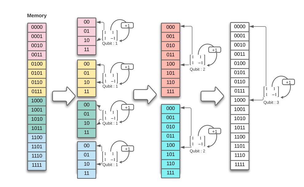
5.2. Thread-level parallelism
When simulating diagonal gates, memory traversals expose significant data-level parallelism exploited by multiple CPU threads. For non-diagonal gates, the recursive FFT-like algorithm also exposes parallelism after simulating gates on the most significant qubits — branches of recursion can be processed by different CPU threads (Figure 11). This brings a 3-4 speedup with 8 threads, but for circuits with qubits the most significant one-qubit gates become a bottleneck due to large memory strides. To simulate those gates in larger circuits, we use a direct algorithm that partitions the state vector into regions processed by parallel threads. To reduce CPU cache misses, we use cache blocking and aligned-memory reads/writes described in Section 5.3. The boundary between the more- and the less-significant qubits (used to choose between the FFT-like algorithm and direct gate application) has only a small impact on the overall runtime, so we keep these two groups as equal in size as possible. In C++ code, we invoke parallel threads using OpenMP pragmas, which can be disabled for sequential execution.
5.3. Data-level parallelism
We achieve major performance gains with aligned memory reads and writes that fetch 256 bits of data (four complex numbers). These optimizations forced us to replace C++ STL vector classes with C-style arrays whose memory positioning can be controlled precisely. Fortunately, all large arrays in quantum circuit simulation are sized at large powers of two, and can therefore be perfectly aligned using a small amount of address arithmetic. When simulating diagonal gates, each pass becomes faster with fewer reads and writes (here we use Gray codes only within each 256-bit block). When simulating pairs of one-qubit gates, our memory traversal pattern is enhanced by cache blocking via the recursive FFT-like algorithm in Figure 10. Cache blocking, shown in Figure 11, also improves temporal locality by allowing us to apply all gates that act on qubits lower than when the block is first read for diagonal gates application - i.e., several traversals of the block are made in a short time-span. Recall that pairs of one-qubit gates are applied to four amplitudes at a time, but those four amplitudes are not contiguous in general. Therefore, we load an entire L1 cache line for each, so that four aligned reads provide data for applying two gates to four sets of amplitudes. Moreover, Section 4.5 clusters one-qubit gates that act on the same qubit(s), and we can now apply those gates on the same L1 cache line loaded into an AVX-2 register to reduce unnecessary memory transfers. Compared to prior work, we do not multiply out clusters of gates as matrices but instead store them in a factored form.
With entire cache lines loaded to AVX-2 registers, we made a concerted effort to leverage wide arithmetic operations from the AVX-2 instruction set. Relevant CPU instructions accessed through compiler intrinsics are listed in Table 1. To prepare registers for AVX-2 arithmetics, 32-bit values may need to be shuffled using several types of bit permutations. CPU cycles can be reduced by optimizing data shuffles and by reducing the number of arithmetic operations. The latter is facilitated by common sub-expression elimination and matrix factorizations.
Example 5.1.
Our AVX-2 kernel to simulate
the gate (Section 4.4)
is illustrated in Figure 12 and 9.
It operates on four AVX-2 registers, each holding two amplitudes
(data supplied by aligned memory reads).
Multiplications by
are performed in parallel by swapping the real and imaginary parts of two amplitudes and then negating their real parts
via bitwise XOR with the -0.0f constant. The instructions _mm256_permute_ps and _mm256_xor_ps
execute in a single cycle on Intel CPUs, whereas multiplication takes 3-5 cycles depending on the CPU.
Our approach saves at least twelve CPU cycles for a pair of gates.
The add and subtract AVX-2 instructions in Figure 12 complete in 24 cycles. Simulating unpaired
single gates requires multiplying by which we reduce to additions, subtractions, permutations and XOR operations.
Customizing such permutations, arithmetic and other instructions to each gate type is a laborious process with careful testing. To reduce CPU cycles, we investigated assembly code generated for compiler intrinsics, and these efforts were rewarded by performance benefits. Here we emphasize the significance of aligned memory reads/writes, which enable AVX-2 arithmetics and also improve bandwidth, keeping more CPU threads supplied with data.
6. Simulation Comparisons
This work targets circuits that run on NISQ computers (Preskill) and are therefore limited in the number of qubits. Among such circuits, many well-known examples are fairly easy to simulate by specialized methods (Viamontes). Therefore, we focus on recent quantum-supremacy circuits from Google (new_benchmarks) that were designed to ensure difficulty of simulation while using gates that support error correction (google_2018). The average-case difficulty of their simulation is proven analytically (bouland_quantum_2018), and the benchmarks have been revised (rr2020, arxiv:1807.10749) to remove unintended simulation shortcuts. Table 3 shows characteristics of the benchmarks, including their large T-gate counts, which defeat stabilizer-based simulation techniques.
Our methods are not limited to Google benchmarks, and our Schrödinger simulator does not exploit some of their well-known features that simplify simulation, such as their planar-grid qubit layout with nearest-neighbor qubit couplings. Therefore, one can expect comparable performance for, e.g., VQE circuits from quantum chemistry (QS_opportunities; quantumChemistry_2020). In addition to pure Schrödinger simulation, our techniques can be used to accelerate layered simulation algorithms (rr2020; teleport2020; IBM2019storage) that handle a greater variety of circuits. For example, divide-and-conquer algorithms leverage Schrödinger simulation of -qubit blocks to simulate -qubit circuits (rr2020). Tables 3 and 4 show results for pure Schrödinger and Schrödinger-Feynman simulation (rr2020) with our optimizations included.
| Gate simulation | RR with opt | RR w/o opt |
|---|---|---|
| passes | % runtime | % runtime |
| Initial H (32) | 7.05 | 0.49 |
| Unmatched final H (12) | 5.46 | 2.23 |
| CZ & T (300), Low | 19.1 | 75.6 |
| X & Y (94) & H (14) | ||
| Single X (5) & Y (1) | 8.46 | 1.54 |
| High X & Y (96) & H (6) | 57.3 | 19.7 |
| Rescaling passes (2) | 2.58 | 0.49 |
| Total (560) | 72s | 2050s |
| Circuit | Gates | Microsoft QDK | QISkit-Aer QASM | Rollright | Ratios QDK/RR | Ratios QISkit/RR | ||||||||
| depth | all | 2-q | T | time | mem | time | mem | mode | time | mem | time | mem | time | mem |
| 1+26+1 | s | MiB | s | MiB | s | MiB | ||||||||
| MacBook Pro 2017 — MacOS High Sierra: 16 GiB, Intel Core i7-7700HQ (2.80GHz) 4 cores 8 threads | ||||||||||||||
16q |
274 | 78 | 68 | 2.34 | — | — | S | — | — | — | — | — | ||
24q |
417 | 123 | 99 | 16.64 | 463 | 3.76 | 128.45 | S | 0.88 | 128 | 18.91 | 3.63 | 4.27 | 1.00 |
25q |
435 | 130 | 105 | 28.72 | 972 | 8.02 | 256.32 | S | 1.45 | 256 | 19.81 | 3.80 | 5.53 | 1.00 |
30q |
524 | 161 | 119 | — | OOM | 346.13 | 8023.39 | S | 58.8 | 8192 | — | — | 5.88 | 1.00 |
| Server — Ubuntu Linux: 144 GiB, Intel Xeon Platinum 8124M (3.00GHz) 18 cores, 72 threads | ||||||||||||||
30q |
524 | 161 | 119 | 1213.16 | 23959 | 18.13 | 8023.39 | S | 17.6 | 8192 | 52.29 | 2.92 | 1.03 | 1.00 |
30q |
524 | 161 | 119 | 1213.16 | 23959 | 18.13 | 8023.39 | S-F | 4.23 | 27 | 4030.43 | 887.38 | 4.28 | 297.16 |
32q |
560 | 168 | 168 | — | OOM | 75.68 | 32022.62 | S | 72.0 | 32000 | — | — | 1.05 | 1.00 |
32q |
560 | 168 | 168 | — | OOM | 75.68 | 32022.62 | S-F | 0.492 | 48 | — | — | 153.82 | 667.13 |
36q |
633 | 195 | 144 | — | OOM | — | OOM | S-F | 90.03 | 192 | — | — | — | — |
6.1. Validation and runtime profile data
We implemented our algorithms in C++17 with OpenMP in a package called Rollright, compiled with Clang v11.0.3. As seen in Section 5.3 we use AVX-2 instructions available on commodity and server CPUs. To validate simulation results up to 25 qubits, we saved all amplitudes of final states and checked them using several industry and academic simulators. For circuits with 30-36 qubits, we checked a few amplitudes with the authors of Google benchmarks.
Our experiments started on a MacBook Pro 2017 laptop with 16 GiB RAM, where our baseline Schrödinger simulation completes a 30-qubit circuit with depth in 72 s using a little over 8 GiB of RAM (1+ and +1 denote initial and final layers of Hadamard gates as in Figure 8). Runtimes are consistent among different circuits of similar size. On the laptop, we use a single CPU process with eight threads. For simulations on a midrange server with ample memory (Tables 3 and 4) we use multiple CPU processes (with eight threads each) to leverage available hardware threads.
Based on profiling data, I/O and circuit pre-processing take negligible time. The bottlenecks are in simulating clusters of diagonal and non-diagonal gates. We further distinguish non-diagonal gates acting on the more and the less significant qubits. To illustrate, for a -qubit Google circuit of depth , simulating and gates on the more significant qubits took of runtime. But gates and remaining , , gates took runtime.
Table 2 breaks down the runtimes of a fully optimized (with opt) and an unoptimized (w/o opt) versions of Rollright on a 32-qubit Google circuit. Initial H gates are a separate category because they are simulated by initializing all amplitudes to the same value (1) and setting the carried over power of accordingly. Being diagonal, CZ and T gates are simulated in one pass by the optimized version. Low-qubit X, Y and H gates are simulated during the same pass, so as to reduce memory transfers. On each L1 cache line loaded into an AVX-2 register by aligned memory read (and later stored by aligmed memory write), we simulate all applicable gates.
We see that for the unoptimized version, runtime is dominated by this joint pass (75.6%) and the next category includes high-qubit X, Y and H gates (19.7%). The optimized version is 28.5 times faster and significantly reduces the time taken by diagonal and low-qubit gates (19.1%), but runtime is dominated by high-qubit X, Y and H gates (57.3%). This is not surprising since our simulation of diagonal gates uses asymptotically fewer memory passes and exposes abundant thread-parallelism, whereas high-qubit non-diagonal gates entail multiple memory passes with large strides and limited thread parallelism. Note that we have similar numbers of low- and high-qubit X,Y gates, but high-qubit gates take much longer to simulate. Among the remaining gate categories are unpaired (single) X and Y gates, as well as a handful of unmatched trailing H gates, which take single-percent fractions of total runtime.
The apparent dominance of memory accesses over computation during optimized simulation suggests limits to further optimization. Memory throughput is also likely to become an issue when porting our algorithms to GPUs or FPGAs.
6.2. Ablation experiments
In order to demonstrate the impact of individual optimizations on Rollright’s performance, we turn them off one by one and plot the resulting runtimes in Figure 14. In these experiments, the full configuration of Rollright uses eight threads. Separate lines are shown for runtime without optimizations for diagonal gates, without one-qubit gates clustered by L1 cache lines and the FFT-like algorithm, without AVX-2 instructions, and without aligned read-write operations. Note that without aligned read-writes, clustering by L1 cache lines makes no sense, and data for AVX-2 instructions are not readily available in AVX-2 registers. We also show runtime with all optimizations turned off — a baselime Schrödinger simulation that applies gates one by one.
Figure 14 suggests that aligned read-write and AVX instructions impact runtime by more than other individual optimizations, especially for circuits with over 30 qubits (in addition to the more efficient memory transfer, aligned read-write ops appear to improve CPU cache utilization). However, the cumulative impact of all optimizations far exceeds the impact of any one optimization.
6.3. Comparisons to Microsoft, IBM and Google
We compared our simulator to the Microsoft Quantum Development Kit (QDK) v0.2.1806.3001 and IBM QISKit Aer v0.6.1. Among simulations in IBM QISkit, we found QASM to be the fastest on quantum-supremacy circuits (GoogleSuprem; new_benchmarks). Table 3 reports comparisons on circuits of depth with up to 36 qubits. To exclude code segments from memory comparisons, we first measured max resident memory for each simulator on the 16-qubit benchmark and then used those measurements as baselines. Memory differences among Schrödinger simulations, when present, are mostly due to our use of single-precision floats. Rollright’s advantage in runtime is greater and grows with the number of qubits.
For 30-qubit circuits, the Microsoft simulator required 16 GiB memory (Rollright used a little over 8 GiB), so we also used a multicore Linux server with sufficient memory and observed that the Microsoft and IBM simulators used all available threads. The optimizations proposed in this work apply to both Schrödinger and Schrödinger-Feynman simulation, therefore we evaluated Rollright in both modes. Clearly, the Schrödinger-Feynman simulation offers a much greater advantage in both runtime and memory on circuits of depth 1+26+1. The 32-qubit circuit uses the oblong qubit array, and the Schrödinger-Feynman mode of our simulator is able to exploit this shape. Therefore, we also show results for Schrödinger-Feynman simulation on an even-sided qubit array. Our comparisons to software from IBM and Microsoft have been presented in person at these companies and helped IBM find a bug, bringing QISKit Aer memory usage down to match ours.
| q | q | q | q | ||||
| S | S-F | S | S-F | S | S-F | S-F | |
| Qsim | 1.1 | 1.64 | 24.25 | 0.47 | 152 | 0.75 | 194.12 |
| RR | 0.77 | 1.26 | 17.60 | 4.23 | 72.40 | 0.49 | 94.48 |
| ratio | 1.43 | 1.30 | 1.38 | 0.11 | 2.09 | 1.53 | 2.05 |
We also compared our simulator to the Qsim simulator under development at Google (https://github.com/quantumlib/qsim). According to the authors, Qsim clusters one-qubit gates to nearby two-qubit gates and uses AVX-2 instructions to simulate resulting generic two-qubit gates one by one. Qsim lacks our optimizations for diagonal and one-qubit gates, as well as the FFT-like algorithm that optimizes memory access. Following our prior collaboration with Google (rr2020), Qsim supports the same simulation modes as Rollright — Schrödinger and Schrödinger-Feynman, — which facilitates more detailed apples-to-apples comparisons. Runtimes in Table 4 (shared with Qsim authors) were collected on the same server as for the lower half of Table 3. While Google Qsim outperforms IBM QISkit and Microsoft QDK on Google benchmarks, Rollright remains ahead, confirming the impact of our proposed methods.
6.4. Scalability studies and use models
Table 15 shows simulator performance for varying numbers of CPU threads. Different simulators exhibit similar scaling, with Rollright remaining ahead in all cases. The results in Table 3 show massive advantage of Schrödinger-Feynman simulation, but pure Scrödinger simulation remains attractive for deep quantum circuits, e.g., in quantum chemistry applications (QS_opportunities; quantumChemistry_2020) and/or when supercomputing resources are available (de_raedt_massively_2007; wecker2014liquid; de_raedt_massively_2018; PB; qHIPSTER; IBM2017breaking; Taihu; IBM2019storage). and runtime as . Simulating 40-qubit circuits this way would require servers with 8 TiB (now available from Microsoft Azure and Amazon AWS). In the Schrödinger-Feynman mode, memory usage can be kept low (see details in (rr2020)) by serializing the computation, but if massive parallel resources are available, using greater peak memory can decrease the latency of simulation. In the meantime, runtime grows as for a large . Figure 13 uses larger supremacy benchmarks from Google to illustrate these differences between Schrödinger and Schrödinger-Feynman simulation by plotting memory usage and runtime for varied qubit counts and circuit depth. The linear runtime of Schrödinger simulation vs. circuit depth (regardless of gate typess) improves upon the semi-exponential scaling of Schrödinger-Feynman simulation.
Distributed Schrödinger-Feynman simulations with Rollright in Google Cloud (rr2020) show that our methods are relevant to boundeded-depth 56- and 64-qubit circuits. Our methods also fit in unbounded-depth Schrödinger simulations on supercomputers (Taihu). Results in (teleport2020) cast the simulation of shallow wide circuits to that of deep narrow circuits, where pure Schrödinger simulation does well.
7. Conclusions
Near-term intermediate-scale quantum (NISQ) computers (Preskill) are operating with 64 qubits in 2020. Quantum circuits running on such computers support many science experiments (QS_opportunities) and motivate circuit optimization tasks, which often require simulation on conventional computers. Recent advances in quantum chemistry offer synthesis methods for NISQ circuits that model molecular configurations and compute their energy levels. Here quantum-circuit simulation is needed to develop and validate advanced quantum technologies, such as quantum-on-quantum simulators (QS_opportunities).
Among the many simulation algorithms, this work focuses on Schrödinger simulation that can be used independently or in layered simulation algorithms (rr2020; teleport2020; IBM2019storage) that handle a greater variety of circuits. Our algorithmic optimizations collectively provide hefty speed-ups over quantum simulators from Microsoft and IBM on hard circuits from Google. These speedups are not limited by a constant factor, but grow with the number of qubits. Our high-level and some low-level optimizations — gate clustering by type, aligned memory reads/writes, gate clustering by cache line, fast simulation of diagonal gates, the recursive FFT-like algorithm, — are generic. Low-level optimizations are tuned to gates that support quantum errror correction, are available on Google chips and are used in Google benchmarks (GoogleSuprem; new_benchmarks). Additional gates can be supported natively or by expressing them in terms of native gates.
For evaluation, we use medium-size circuits which most industry simulators can handle today, but our contributions help with many more qubits as shown in (rr2020; teleport2020) and directly benefit supercomputing simulations (Taihu). Pure Schrödinger simulation is well-suited for deep circuits for VQE algorithms in quantum chemistry (QS_opportunities; quantumChemistry_2020).
Acknowledgements.
We thank Dmitri Maslov, Sergio Boixo and Sergei Isakov for insightful comments.References
- (1) Nielsen, M. A. & Chuang, I. L. Quantum Computation and Quantum Information (10th Anniversary edition). Cambridge . Press (2016), 978-1-10-700217-3, 1-676.
- (2) Preskill, J. Quantum computing and the entanglement frontier (2012). 25th Solvay Conf.
- (3) Boixo, S. et al. Characterizing quantum supremacy in near-term devices. Nat. Phys. 14, 595 (2018). arXiv:1608.00263.
- (4) Arute, F. & Arya, K. & Babbush, R. & et al Quantum supremacy using a programmable superconducting processor. Nature 574, 505–510 (2019) Nature 575, 505-510 (2019). arXiv:1910.11333.
- (5) Aaronson, S. & Chen, L. Complexity-theoretic foundations of quantum supremacy experiments. arXiv:1612.05903 (2016).
- (6) Bouland, A., Fefferman, B., Nirkhe, C. & Vazirani, U. On the complexity and verification of quantum random circuit sampling. Nature Phys 15, 159–163 (2019).
- (7) Aaronson, S. & Gottesman, D. Improved Simulation of Stabilizer Circuits. Phys. Rev. Lett. 70, 052328 (2004).
- (8) Viamontes, G. F., Markov, I. L. & Hayes, J. P. Quantum circuit simulation. Springer Science & Business Media, 2009.
- (9) Markov, I.L. & Shi, Y. Simulating Quantum Computation by Contracting Tensor Networks.. SIAM J. Comput., 38(3), 963–981 (2008).
- (10) Altman, E. et al. Quantum Simulators: Architectures and Opportunities. arXiv:1912.06938 (2019).
- (11) De Raedt, H. et al. Massively parallel quantum computer simulator. Computer Physics Communications 176, 121–136 (2007).
- (12) De Raedt, H. et al. Massively parallel quantum computer simulator, eleven years later. arXiv:1805.04708 (2018).
- (13) Wecker, D. & Svore, K., M. LIQUi|>: A Software Design Architecture and Domain-Specific Language for Quantum Computing. arXiv:1402.4467 (2014).
- (14) Häner, T. & Steiger, D. S. 0.5 Petabyte Simulation of a 45-Qubit Quantum Circuit. arXiv:1704.01127 (2017).
- (15) Smelyanskiy, M., Sawaya, N. P. D., qHiPSTER: The Quantum High Performance Software Testing Environment arXiv:1601.07195 2017
- (16) Pednault, E. et al. Breaking the 49-qubit barrier in the simulation of quantum circuits. arXiv:1710.05867 (2017).
- (17) Villalonga, B. et al. Establishing the Quantum Supremacy Frontier with a 281 Pflop/s Simulation. Quantum Science and Technology 5, 034003 (2020).
- (18) Pednault, E et al. Leveraging Secondary Storage to Simulate Deep 54-qubit Sycamore Circuits. arXiv:1910.09534 (2019).
- (19) Li, R., Wu, B., Ying, M., Sun, X. & Yang, G. Quantum supremacy circuit simulation on Sunway TaihuLight. arXiv:804.04797 (2018).
- (20) Chen, M.-C. et al. Quantum-Teleportation-Inspired Algorithm for Sampling Large Random Quantum Circuits. arXiv:1901.05003. Phys. Rev. Lett. 128, 080502 (2020).
- (21) Markov, I.L. & Fatima, A. & Isakov, S. & Boixo, S. Massively parallel simulation of hard quantum circuits. DAC 2020 arXiv:1807.10749 (2018).
- (22) Ekert, A., Hayden, P. & Inamori, H. Basic concepts in quantum computation. arXiv:quant-ph/00110137 (2000).
- (23) Shi, Y. Both Toffoli and Controlled-NOT need little help to do universal quantum computation. arXiv:quant-ph/0205115 (2002).
- (24) Boixo, S. & Neill, C. The question of quantum supremacy. Google AI Blog (2018). Benchmarks available on GitHub at https://github.com/sboixo/GRCS.
- (25) A Preview of Bristlecone, Google’s New Quantum Processor, Google AI Blog (2018).
- (26) Ogita, T. & Rump, S. M. & Oishi, S. Accurate sum and dot product. SIAM J. on Scientific Computing 26(6), 1955-1988 (2005).
- (27) Bullock, S. S. & Markov, I. L. Asymptotically Optimal Circuits for Arbitrary N-Qubit Diagonal Comutations. Quantum Info. Comput. 4, 27-47 (2004).
- (28) Ruiz-Perez, L. & Garcia-Escartin, J. C. Quantum arithmetic with the quantum Fourier transform. Quantum Information Processing 16, 152 (2017).
- (29) McArdle, Sam. & Endo, Suguru & Aspuru-Guzik, Alán & Benjamin, Simon, C. & Yuan, Xiao Quantum computational chemistry. Rev. Mod. Phys. 92, 015003 (2020)