03Thanks: *: equal contribution. Order is determined through dice rolling. Correspondence to: Xian Wu (xwu9@nd.edu)CCS: Information systems Data miningCCS: Applied computing Electronic commerce

Jiatu Shi^1∗, Huaxiu Yao^2∗, Xian Wu³, Tong Li¹, Zedong Lin¹, Tengfei Wang¹, Binqiang Zhao¹ Affiliation: ¹Alibaba Group, ²Pennsylvania State University, ³University of Notre Dame email: jiatu.sjt, litong.lt, zedong.lzd, wenlin.wtf, binqiang.zhao@alibaba-inc.com email: huaxiuyao@psu.edu, xwu9@nd.edu

2021; © acmcopyright

Abstract.

E-commerce business is revolutionizing our shopping experiences by providing convenient and straightforward services. One of the most fundamental problems is how to balance the demand and supply in market segments to build an efficient platform. While conventional machine learning models have achieved great success on data-sufficient segments, it may fail in a large-portion of segments in E-commerce platforms, where there are not sufficient records to learn well-trained models. In this paper, we tackle this problem in the context of market segment demand prediction. The goal is to facilitate the learning process in the target segments by leveraging the learned knowledge from data-sufficient source segments. Specifically, we propose a novel algorithm, RMLDP, to incorporate a multi-pattern fusion network (MPFN) with a meta-learning paradigm. The multi-pattern fusion network considers both local and seasonal temporal patterns for segment demand prediction. In the meta-learning paradigm, transferable knowledge is regarded as the model parameter initialization of MPFN, which are learned from diverse source segments. Furthermore, we capture the segment relations by combining data-driven segment representation and segment knowledge graph representation and tailor the segment-specific relations to customize transferable model parameter initialization. Thus, even with limited data, the target segment can quickly find the most relevant transferred knowledge and adapt to the optimal parameters. We conduct extensive experiments on two large-scale industrial datasets. The results justify that our RMLDP outperforms a set of state-of-the-art baselines. Besides, RMLDP has been deployed in Taobao, a real-world E-commerce platform. The online A/B testing results further demonstrate the practicality of RMLDP.

Keywords:

Market Segment Demand Prediction; periodicity; Segment Relation Extraction

1. Introduction

Large-scale E-commerce platforms (e.g., Amazon, Taobao) are revolutionizing people’s shopping experience by providing numerous merchandise options at one’s fingertips. To build an efficient E-commerce platform, one of the most fundamental problems is how to balance the demand and supply in the market, which requires an accurate demand prediction model for every market segment (e.g., wallet, belt). An accurate demand prediction model benefits the platform from three aspects: 1) pre-allocate resources to meet the market demand; 2) reduce the backlog of commodities; 3) optimize the allocation strategies of traffic source. In addition, due to the lags between upstream and downstream of the supply chain, real-time segment demand prediction (e.g., predict the next day’s demand) may be impractical. Instead, given the historical demand records, we study the demand prediction problem as predicting the demand value of a future target period (e.g., one month) several weeks in advance (as illustrated in Figure 1).

Figure 1. Illustration of Segment Demand Prediction.

To predict market segment demand, traditional ensemble models (e.g., XGBoost (Chen and Guestrin 2016)) and advanced deep learning methods (e.g., LSTM (Hochreiter and Schmidhuber 1997), GRU (Chung et al. 2014)) are capable of capturing time-varying sequential patterns (e.g., seasonal trend) and making accurate predictions. The superiority of these methods relies on large-scale labeled training data. Unfortunately, as illustrated in Figure 2, a large portion of market segments is located in a long-tail position with limited records, which leads to poor prediction performance and, in turn, affects the efficiency of the platform. The reasons are two-fold: 1) Usually, market segments with more records are more likely to be exhibited on the platform. For data-insufficient market segments, the lack of exposure opportunities brings difficulties in collecting new records and negatively affects the model performance on these segments. The process finally forms a vicious circle, resulting in the platform’s homogenization; 2) The data-insufficient market segments have data quality issues. Due to the limited resources (e.g., the number of exhibitions), for data-insufficient market segments, purely rely on platform managers’ support is impractical and may jeopardize the performance of the mainstream segments. Therefore, how to improve the prediction performance for market segments with limited data remains a non-trivial but necessary problem.

Figure 2. Histogram of segment records’ frequencies in Juhuasuan. Both frequency and number of records are normalized due to privacy policy. A large number of segments only have limited records.

To tackle this “small data" problem, recently, knowledge transfer (e.g., transfer learning, meta-learning) (Pan and Yang 2009; Finn et al. 2017) has achieved great success in a series of applications, such as computer vision (Tzeng et al. 2017), natural language processing (Li et al. 2019). To improve target tasks’ learning process with limited labeled data, knowledge transfer leverages the prior knowledge learned from relevant source tasks. In the segment demand prediction, only applying conventional knowledge transfer algorithms to improve the performance of data-insufficient segments faces the following two major challenges:

•

C1: How to boost the stability and generalization ability of knowledge transfer? Usually, the performance of knowledge transfer relies on the similarity of distributions between source and target tasks. Significant data distribution difference between tasks may lead to unstable transfer or even worse prediction performance. Therefore, a sufficiently generalized knowledge transfer framework is required, covering comprehensive and diverse temporal patterns of market segments.
•

C2: How to incorporate the complex relations among market segments? It is non-trivial to capture the complex segment relations using traditional knowledge transfer methods (e.g., fine-tuning), where the transferable knowledge is globally shared across source segments. However, in E-commerce platforms, the differences between segments can not be overlooked, and thus the globally shared transferable knowledge may not be robust enough to all scenarios. For example, the demands of down jackets are probably similar to coats’ demands, while dissimilar to t-shirts. Thus, segment relations are necessary to be incorporated in knowledge transfer framework.

Hence, to address the above challenges, in this paper, we propose a novel framework RMLDP for data-insufficient market segment demand prediction. The goal for RMLDP is to build a customized meta-learning paradigm upon a market demand prediction model. Specifically, we first construct a multi-pattern fusion network (MPFN) for market segment demand prediction, which jointly captures both local and seasonal temporal patterns by two Gated recurrent units (GRUs). Regrading the MPFN as the base model, the first challenge is solved by learning and transferring the model parameter initialization of the MPFN under the meta-learning paradigm. Here, various source segments sampled from diverse categories (e.g., food, clothing) are used for initialization learning. Finally, we introduce a data-driven segment representation and a segment knowledge graph representation to capture the complex segment relations. For each segment, the relational information are further used to modulate the model parameter initialization.

In summary, our major contributions are three-fold:

•

To the best of our knowledge, we are the first to study the problem of market segment demand prediction with limited data by transferring the knowledge from mainstream segments.
•

We develop a novel framework, RMLDP, to solve the market segment demand prediction task. RMLDP incorporates a multi-pattern fusion network with the meta-learning paradigm. The segment relations are further distilled to customize the model parameter initialization in meta-learning paradigm. Furthermore, we deploy the proposed method into the online platform.
•

We collect the market demand records from two large-scale E-commerce platforms: Juhuasuan and Tiantiantemai. Comparing with baseline methods, the superior performance of RMLDP demonstrates the effectiveness of our framework under both offline and online scenarios.

2. Related Work

This section briefly discusses two categories of related work: time series prediction and knowledge transfer.

Time Series Prediction. Traditional approaches (e.g., ARIMA (Pan et al. 2012), Kalman filtering (Lippi et al. 2013)) have been widely used in time series applications. These methods fail to capture complex non-linear temporal correlations due to the limited expressive capability. With stronger expressive power, deep learning methods, especially recurrent neural network-based approaches (e.g., GRU (Chung et al. 2014) and LSTM (Hochreiter and Schmidhuber 1997)), have achieved great success in time series modeling (Qin et al. 2017; Laptev et al. 2017; Lv et al. 2018; Lai et al. 2018; Salinas et al. 2019; Wang et al. 2019; Rangapuram et al. 2018). To further improve the prediction performance, recently, more information have been incorporated in the basic recurrent neural network structures by applying attention mechanism (Qin et al. 2017; Ma et al. 2017) or multi-resolution modeling (Wu et al. 2018; Huang et al. 2019). However, all these methods rely on large-scale training data. In contrast, our work aims to improve the prediction of data-insufficient target segments by knowledge transfer. Besides, those methods focus on the prediction for the next step/a few steps. In this work, we focus on the early forecast for a future time interval under the real-world E-commerce scenario.

Knowledge Transfer. To benefit the learning process on task with limited data, transferring knowledge from its related tasks has achieved great success in recent years (Pan and Yang 2009). Conventional transfer learning methods learn transferable latent factors between one source domain and one target domain. The latent factors are captured by a series of techniques, such as matrix factorization (Long et al. 2013), manifold learning (Gong et al. 2012) and deep learning (Tzeng et al. 2017; Long et al. 2015). Recently, meta-learning (a.k.a., learning to learn) provides a more stable and flexible way for knowledge transfer. The goal for meta-learning is to generalize the knowledge from various tasks and then adapt them to unseen tasks. In meta-learning, the transferable knowledge are regarded as model parameter initializations (Finn et al. 2017; Finn et al. 2018; Lee and Choi 2018; Yao et al. 2019c; Finn and Levine 2018), metric mapping function (Snell et al. 2017; Vinyals et al. 2016; Oreshkin et al. 2018), or meta-optimizer (Ravi and Larochelle 2016; Andrychowicz et al. 2016), etc. In the time series related problems, Oreshkin et al. 2020 briefly discusses the relation between the neural time series prediction and meta-learning meta-learning (Oreshkin et al. 2020). Yao et al. 2019a incorporates the gradient-based meta-learning with a region functionality based memory (Yao et al. 2019a) for spatiotemporal prediction. However, this method relies on the spatial semantic correlations between tasks, which limits its applicability in our problem. To the best of our knowledge, we are the first to study market segment demand prediction with limited records by borrowing relation-aware knowledge from other segments.

3. Preliminaries

In this section, we define some concepts and notations and then formally define our problem. Assuming the whole market is split into $I$ market segments $\{s_{1},\ldots,s_{I}\}$ , each market segment $s_{i}$ represents one category of products (e.g., sweaters, orange juice).

Definition 1 (Market Demand Value) For each segment $s_{i}$ at time step $t_{i}$ , the market demand value $x_{i,t_{i}}$ is defined as the number of purchasing requests in a fixed time window $[t_{i},t_{i}+t^{{}^{\prime}}]$ . In this paper, the length fixed time interval $t^{{}^{\prime}}$ is defined as one day (i.e., $t^{{}^{\prime}}=1$ ).

Definition 2 (Target Demand Value) As illustrated in Figure 1, we aim to predict the market demand for a future target time interval $T_{f}$ several weeks in advance. Supposing the current time stamp is $t_{c}$ and the time lag between the current time and the further target time is $T_{g}$ , we define the target demand value $y_{i,t_{c}}$ as the total market demand value of $s_{i}$ between time interval $[t_{c}+T_{g},t_{c}+T_{g}+T_{f}]$ (i.e., $y_{i,t_{c}}=\sum_{j=T_{g}}^{T_{g}+T_{f}}x_{i,t_{c}+j}$ ).

Problem: Market Segment Demand Prediction with Limited Records Assuming that we have a set of diverse source segments $\{s_{1},\ldots,s_{I}\}$ and a target segment $s_{t}$ with limited records, we aim to predict the target demand value $y_{t,t_{c}}$ in the testing dataset of the target segment. Additionally, for each segment $s_{i}$ at time stamp $t_{c}$ , we further introduce several statistical features $\mathbf{e}_{i,t_{c}}$ (e.g., # of items, sellers, brands) and customers’ action features (e.g., click, collect, add to cart and take order).

We denote the concatenation of market demand value $x_{i,t_{c}}\in\mathbb{R}^{1}$ and external features $\mathbf{e}_{i,t_{c}}\in\mathbb{R}^{e-1}$ as $\mathbf{x}_{i,t_{c}}=x_{i,t_{c}}\oplus\mathbf{e}_{i,t_{c}}\in\mathbb{R}^{e}$ . The market segment demand prediction model (a.k.a., base model) is defined as $f$ with the learnable parameters $\theta$ . Formally, our problem is formulated as:

(1)

\small y_{t,t_{c}}^{*}=\arg\max_{y_{t,t_{c}}}p(y_{t,t_{c}}|\theta_{0t}^{*},\{\mathbf{x}_{t,1},\ldots,\mathbf{x}_{t,t_{c}}\})

where $\theta_{0t}^{*}$ denotes the segment-specific initializations, which are transferred from all source segments using the target segment information. Detailed discussions about customized model initializations are in Section 4.2 and 4.3. We name the process of learning transferable knowledge from source segments as meta-training and the adaption in target segments as meta-testing.

4. Methodology

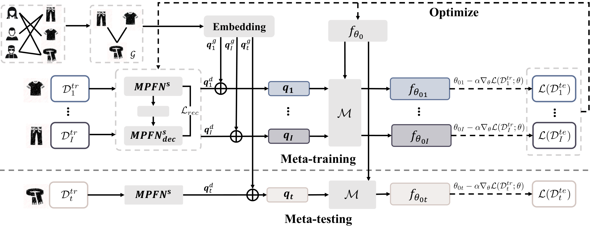
Refer to caption — Figure 3. The Framework of RMLDP. In the meta-training process, the initialization $\theta_{0}$ are customized by using the data-driven segment representation (learned by $\mathrm{MPFN}^{s}$ ) and the representation of segment knowledge graph $\mathcal{G}$ (constructed by users’ purchasing records). The performance on the testing sets of all source segments are further used to update all transferable knowledge (grey blocks). In the meta-testing process, the transferred knowledge is adapted to the target segment $s_{t}$ .

In this section, we introduce our proposed framework: RMLDP (Relation-aware Meta-Learning for Demand Prediction). The whole framework is shown in Figure 3. The goal for RMLDP is to facilitate the learning process of data-insufficient target segment demand prediction by adapting the transferred knowledge (i.e., all grey blocks in Figure 3) from data-sufficient source segments. In particular, the base model $f$ is first designed as a multi-pattern fusion network (MPFN), where both local and seasonal temporal patterns are considered. Then, RMLDP incorporates the base model $f$ and the meta-learning paradigm, where the model parameter initialization are regarded as transferable knowledge. To further modulate the parameter initialization, we distill knowledge from segment representations, including a data-driven segment representation and a segment knowledge graph representation. We detail three key components in the following subsections: multi-pattern fusion network, knowledge transfer, and adaptation, relation-aware modulation.

4.1. Multi-pattern Fusion Network

In this subsection, we propose a multi-pattern fusion network (MPFN) for market segment demand prediction. The framework is illustrated in Figure 4. The goal for MPFN is to predict the target demand value by capturing the temporal patterns from the historical records. To achieve this goal, we adopt a GRU network to capture non-linear relations among historical records. Concretely, for predicting the target demand value $y_{i,t_{c}}$ of segment $s_{i}$ , the most recent $|\mathcal{T}_{c}|$ demand values (i.e., $\{\mathbf{x}_{i,t_{c}-|\mathcal{T}_{c}|+1},\ldots,\mathbf{x}_{i,t_{c}}\}$ ) are fed into the GRU, which is formulated as:

(2)

\small\mathbf{h}^{r}_{i,t_{c}}=\mathrm{GRU}^{r}(\mathbf{h}^{r}_{i,t_{c}-1};\mathbf{x}_{i,t_{c}}).

The temporal representation $\mathbf{h}^{r}_{i,t_{c}}$ encodes the local temporal patterns from the closest records.

As mentioned in Section 3, different from real-time demand prediction, there exists a time lag $T_{g}$ between current time and the target prediction time. Thus, the temporal patterns captured from closest demand records are probably insufficient to achieve satisfactory performance. Fortunately, seasonal temporal patterns provide us with useful periodic information. For example, the demand trend for winter coat in this December is similar to the trend in the last December. However, as suggested in (Yao et al. 2019b), it is non-trivial to train a single GRU network for handling long-term seasonal patterns due to the risk of gradient vanishing. Instead, another GRU network is introduced to model the seasonal patterns as:

(3)

\small\mathbf{h}^{l}_{i,t_{l}}=\mathrm{GRU}^{l}(\mathbf{h}^{l}_{i,t_{l}-1};\mathbf{x}_{i,t_{l}}),

where $t_{l}=t_{c}+T_{g}-365$ represents the corresponding historical time of the target demand value (i.e., same day in the last year). The sequence $\{\mathbf{x}_{i,t_{l}-|\mathcal{T}_{c}|+1}\ldots\mathbf{x}_{i,t_{l}}\}$ are fed into $\mathrm{GRU}^{l}$ .

By fusing the hidden representations $\mathbf{h}^{l}_{i,t_{l}}$ and $\mathbf{h}^{c}_{i,t_{c}}$ as $\mathbf{\hat{h}}_{i,t_{c}}=\mathbf{h}^{l}_{i,t_{l}}\oplus\mathbf{h}^{c}_{i,t_{c}}$ , both local and seasonal temporal patterns are captured. Then, we use one fully connected layer for prediction as:

(4)

\small\hat{y}_{i,t_{c}}=\mathbf{W}_{f}\mathbf{\hat{h}}_{i,t_{c}}+\mathbf{b}_{f},

where $\mathbf{W}_{f}$ and $\mathbf{b}_{f}$ are learnable parameters. In this paper, mean square error (MSE) is used as loss function as:

(5)

\small\mathcal{L}=\sum_{t_{c}}(y_{i,t_{c}}-\hat{y}_{i,t_{c}})^{2}.

As mentioned in Section 3, the MPFN is regarded as base model $f$ with all learnable parameters are denoted as $\theta$ .

Figure 4. Illustration of MPFN for market segment demand prediction.

\mathrm{GRU}^{l}

and

\mathrm{GRU}^{r}

capture seasonal and local temporal patterns, respectively.

4.2. Knowledge Transfer and Adaptation

After constructing the base model MPFN, we discuss the meta-learning paradigm, which transfers knowledge from source segments to the target segment with limited data. To increase knowledge transfer stability, the transferable knowledge is expected to be general enough and contain comprehensive relations between market segments and their historical temporal patterns.

Motivated by the model-agnostic meta-learning (MAML) (Finn et al. 2017), these transferable knowledge are encrypted in the model parameter initialization $\theta_{0}$ of base model $f$ . Thus, the aim of knowledge transfer is to learn an optimal model parameter initialization from multiple source segments $\{s_{1},\ldots,s_{I}\}$ . For segment $s_{i}$ , the model parameters $\theta$ of market demand prediction are updated starting from $\theta_{0}$ as follows:

(6)

\small\theta_{i}=\theta_{0}-\alpha\nabla_{\theta}\mathcal{L}(\mathcal{D}_{i}^{tr};\theta),

where the empirical risk $\mathcal{L}$ is defined as mean square error in Eqn. (5). $\mathcal{D}_{i}^{tr}=\{\mathbf{X}^{tr}_{i,t_{c}},y^{tr}_{i,t_{c}}\}_{t_{c}=1}^{N^{tr}}$ is the training set sampled from segment $s_{i}$ , where $N^{tr}$ denotes the number of training samples and $\mathbf{X}^{tr}_{i,t_{c}}=\{\mathbf{x}^{tr}_{i,t_{l}-|\mathcal{T}_{c}|+1},\ldots,\mathbf{x}^{tr}_{i,t_{l}},\mathbf{x}^{tr}_{i,t_{c}-|\mathcal{T}_{c}|+1},\ldots,\mathbf{x}^{tr}_{i,t_{c}}\}$ represents the used demand sequence in MPFN.

After getting the segment-specific parameter $\theta_{i}$ , we sample the testing dataset $\mathcal{D}_{i}^{te}=\{\mathbf{X}^{te}_{i,t_{c}},y_{i,t_{c}}^{te}\}_{t_{c}=1}^{N^{te}}$ from $s_{i}$ to update the model parameter initialization $\theta_{0}$ by minimizing the empirical risk as:

(7)

\small\theta_{0}\leftarrow\min_{\theta_{0}}\sum_{i=1}^{|I|}\mathcal{L}(\mathcal{D}_{i}^{te};\theta_{i})

where $|I|$ denotes the number of source segments. At the end of meta-training process, we get $\theta^{*}_{0}$ as the learned optimal model parameter initialization.

Given an target segment $s_{t}$ , the segment-specific parameter $\theta_{t}$ is achieve by performing gradient descent starting from the learned initialization $\theta_{0}^{*}$ with the training data $\mathcal{D}_{t}^{tr}$ , i.e.,

(8)

\small\theta_{t}=\theta_{0}^{*}-\alpha\nabla_{\theta}\mathcal{L}(\mathcal{D}_{t}^{tr};\theta).

We finally evaluate the performance by the testing set $\mathcal{D}_{t}^{te}$ of segment $s_{t}$ using adapted parameter $\theta_{t}$ .

4.3. Relation-aware Customization

The above knowledge transfer and adaptation framework regards the transferable knowledge as the globally shared model parameter initialization $\theta_{0}^{*}$ across all source segments. However, the globally shared knowledge may incapable of well-capturing underlying complex segment relations. For example, supposing we need to predict Men’s clothing’s market demand, both local and seasonal temporal trends are similar to clothing from other groups (e.g., women, children), while the temporal trends are probably dissimilar to the electric appliances. Thus, in this section, we tailor the segment-specific relations to modulate the model parameter initialization. Specifically, we consider two types of segment relational representations: data-driven segment representation and segment knowledge graph representation. The data-driven segment representation implicitly encrypts the segment relations. Generated by users’ purchase records, the segment knowledge graph further explicitly models the relations among different segments. We detail these two types of representations in the following subsections.

4.3.1. Data-driven Segment Representation

For data-driven segment representation, we encode the segment-specific information into one representation vector. The relations among segments are implicitly included in the representations since similar segments have similar representations. As suggested in (Vuorio et al. 2019; Yao et al. 2019c), learning the representation of each segment $s_{i}$ is equal to aggregate the training data $\mathcal{D}_{i}^{tr}$ to a representation vector. Here, we introduce one MPFN as aggregator denoted as $\mathrm{MPFN}^{s}$ . The aggregator first encodes each data sample into one vector and then a sample-level mean pooling layer is applied on the top of encoder. Formally, the aggregation process is formulated as:

(9)

\small\mathbf{q}_{i}^{d}=\frac{1}{N^{tr}}\sum_{t_{c}}\mathrm{MPFN}^{s}(\mathbf{X}_{i,t_{c}}^{tr}).

Empirically, only using the loss signal defined in Eqn. (7) to guide the segment representation learning is difficult. To increase the stability of segment representation learning, we introduce the reconstruction loss with a decoder $\mathrm{MPFN}^{s}_{dec}$ , which is defined as:

(10)

\small\mathcal{L}_{rec}=\frac{1}{N^{tr}}\sum_{t_{c}}\|\mathbf{X}_{i,t_{c}}^{tr}-\mathrm{MPFN}^{s}_{dec}(\mathrm{MPFN}^{s}(\mathbf{X}_{i,t_{c}}^{tr}))\|_{F}^{2}

where $\|\cdot\|_{F}$ is defined as Frobenius norm.

4.3.2. Segment Knowledge Graph Representation

In real-world E-commerce platforms, the relations between segments can further be reflected by users’ purchasing records. For each pair of segments, their similarity is proportional to the frequency of co-occurrence in the same order. For example, women usually purchase sweater and skirt together. But it is unlikely to purchase shampoo and refrigerator at the same time. Given users’ purchasing records, we build a segment knowledge graph $\mathcal{G}$ , where each node $n_{i}$ in the knowledge graph represents one segment. For each pair of nodes $n_{u}$ and $n_{v}$ , the link weight $\omega_{uv}$ is calculated by the co-occurrence frequency in the same order. We further set a threshold to filter some low similarity links.

Then, to map each segment into a fixed low dimensional space and maintain their relational structure, we adopt Deepwalk (Perozzi et al. 2014) on the constructed knowledge graph $\mathcal{G}$ . The ad-hoc learned graph embedding vector $\mathbf{u}^{g}_{i}$ is feed into a graph convolutional layer to get the representation of each segment in the knowledge graph, which is denoted as $\mathbf{q}^{g}_{i}=\mathrm{FC}_{\mathbf{W}_{emb}}(\mathbf{u}^{g}_{i})$ . Note that the data-driven segment representation and the segment knowledge graph representation are mutually complementary. In data-driven segment representation, the similarity of segments mainly reflects their temporal patterns. By contrast, the similarity of segments in this knowledge graph are guided by users’ purchasing records.

4.3.3. Relation Fusion and Knowledge Modulation

After generating the data-driven segment representation $\mathbf{q}^{d}_{i}$ and the knowledge graph representation $\mathbf{q}_{i}^{g}$ , we then fuse these two types of representations and get the final segment-specific representation as: $\mathbf{q}_{i}=\mathbf{q}_{i}^{d}\oplus\mathbf{q}_{i}^{g}$ . To customize the globally shared model parameter initialization $\theta_{0}$ , we introduce a modulating function $\mathcal{M}(\cdot)$ , which consists of a mapping layer with an activation function. The modulating function is defined as:

(11)

\small\mathcal{M}(\mathbf{q}_{i})=\sigma(\mathbf{W}_{m}\mathbf{q}_{i}+\mathbf{b}_{m}),

where $\mathbf{W}_{m}$ and $\mathbf{b}_{m}$ are trainable parameters. By using the modulating function, the segment representation is mapped to the same space of the model parameter initialization $\theta_{0}$ . Then, the customization process is formulated as:

(12)

\small\theta_{0i}=\mathcal{M}(\mathbf{q}_{i})\odot\theta_{0},

Here $\theta_{0i}$ represents the task specific parameter initialization. Then, for segment $i$ , we perform the gradient steps starting from the customized initialization $\theta_{0i}$ rather than $\theta_{0}$ .

By combining the empirical risk $\mathcal{L}$ in Eqn. (7) and the reconstruction loss $\mathcal{L}_{rec}$ in Eqn. (10), we revise the objective function in Eqn. (7) and formulate the final objective function as:

(13)

\small\min_{\Theta}\mathcal{L}_{joint}=\min_{\Theta}\sum_{i=1}^{|I|}\mathcal{L}(\mathcal{D}_{i}^{te};\theta_{i})+\lambda\mathcal{L}_{rec},

where the hyperparameter $\lambda$ is used to balance the value of two loss terms. We describe learning process for RMLDP in Algorithm 1.

Input: source segments

\{s_{1},\ldots,s_{I}\}

; learning rate for inner update

\alpha

; meta-learning rate

\beta

; loss weighting factor

\lambda

; length of sequence

|\mathcal{T}_{c}|

Initialize all learnable parameters

\Theta

; 1

while not done do 2

Sample a batch of segments from

\{s_{1},s_{2},\ldots,s_{I}\}

; 3

for each $s_{i}$ do 4

Sample training set

\mathcal{D}_{i}^{tr}

and testing set

\mathcal{D}_{i}^{te}

from

s_{i}

; 5

Calculate the data-driven segment representation

\mathbf{q}_{i}^{d}

by Eqn. (9), reconstruction loss

\mathcal{L}_{rec}

by Eqn. (10); 6

Calculate segment knowledge graph representation

\mathbf{q}_{i}^{g}

and concatenate

\mathbf{q}_{i}^{d}

and

\mathbf{q}_{i}^{g}

\mathbf{q}_{i}

; 7

Use

\mathbf{q}_{i}

to customize the model parameter initialization by Eqn. (12) and get

\theta_{0i}

; 8

Optimize parameters starting from

\theta_{0i}

as:

\theta_{i}=\theta_{0i}-\alpha\nabla_{\theta}\mathcal{L}(\mathcal{D}_{i}^{tr};\theta)

; 9

end for 10

Update

\Theta\leftarrow\Theta-\beta\nabla_{\Theta}\mathcal{L}_{joint}

as Eqn. (13); 11

end while 12

Algorithm 1 Meta-training Framework for RMLDP

5. System Overview

In this section, we introduce the system deployment pipeline of RMLDP in a real-world platform. We independently abstract the strategy center from the E-commerce background management system to implement our algorithm in business scenarios and maintain the low coupling and high cohesion in system design.

In Figure 5, we show the online system. In E-commerce platform, the operators first define the market segments based on a series of field configurations (e.g., the consumer groups served, price ranges of goods, brand collections, etc). The predicted segments are then selected, and the strategy center provides the demand prediction results using the proposed algorithm. Based on the prediction results, each segment’s reasonable market flow resource is determined and sent to the background system. The background system assigns the specific display time and the display channel for each segment. Finally, the segment-specific information are displayed in the consumers’ client App.

With the rapid development of cloud computing technology, behavioral logs (e.g., detailed product information, user’s click, and purchase records on the client) are collected back to cloud storage in real-time. Based on this data, the MapReduce task deployed in the cloud extracts the required features and provides a steady feature stream. With the help of GPU, the model is efficiently trained. The whole system forms a complete closed loop.

6. Experiments

In this section, we conduct comprehensive experiments to evaluate our proposed RMLDP by answering the following research questions: (1) How is the overall prediction performance of RMLDP compared with state-of-the-art baselines? (2) How do various components we proposed (e.g., market segment knowledge graph) impact the model’s performance? (3) How is the online performance of RMLDP based on our proposed method and system?

6.1. Experimental Setups

In the experiment settings, we describe two real-world datasets and the compared baselines. The mean absolute percentage error (MAPE) are used to evaluate the performance.

6.1.1. Dataset Description

To evaluate our proposed method, we collect the data from two large-scale marketing scenarios in Taobao, the largest E-commerce platform in China (tao 2020). We detail the descriptions as follows:

•

Juhuasuan (juh 2020): The first dataset is collected from Juhuasuan, one of the largest platform for group buying in China. There are more than 4000 segments over 800 days. We select three coarse-grained categories (electric appliances, clothing, and daily supplies) with nine fine-grained categories (large electric appliances, small electric appliances, digital electric appliances, women’s clothing, men’s clothing, sports, food, daily chemicals, daily sundry).
•

Tiantiantemai (tia 2020): Another dataset collected from Tiantiantemai, one of the largest platform for low-cost products in China. There are more than 6000 market segments over 189 days. The segments are selected from 3 coarse-grained categories (house hold, clothing, food) with 9 fine-grained categories (kitchenware, bedding, toiletries, womens’ clothing, men’s clothing, children’s clothing, snacks, fresh, drink).

For both Juhuasuan and Tiantiantemai, we sort all segments by the number of purchasing records. We select top 70% segments with more records for meta-training and the rest for meta-validation and meta-testing. For each fine-grained category in Juhuasuan and Tiantiantemai, in this experiment, the averaged performance (MAPE) over all segments with this category are reported.

6.1.2. Hyperparameter Settings

In Table 1, we list all hyperparameters of Juhuasuan and Tiantiantemai.

Table 1. Hyperparameter Settings.

Hyperparameter	Juhuasuan	Tiantiantemai
batch size	128	128
feature dimension	48	48
sequence length $\|\mathcal{T}_{c}\|$	30	30
GRU embedding dimension	128	128
dimension of $\mathbf{q}_{i}^{d}$	32	32
dimension of $\mathbf{q}_{i}^{g}$	16	16
learning rate $\alpha$	$10^{-4}$	$10^{-4}$
meta-learning rate $\beta$	$10^{-3}$	$10^{-3}$
loss factor $\lambda$	0.5	0.5

6.1.3. Baselines

We compare our proposed method with the following four types of baselines: (1) Basic regression methods: Linear Regression, Support vector regression (SVR); (2) Ensemble regression methods: Random Forest, XGBoost (Chen and Guestrin 2016); (3) Neural-network-based methods: GRU, Dipole (Ma et al. 2017), LSTNet (Lai et al. 2018). For GRU and Dipole, we use the MPFN as backbone models and denote these two methods as GRU+MPFN and Dipole+MPFN, respectively. (4) Transfer methods: Fine-tuning, MAML (Finn et al. 2017), Meta-SGD (Li et al. 2017). In Fine-tuning, we use the same strategy as GRU+MPFN to learn the model parameters. Then, we finetune the learned parameters for each target segment. For all baselines, we use the same features as RMLDP. In basic regression, ensemble regression, and neural-network-based methods, the training dataset includes samples from all source segments and the training samples from target segments for a fair comparison.

Table 2. Overall Performance of Juhuasuan.

Model	Electric Appliances			Clothing			Daily Supplies
Model	Large	Small	Digital	Women	Men	Sports	Food	Chemicals	Sundry
Linear Regression	42.19%	43.26%	41.43%	46.32%	47.13%	47.94%	41.02%	42.24%	43.97%
SVR	30.16%	29.26%	30.06%	34.45%	35.56%	36.94%	30.11%	30.31%	33.12%
Random Forest	$26.51$ %	$27.41$ %	$26.58$ %	$28.53$ %	$29.36$ %	$30.55$ %	$26.49$ %	$26.84$ %	$27.29$ %
XGBoost (Chen and Guestrin 2016)	$25.38$ %	$26.81$ %	$25.19$ %	$27.49$ %	$28.37$ %	$28.76$ %	$26.93$ %	$26.53$ %	$26.07$ %
GRU+MPFN (Chung et al. 2014)	$25.62$ %	$26.34$ %	$25.46$ %	$27.51$ %	$27.34$ %	$29.06$ %	$27.09$ %	$26.67$ %	$26.33$ %
Dipole+MPFN (Ma et al. 2017)	$25.53$ %	$26.07$ %	$25.37$ %	$27.43$ %	$27.05$ %	$28.86$ %	$27.01$ %	$26.27$ %	$26.20$ %
LSTNet (Lai et al. 2018)	25.98%	26.66%	26.31%	27.48%	27.56%	29.13%	28.93%	26.94%	26.89%
Finetune	24.29%	26.20%	24.13%	27.12%	26.98%	28.23%	26.54%	26.01%	26.01%
MAML (Finn and Levine 2018)	24.21%	26.08%	23.53%	26.77%	26.51%	27.93%	25.79%	25.04%	25.99%
RMLDP^∗	23.96%	25.29%	22.84%	26.21%	25.87%	26.98%	24.25%	24.38%	25.11%

*: comparing with MAML, the results of RMLDP are significant according to Student’s t-test at level 0.01.

Table 3. Overall Performance of Tiantiantemai.

Model	Household			Clothing			Food
Model	Kitchenware	Bedding	Toiletries	Women	Men	Children	Snacks	Fresh	Drink
Linear Regression	56.89%	47.29%	55.68%	47.51%	49.98%	46.45%	49.64%	53.53%	54.11%
SVR	37.16%	36.26%	38.25%	37.81%	38.94%	38.55%	38.29%	38.19%	39.25%
Random Forest	31.21%	30.41%	31.45%	29.40%	31.35%	29.15%	30.81%	30.84%	31.92%
XGBoost (Chen and Guestrin 2016)	31.16%	30.81%	30.86%	29.49%	31.43%	29.46%	30.13%	30.49%	31.07%
GRU+MPFN (Chung et al. 2014)	31.62%	30.34%	30.33%	29.48%	31.91%	29.71%	30.19%	30.67%	31.03%
Dipole+MPFN (Ma et al. 2017)	30.97%	29.89%	30.01%	29.41%	30.69%	30.12%	30.14%	30.33%	30.66%
LSTNet (Lai et al. 2018)	31.49%	30.76%	30.12%	30.09%	30.98%	30.01%	30.84%	31.16%	31.98%
Finetune	30.49%	29.56%	29.54%	29.27%	30.86%	29.49%	30.10%	30.01%	30.52%
MAML (Finn and Levine 2018)	29.55%	29.08%	29.41%	29.06%	30.07%	29.31%	29.97%	29.84%	30.01%
RMLDP^∗	28.54%	28.19%	28.85%	27.93%	28.56%	28.41%	29.02%	29.34%	29.17%

*: comparing with MAML, the results of RMLDP are significant according to Student’s t-test at level 0.01

6.2. Results

6.2.1. Overall Performance

After implementing our proposed model and comparing it with other baselines, we report the results for Juhuasuan and Tiantiantemai in Table 2 and Table 3, respectively. For each fine-grained category, the averaged MAPE over segments in this category are reported. According to these results, we draw the following conclusions:

•

All other types of baselines significantly outperform the basic regression methods (i.e., Linear regression, SVR). The reason is that it is non-trivial to capture complex non-linear temporal patterns through the basic regression methods.
•

All transfer learning methods (i.e., MAML, Finetune and RMLDP) achieves better performance than other non-transfer methods. The results suggest that finetuning the learned knowledge from other segments can capture the task-specific information in the target segment and further benefit the performance.
•

In all cases, our RMLDP outperforms other baselines. In particular, RMLDP achieves better performance than MAML, which indicates the effectiveness of customizing model parameter initialization by leveraging the complex relations across market segments. Combining with the segment relations, the stability and diversity of transferred knowledge increases to the highest degrees.

6.2.2. Ablation Study

We further perform comprehensive ablation studies to demonstrate the effectiveness of proposed components. We describe the ablation models as follows:

•

RMLDP-d: In RMLDP-d, we remove the data-driven segment representation and only use the segment knowledge graph representation to modulate the model parameter initialization.
•

RMLDP-g: In RMLDP-g, the segment knowledge graph is removed, and the data-driven market segment representation is the only signal for customizing model parameter initialization.
•

RMLDP-szn: We only consider the local temporal trend in RMLDP-szn, i.e., the $\mathrm{GRU}^{l}$ is removed in the base learner MPFN.
•

RMLDP-local: Contrary to RMLDP-szn, in RMLDP-local, we remove $\mathrm{GRU}^{r}$ in the base learner MPFN.

The results for Juhuasuan and Tiantiantemai are reported in Table 4 and Table 5, respectively. The performance of RMLDP is also reported for comparison. From these tables, we observe that:

•

RMLDP performs better than both RMLDP-d and RMLDP-g, indicating the effectiveness and complementarity of segment knowledge graph representation and data-driven representation.
•

Comparing with RMLDP-d, RMLDP-g achieves better performance. The potential reason is that the data-driven market segment representations, which are learned from training data of each segment, capture the segment-specific temporal patterns, and provide more effective information.
•

RMLDP significantly outperforms RMLDP-szn and RMLDP-local, indicating that both local and seasonal temporal patterns contribute to the model performance. The seasonal temporal patterns provide the basic estimation for the segment demand, and the local temporal patterns further provide the calibration by using the most recent records.

Table 4. Ablation studies of Juhuasuan.

Model	Electric Appliances			Clothing			Daily Supplies
Model	Large	Small	Digital	Women	Men	Sports	Food	Chemicals	Sundry
RMLDP-d	24.18%	26.03%	23.41%	26.45%	26.47%	27.84%	25.63%	25.01%	25.97%
RMLDP-g	24.09%	25.84%	22.97%	26.28%	26.01%	27.53%	24.81%	24.77%	25.44%
RMLDP-szn	28.01%	27.97%	26.67%	33.29%	34.72%	35.88%	29.31%	29.34%	31.51%
RMLDP-local	30.42%	31.38%	31.23%	34.98%	35.87%	37.32%	33.09%	31.09%	33.49%
RMLDP	23.96%	25.29%	22.84%	26.21%	25.87%	26.98%	24.25%	24.38%	25.11%

Table 5. Ablation studies of Tiantiantemai.

Model	Household			Clothing			Food
Model	Kitchenware	Bedding	Toiletries	Women	Men	Children	Snacks	Fresh	Drink
RMLDP-d	29.35%	29.07%	29.36%	29.01%	29.96%	28.53%	29.89%	29.78%	29.86%
RMLDP-g	28.91%	28.65%	29.04%	28.09%	29.33%	29.08%	29.15%	29.41%	29.31%
RMLDP-szn	33.83%	33.54%	34.99%	37.36%	36.78%	37.98%	37.54%	36.54%	38.27%
RMLDP-local	41.96%	37.29%	42.53%	40.15%	42.39%	40.49%	41.04%	42.93%	41.45%
RMLDP	28.54%	28.19%	28.85%	27.93%	28.79%	28.41%	29.02%	29.34%	29.17%

6.2.3. Effect of Sequence Length

In this section, we analyze the effect of sequence length (i.e., the value of $|\mathcal{T}_{c}|$ ). We change the sequence length from 15 to 40, and the results for each coarse-category of two datasets are shown in Figure 6. We can see that the MAPE decreases at the beginning and then keeps stable/slightly increases. The reason is that too short sequence may not provide enough information for accurate prediction. When the length of sequence increases, the covered information gradually becomes saturated, and the results keep stable.

6.2.4. Analysis of Segment Representation

We further analyze the segment representation $\mathbf{q}_{i}$ discussed Section 4.3.3, where 694 meta-testing segments in Juhuasuan are used. The results are shown in Figure 7. We observe that the segment representations are capable of well-distinguishing different categories of segments and further provide qualitative evidence for the effectiveness of RMLDP.

Figure 7. Visualization of learned segment representation from 694 meta-testing segments.

6.2.5. Online Experiment

To further evaluate the proposed model, we design the online experiments in Taobao mobile App. We conduct a bucket testing (i.e, A/B testing) in Tiantiantemai to test the consumers’ response to our RMLDP and baseline. For each segment, the higher demand prediction value it gets, the more opportunities of display it gains.

Without using prediction model, operators usually leverage the averaged demand value from the same period of the last year and the nearest month to predict the future demand. In offline evaluation, the MAPE for this statistical method is more than 0.8. We regard this statistical method as our baseline, and calculate five core indicators: Page View (PV), Unique Visitor (UV), total number of segments with orders (#Seg), total number of products with orders (#Item), weekly orders (Ord). The results are reported in Table 6. Except for the supply for different market segments, both buckets have the same personalization strategy of recommendation system. Comparing with the statistical method, our model achieves better performance under the similar volumes of PageView and Unique Visitor.

Table 6. The results of different prediction strategies

Bucket	PV	UV	#Seg	#Item	Ord
Stat. Method	1.93M	0.64M	1334	3708	91980
RMLDP	1.92M	0.64M	1458	3809	94780

7. Conclusion

In this paper, we propose a novel relation-aware meta-learning framework, RMLDP, for market segment demand prediction with limited data by transferring knowledge from data-sufficient segments. Our proposed method incorporates the base demand prediction model (i.e., multi-pattern fusion network) into a meta-learning paradigm. The model parameter initialization learned from source segments can be easily adapted to each target segment. Additionally, the segment relations are learned and tailored to customize the transferable model initialization. Extensive experiments on two large-scale E-commerce datasets verify the effectiveness of RMLDP. RMLDP is further deployed in the real-wold platform with the positive bucket testing results.

References

(1)
juh (2020) 2020. Juhuasuan. https://ju.taobao.com/.
tao (2020) 2020. Taobao. https://www.taobao.com/.
tia (2020) 2020. Tiantiantemai. https://tejia.taobao.com/.
Andrychowicz et al. (2016) Marcin Andrychowicz, Misha Denil, Sergio Gomez, Matthew W Hoffman, David Pfau, Tom Schaul, Brendan Shillingford, and Nando De Freitas. 2016. Learning to learn by gradient descent by gradient descent. In NeurIPS. 3981–3989.
Chen and Guestrin (2016) Tianqi Chen and Carlos Guestrin. 2016. Xgboost: A scalable tree boosting system. In Proceedings of the 22nd ACM SIGKDD International Conference on Knowledge Discovery and Data Mining. ACM, 785–794.
Chung et al. (2014) Junyoung Chung, Caglar Gulcehre, KyungHyun Cho, and Yoshua Bengio. 2014. Empirical evaluation of gated recurrent neural networks on sequence modeling. arXiv preprint arXiv:1412.3555 (2014).
Finn et al. (2017) Chelsea Finn, Pieter Abbeel, and Sergey Levine. 2017. Model-Agnostic Meta-Learning for Fast Adaptation of Deep Networks. In ICML. 1126–1135.
Finn and Levine (2018) Chelsea Finn and Sergey Levine. 2018. Meta-learning and universality: Deep representations and gradient descent can approximate any learning algorithm. In ICLR.
Finn et al. (2018) Chelsea Finn, Kelvin Xu, and Sergey Levine. 2018. Probabilistic Model-Agnostic Meta-Learning. In NeurIPS.
Gong et al. (2012) Boqing Gong, Yuan Shi, Fei Sha, and Kristen Grauman. 2012. Geodesic flow kernel for unsupervised domain adaptation. In Computer Vision and Pattern Recognition (CVPR), 2012 IEEE Conference on. IEEE, 2066–2073.
Hochreiter and Schmidhuber (1997) Sepp Hochreiter and Jürgen Schmidhuber. 1997. Long short-term memory. Neural computation 9, 8 (1997), 1735–1780.
Huang et al. (2019) Chao Huang, Xian Wu, Xuchao Zhang, Chuxu Zhang, Jiashu Zhao, Dawei Yin, and Nitesh V Chawla. 2019. Online Purchase Prediction via Multi-Scale Modeling of Behavior Dynamics. In KDD. ACM.
Lai et al. (2018) Guokun Lai, Wei-Cheng Chang, Yiming Yang, and Hanxiao Liu. 2018. Modeling long-and short-term temporal patterns with deep neural networks. In SIGIR. 95–104.
Laptev et al. (2017) Nikolay Laptev, Jason Yosinski, Li Erran Li, and Slawek Smyl. 2017. Time-series extreme event forecasting with neural networks at uber. In ICML Time Series Workshop.
Lee and Choi (2018) Yoonho Lee and Seungjin Choi. 2018. Gradient-based meta-learning with learned layerwise metric and subspace. In ICML. 2933–2942.
Li et al. (2019) Zheng Li, Xin Li, Ying Wei, Lidong Bing, Yu Zhang, and Qiang Yang. 2019. Transferable end-to-end aspect-based sentiment analysis with selective adversarial learning. In EMNLP.
Li et al. (2017) Zhenguo Li, Fengwei Zhou, Fei Chen, and Hang Li. 2017. Meta-sgd: Learning to learn quickly for few shot learning. arXiv preprint arXiv:1707.09835 (2017).
Lippi et al. (2013) Marco Lippi, Matteo Bertini, and Paolo Frasconi. 2013. Short-term traffic flow forecasting: An experimental comparison of time-series analysis and supervised learning. IEEE TITS 14, 2 (2013), 871–882.
Long et al. (2015) Mingsheng Long, Yue Cao, Jianmin Wang, and Michael I Jordan. 2015. Learning transferable features with deep adaptation networks. arXiv preprint arXiv:1502.02791 (2015).
Long et al. (2013) Mingsheng Long, Jianmin Wang, Guiguang Ding, Dou Shen, and Qiang Yang. 2013. Transfer learning with graph co-regularization. IEEE Transactions on Knowledge and Data Engineering 26, 7 (2013), 1805–1818.
Lv et al. (2018) Zhongjian Lv, Jiajie Xu, Kai Zheng, Hongzhi Yin, Pengpeng Zhao, and Xiaofang Zhou. 2018. LC-RNN: A Deep Learning Model for Traffic Speed Prediction.. In IJCAI. 3470–3476.
Ma et al. (2017) Fenglong Ma, Radha Chitta, Jing Zhou, Quanzeng You, Tong Sun, and Jing Gao. 2017. Dipole: Diagnosis prediction in healthcare via attention-based bidirectional recurrent neural networks. In KDD. ACM, 1903–1911.
Oreshkin et al. (2018) Boris Oreshkin, Pau Rodríguez López, and Alexandre Lacoste. 2018. Tadam: Task dependent adaptive metric for improved few-shot learning. In NeurIPS. 721–731.
Oreshkin et al. (2020) Boris N Oreshkin, Dmitri Carpov, Nicolas Chapados, and Yoshua Bengio. 2020. N-BEATS: Neural basis expansion analysis for interpretable time series forecasting. ICLR (2020).
Pan et al. (2012) Bei Pan, Ugur Demiryurek, and Cyrus Shahabi. 2012. Utilizing real-world transportation data for accurate traffic prediction. In ICDM. IEEE, 595–604.
Pan and Yang (2009) Sinno Jialin Pan and Qiang Yang. 2009. A survey on transfer learning. IEEE TKDE 22, 10 (2009), 1345–1359.
Perozzi et al. (2014) Bryan Perozzi, Rami Al-Rfou, and Steven Skiena. 2014. Deepwalk: Online learning of social representations. In KDD. 701–710.
Qin et al. (2017) Yao Qin, Dongjin Song, Haifeng Cheng, Wei Cheng, Guofei Jiang, and Garrison Cottrell. 2017. A dual-stage attention-based recurrent neural network for time series prediction. IJCAI (2017).
Rangapuram et al. (2018) Syama Sundar Rangapuram, Matthias W Seeger, Jan Gasthaus, Lorenzo Stella, Yuyang Wang, and Tim Januschowski. 2018. Deep state space models for time series forecasting. In NeurIPS. 7785–7794.
Ravi and Larochelle (2016) Sachin Ravi and Hugo Larochelle. 2016. Optimization as a Model for Few-Shot Learning. ICLR (2016).
Salinas et al. (2019) David Salinas, Valentin Flunkert, Jan Gasthaus, and Tim Januschowski. 2019. DeepAR: Probabilistic forecasting with autoregressive recurrent networks. International Journal of Forecasting (2019).
Snell et al. (2017) Jake Snell, Kevin Swersky, and Richard Zemel. 2017. Prototypical networks for few-shot learning. In NeurIPS. 4077–4087.
Tzeng et al. (2017) Eric Tzeng, Judy Hoffman, Kate Saenko, and Trevor Darrell. 2017. Adversarial discriminative domain adaptation. In Proceedings of the IEEE Conference on Computer Vision and Pattern Recognition. 7167–7176.
Vinyals et al. (2016) Oriol Vinyals, Charles Blundell, Timothy Lillicrap, Daan Wierstra, et al. 2016. Matching networks for one shot learning. In NeurIPS. 3630–3638.
Vuorio et al. (2019) Risto Vuorio, Shao-Hua Sun, Hexiang Hu, and Joseph J Lim. 2019. Multimodal Model-Agnostic Meta-Learning via Task-Aware Modulation. In NeurIPS. 1–12.
Wang et al. (2019) Yuyang Wang, Alex Smola, Danielle Maddix, Jan Gasthaus, Dean Foster, and Tim Januschowski. 2019. Deep Factors for Forecasting. In ICML. 6607–6617.
Wu et al. (2018) Xian Wu, Baoxu Shi, Yuxiao Dong, Chao Huang, et al. 2018. RESTFul: Resolution-Aware Forecasting of Behavioral Time Series Data. In CIKM. ACM, 1073–1082.
Yao et al. (2019a) Huaxiu Yao, Yiding Liu, Ying Wei, Xianfeng Tang, and Zhenhui Li. 2019a. Learning from Multiple Cities: A Meta-Learning Approach for Spatial-Temporal Prediction. In WWW. ACM.
Yao et al. (2019b) Huaxiu Yao, Xianfeng Tang, Hua Wei, Guanjie Zheng, Yanwei Yu, and Zhenhui Li. 2019b. Revisiting Spatial-Temporal Similarity: A Deep Learning Framework for Traffic Prediction. AAAI Conference on Artificial Intelligence (2019).
Yao et al. (2019c) Huaxiu Yao, Ying Wei, Junzhou Huang, and Zhenhui Li. 2019c. Hierarchically Structured Meta-learning. In ICML. 7045–7054.