A fractional model for the COVID-19 pandemic: Application to Italian data
Abstract
We provide a probabilistic SIRD model for the COVID-19 pandemic in Italy, where we allow the infection, recovery and death rates to be random. In particular, the underlying random factor is driven by a fractional Brownian motion. Our model is simple and needs only some few parameters to be calibrated.
Keywords: SIRD model, fractional Brownian Motion, COVID-19
MSC classification: 92 C 60, 92 D 30, 60 G 22
JEL classification: C 02, C 32, C 63, I12
1 Introduction
Since the start of the COVID-19 pandemic many models have been proposed in the literature to explain its dynamics. Most of these approaches are compartmental models, where the population is divided into compartments that describe the different situations regarding the infectious disease (like susceptible, infected, etc.), and people progress between them. The basic reference compartmental model is the SIR model, where the population is divided into susceptible (S), infected (I) and recovered (R). As this model is too simple to describe the complexity of several epidemics, some extensions have been proposed in the literature. For example , the SIRD model considers also the compartment of deaths (D), and the SEIR introduces exposed (E). Some other classical models, like the SEIRS, also allow to model the lost of immunity after recovery. Some recent approaches pay special attention to non directly observable compartments as asymptomatic (A) (see, for example, [3] and the references therein) that, even not being directly observable, play a crucial role in the pandemic. Other extensions consider time-dependent parameters, as in [1], where the kinetic of the rates of infection () and death () are modeled by exponential functions, while the recovery rate () is of logistic type. Recent literature also exploits stochastic models, where the main variables account for a noise (Brownian) component, or branching processes [2, 5, 6, 7].
In this paper, we introduce a probabilistic SIRD model, where we allow the coefficients to be stochastic processes determined by a few number of parameters. This randomness is a way to accommodate the effect of several unobservable factors, as the loose of immunity or the existence of asymptomatic. Our construction of the model is motivated by the descriptive analysis of the parameter time series, where we observe that the returns have negatively correlated increments, an observation that suggests to model them by a fractional Brownian motion (fBm) with a Hurst parameter [4]. We recall that this approach does not need to consider a drift for , but this drift arises simply by the properties of the fBm. Once modeled , we see that simple relationships between the evolution of diagnosed and infected, allow us to model and .
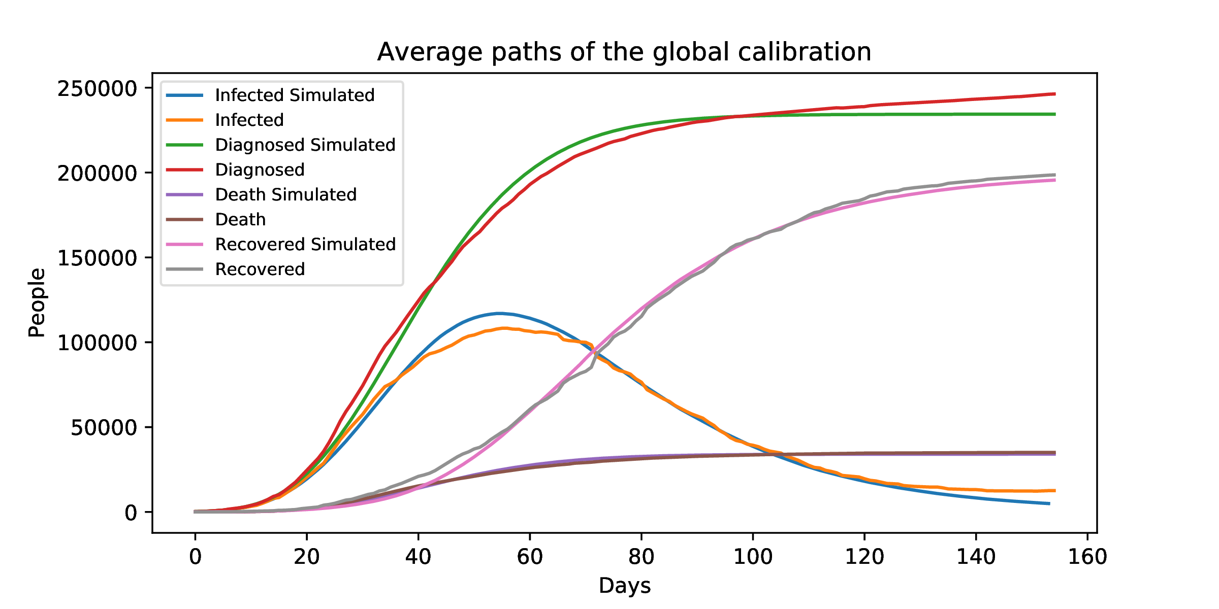
The model is calibrated in such a way the mean paths of infected, death and recovered fit the corresponding observed values, as well as the variability of , and . Our approach is not only able to adjust observed data, but also to study the different possible scenarios according to its stochastic behavior.
The paper is organized as follows. In Section 2 we present a descriptive analysis of , and corresponding to the evolution of the pandemic in Italy ( https://raw.githubusercontent.com/pcm-dpc/COVID-19/master/dati-andamento-nazionale/dpc-covid19-ita-andamento-nazionale.csv). Section 3 is devoted to present our stochastic SIRD model for the Italian COVID-19 outbreak. The model is calibrated in Section 4, while we simulate some different scenarios in Section 5. Finally, a discussion of the results and proposals of future research are presented in Section 6.
2 A descriptive analysis of the SIRD model in the Italian COVID-19 outbreak
Let us consider a stochastic SIRD model of the form
| (1) |
where denote the number of daily observed susceptible, infected, recovered and death, N is the population size and represent the rates of infection, recovery and death. As in all the data set, we consider the following simpler version of the above model
| (2) |
Now we observe the behavior of this model in Italy in the period from the 24/2/2020 to the 28/7/2020. In Figure 1 we can observe the paths of (totale positivi in the data set), (dimessi-guariti), (deceduti) and the total number of diagnosed (, totale casi).

2.1 The process
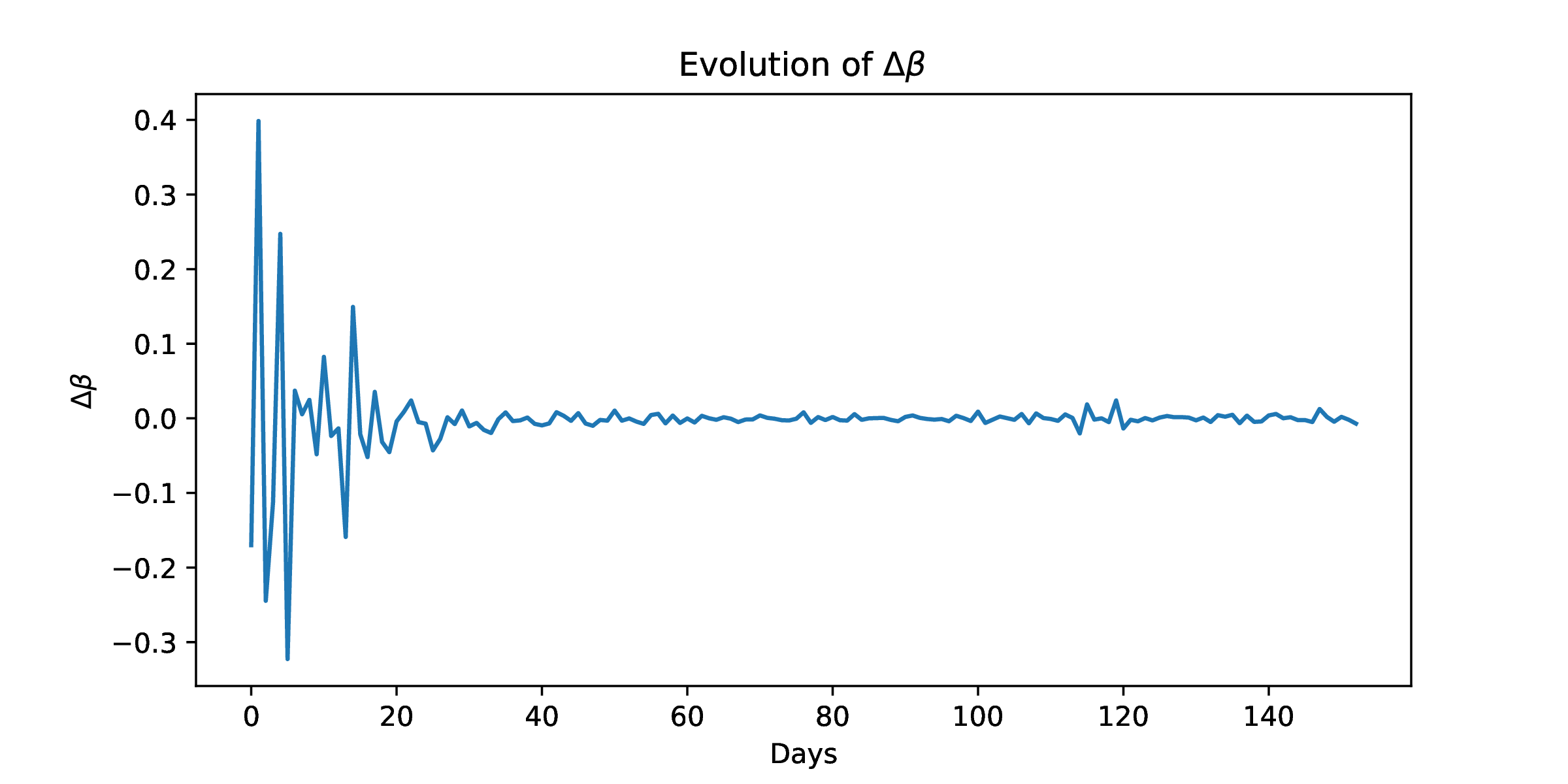
Now let us observe . In Figure 2 we can see the behavior of , that is a decreasing function of time. This fits what expected due to the lock-down, that reduced the number of contacts between individuals. In Figure 3, we can see the corresponding increments (i.e., ), that are more variable at the beginning of the sample, when is higher.

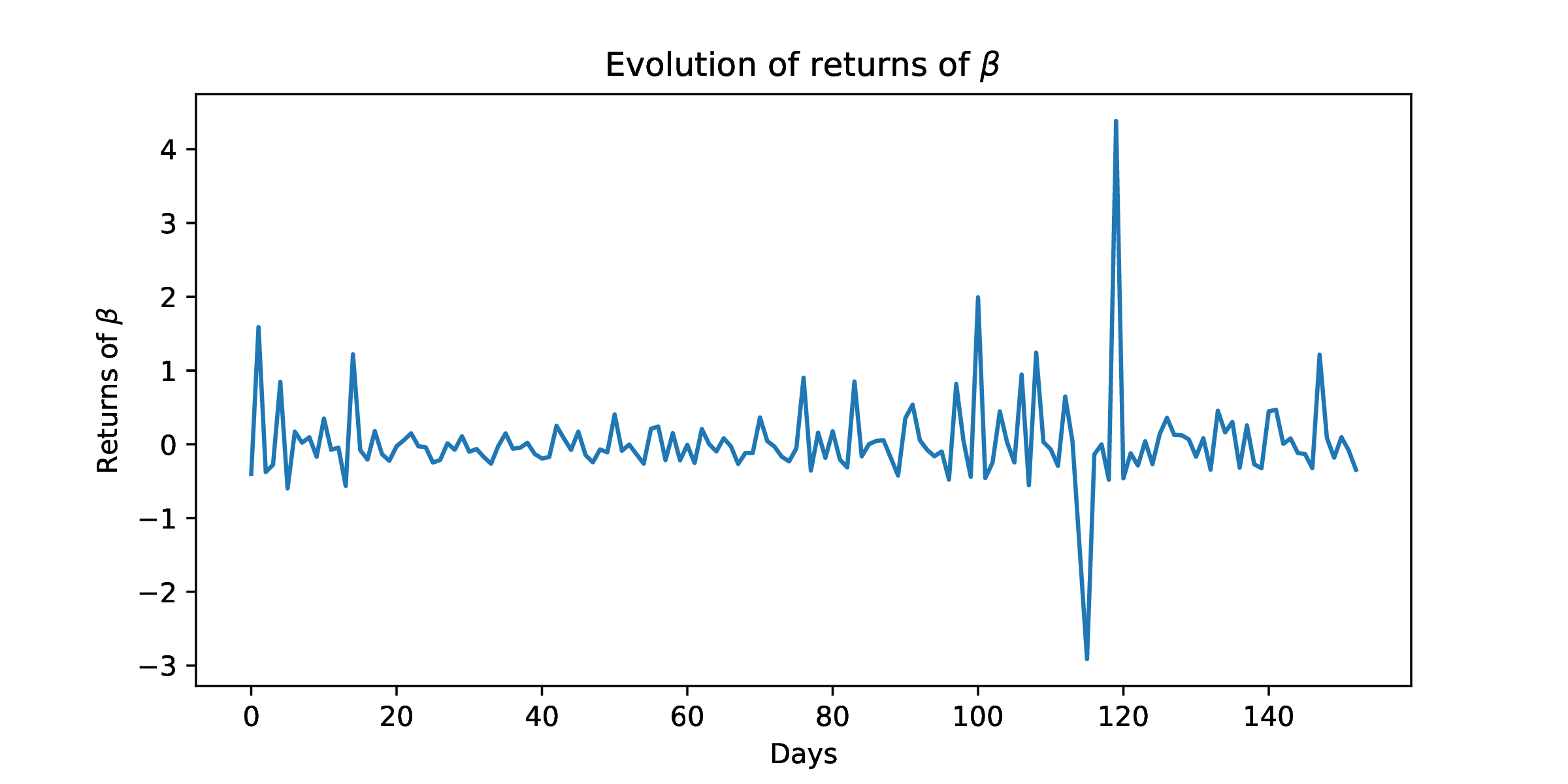
Moreover, in Figure 4 we can see the returns that have a stationary mean. After deleting the outliers at days 115 and 119 (making them equal to zero), the corresponding autocorrelation function, see Figure 5, reveals a negative correlation between increments. The empirical analysis suggests to model as a process with negative correlated increments with a decreasing mean. This process is designed in Section 3.

2.2 The process
The time behavior of can be seen in Figure 6. We observe that it is similar to the behavior of , but with a delay. Moreover, Figures 7 and 8 show a clear relationship between the daily new diagnosed and deaths, with a delay of 4 days. 11 1 This finding appears consistent with data by Istituto Superiore di Sanità https://www.epicentro.iss.it/coronavirus/bollettino/Report-COVID-2019_17_marzo-v2.pdf. In Figure 9, we can see a strong link between total diagnosed and deaths. In Figures 10 and 11 we can see that this relationship is linear. Then, as the number of new infected is given by , the daily increments of deaths () would be modeled simply as , for some positive constant . This leads to the following model for :


2.3 The process
Finally, let us observe the path of in Figure 12. This recovery rate seems to move between an upper and a lower bound, that we can interpret as the rate under stressed conditions of the health system, and the rate when this system adapts to the new scenario and the epidemic curve decays. This is connected to the approach in [1], where is assumed to be described by a logistic function, and the rate of recovery increases from a initial value and it stabilizes at some higher level.

A measure of the stress of the model can be defined as the quantity
| (3) |
where is the average of the diagnosed people the last days. If there are no new infections, the number of diagnosed remains stable, and then the above quantity is near 1. Otherwise, a high increment of new cases translates into a decrease of the value of this ratio. In Figure 13, we can see the behavior of this process

We can also observe in Figure 12 a big variance, as expected due to the fact that not everybody recovers at the same speed. Then we would like to add some noise, multiplying this time series by an adequate random factor, as we detail in the following section.
3 A stochastic SIRD model
We propose a stochastic SIRD model where randomness is embedded by modeling the parameters of infection (), mortality () and recovery (). In the following subsections, we will describe the model for each one of the parameters.
3.1 A stochastic model for .
As the return of are negatively correlated, it is natural to construct a model based on the fractional Brownian motion (fBm). The fBm is a Gaussian process with stationary increments, which depends on a parameter called the Hurst parameter. More precisely, a process is called a fractional Brownian motion (fBm) if
- •
- •
.
Except in the Brownian motion case , the fBm increments are correlated. Denote and define . Then we have
| (4) | |||||
Notice that this quantity is positive for and negative if .
Then, a natural candidate to model is given by
| (5) |
where is a fractional Brownian motion with and is a constant. Apart from the negative correlated returns, this process has also a decreasing mean, as we prove in the following result.
Proposition 3.1.
Consider a fractional Brownian motion with and the process defined by (8). Then, provided , is decreasing as .
Proof.
A recursive computation gives us that
with
where . The above product can be written as
| (6) |
Now, we can compute the expectation using Isserlis Theorem. This gives us that
where we have used that partitions exist only if is even. Then, as is positive for all even and all the are strictly negative, is decreasing. This allows us to complete the proof.
∎
Even when the model (8) reproduces some empirical properties of , a numerical analysis shows that it has to be modified before being an adequate model. More precisely, we can see in Figure 14 that the variability of the paths is high, and that the process can even become negative (see also Figure 15). Moreover, the estimated correlation between two consecutive increments of does not coincide with the observed for the returns.

A way to reduce the variance of the paths is obviously to define a model of the type
| (8) |
where are given by
being independent fractional Brownian motions with Hurst parameter and where are positive constant. The interpretation of (8) is intuitive: the observed process is really the sum of different stochastic that correspond to the particular transmission rates in different groups, locations, etc. In Figures 15 and 16we can observe, for , the behavior of the cases (where the volatility is too big), and , where the area delimited by the the maximum and minimum paths contain the observed values of .


3.2 A stochastic model for and .
As pointed out in 2, the linear relationship between diagnosed (with 4 days lag) and death, suggests modeling simply as
On the other hand, the observations in Section 2 lead to a model for of the type
for some positive constants and for some adequate Hurst parameter .
3.3 The global model
The above models for , and lead to the following stochastic SIRD model:
| (9) |
Notice that only 7 parameters have to be calibrated are , , and , ,, . We see in the following section how the set of the first three parameters , , , that define the driving processes of the model, is chosen based on empirical observations, while the last group is calibrated by means of a classical least squares method.
4 Calibration
4.1 The steps of the calibration process
The calibration procedure is as follows.
- •
In a first step, we fix reasonable values of and the Hurst parameters according to observed data, and
- •
fixed , , and , we calibrate , ,, by a least squares method.
Step 1 focuses on choosing adequate driving random processes for the model. As estimating with precision and robustness this group of parameters is not straightforward (see for example Glotter (2007)), so we simply proceed empirically. More precisely, we have seen in Section 2 that the maximum and the minimum paths in the case and envelope the observed time series. Moreover, the observed correlation of beta returns (for lag=1) is equal to , while (from a 1000 simulations sample), we estimate this quantity to be for and . This leads to choose in our model.
In order to choose , we compute the autocorrelation function of
At lag=1, this autocorrelation function is equal to . Then, taking into account Equation (4), we get a estimation of . Then we choose for the sake of simplicity.
4.2 Initial guess for , , , and global calibration
In order to be able to start the calibration of the other parameters, we will need to have an initial guess.
To find the parameter , we are going to fit the average against the realized . This gives us a value of 0.32250809.
For , as we have seen previously, we can obtain a nice estimation by doing a linear regression between the infected and death people. The slope ( 0.13904755) will be the initial guess for .
In the case of , in order to obtain the variables , , we minimize the distance between the average and the observed , as well as the distance between the standard deviation of the returns of and the observed . This gives us (0.03512639,0.5) as initial guess.
Once we have the initial guess, we find the best possible parameters to minimize the distance between the infected, the death and the recovered time series as well as the empirical variance of the by OLS.
5 Results
Following the procedure in the previous section, we get the following estimation of the parameters of the model:
5.1 The average paths of the global calibration
Simulating the model and taking the corresponding mean paths we fit the observed data, as we can see in Figure 17.
5.2 The average paths of , , and
The same analysis can be done for , , and :


5.3 Some simulated paths
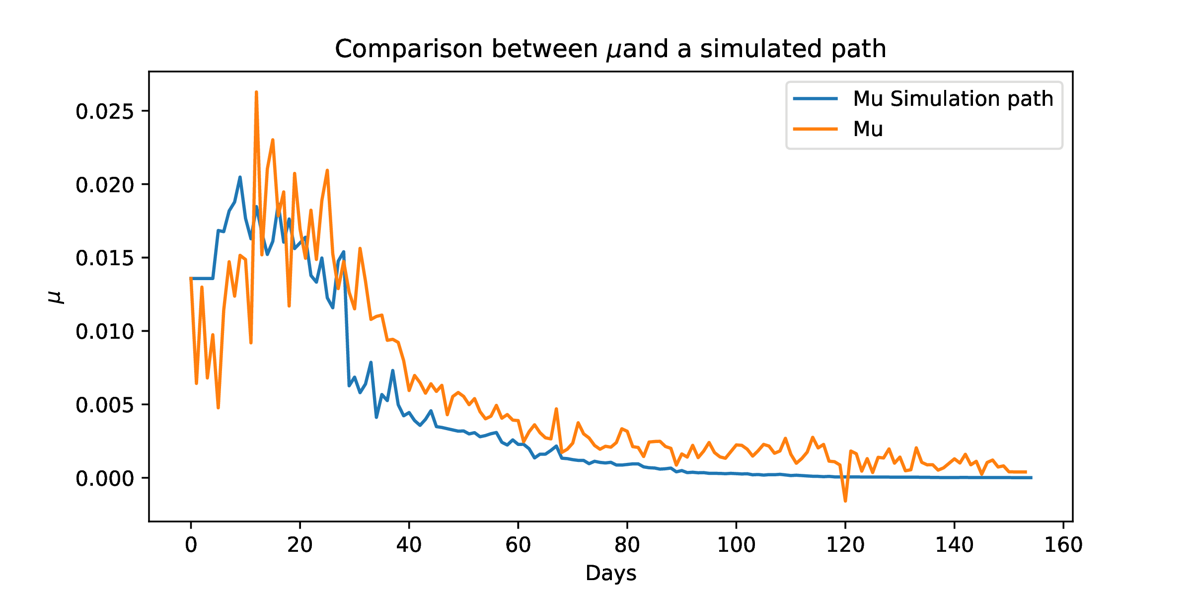
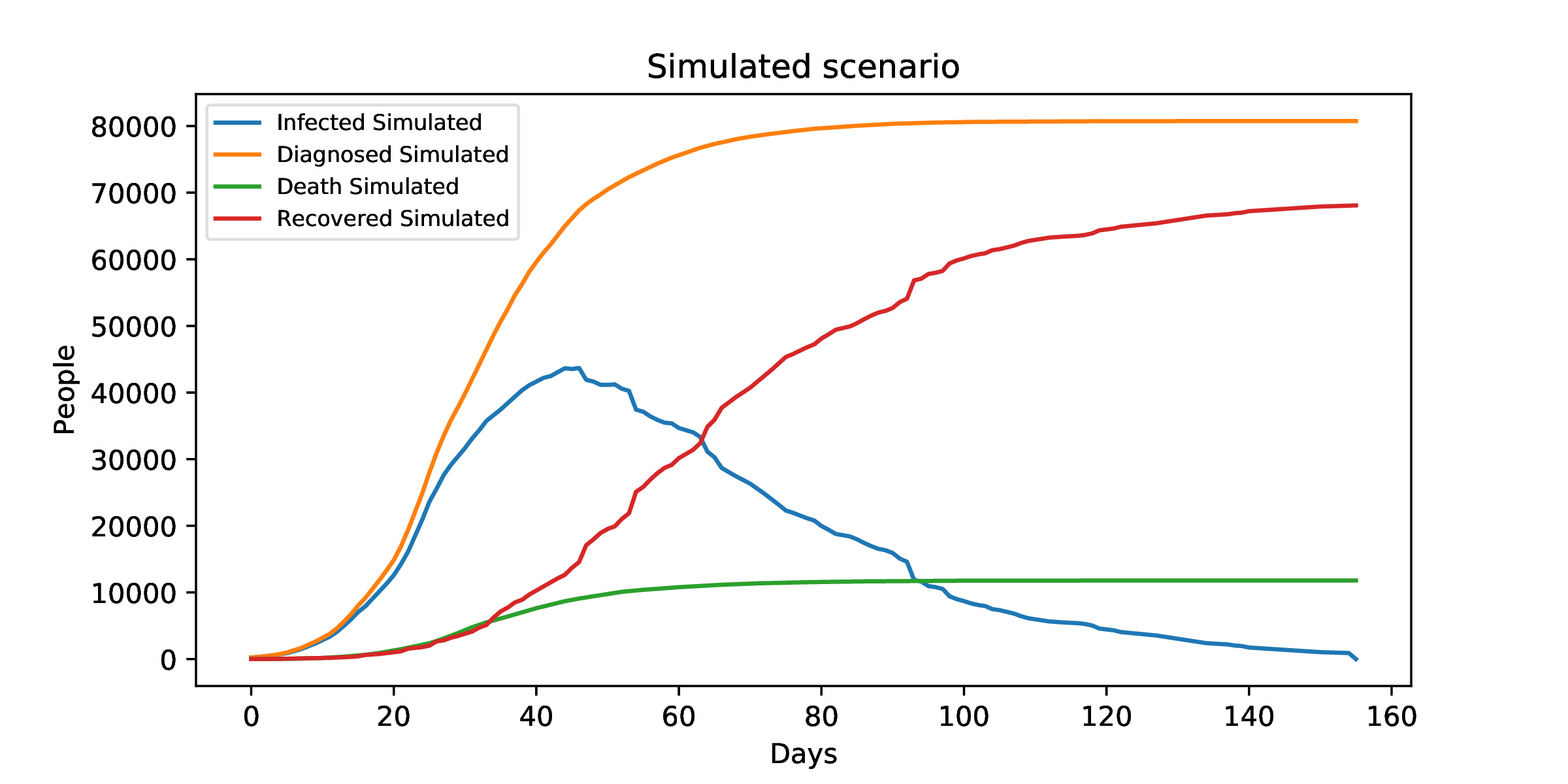
Some simulated paths for and can be observed in the following figures:


Different random scenarios can be seen in the following figures:


6 Discussion
In the present work, we have extended the classic SIRD model including stochastic parameters and we obtain an easy-to-calibrate pure probabilistic model. We have been able to reproduce the evolution of the parameters of the Italian outbreak using only seven parameters. The properties of the fractional Brownian motion and the relationship between the parameters of the model are able to reproduce the exponential and logistic trends observed for example in [1]. Therefore, we have been able to fit the empirical data as well as imitate the noise of the variables. One of the advantages of having a stochastic model is that we are capable of generating a wide variety of scenarios.
One challenging problem is now to model the evolution after a lockdown. This translates into a new dynamics of , probably driven by a fBm with . Moreover, the comparison between different countries that applied different policies during the pandemic would be of great interest.
References
- [1] D. Caccavo: Chinese and Italian COVID-19 outbreaks can be correctly described by a modified SIRD model. MedRxiv, 2020.
- [2] L. Changguo, P. Yongzhen, Z. Meixia, and D. Yue: Parameter Estimation on a Stochastic SIR Model with Media Coverage. Discrete Dynamics in Nature and Society Volume 2018, Article ID 3187807.
- [3] B. Ivorra, M. R. Ferrández, M. Vela-Pérez, A. M. Ramos: Mathematical modeling of the spread of the coronavirus disease 2019 (COVID-19) taking into account the undetected infections. The case of China. Communications in Nonlinear Science and Numerical Simulation, Vol. 88, 2020.
- [4] B. Mandelbrot, and J.W. van Ness: Fractional Brownian motions, fractional noises and applications, SIAM Review, Vol.10 (4): 422–437, 1968.
- [5] M. J. Plank, R. N. Binny, S. C. Hendy, A. Lustig , A. James, and N. Steyn: A stochastic model for COVID-19 spread and the effects of Alert Level 4 in Aotearoa New Zealand. 2020. Available at https://www.medrxiv.org/content/10.1101/2020.04.08.20058743v1
- [6] E. Platen: Stochastic Modelling of the COVID-19 Epidemic. 2020. Available at SSRN: https://ssrn.com/abstract=3586208
- [7] N. M. Yanev, V. K. Stoimenova, and D. V. Atanasov: Stochastic modeling and estimation of COVID-19 population dynamics. Available at https://arxiv.org/abs/2004.00941