跳到论文正文
W Papers独立论文阅读器 arXiv:2007.16134 论文正文 计算阅读时间 · 0%
引用这篇论文根据当前论文元数据生成,正式投稿前建议核对。


License: arXiv.org perpetual non-exclusive license
arXiv:2007.16134v1 [math.NA] 31 Jul 2020

Numerical Analysis of Backward Subdiffusion Problems

Zhengqi Zhang    Zhi Zhou Affiliation: Department of Applied Mathematics, The Hong Kong Polytechnic University, Kowloon, Hong Kong SAR, China Email: 19076082r@connect.polyu.hk and zhizhou@polyu.edu.hk
Abstract

The aim of this paper is to develop and analyze numerical schemes for approximately solving the backward problem of subdiffusion equation involving a fractional derivative in time with order α∈(0,1)\alpha\in(0,1). After using quasi-boundary value method to regularize the ”mildly” ill-posed problem, we propose a fully discrete scheme by applying finite element method (FEM) in space and convolution quadrature (CQ) in time. We provide a thorough error analysis of the resulting discrete system in both cases of smooth and nonsmooth data. The analysis relies heavily on smoothing properties of (discrete) solution operators, and nonstandard error estimate for the direct problem in terms of problem data regularity. The theoretical results are useful to balance discretization parameters, regularization parameter and noise level. Numerical examples are presented to illustrate the theoretical results.

April 2019

Keywords: fractional subdiffusion, backward problem, quasi-boundary value method, finite element method, convolution quadrature, error analysis

1 Introduction

Let Ω⊂ℝd\Omega\subset\mathbb{R}^{d} (d≥1d\geq 1) be a bounded and convex domain with smooth boundary ∂Ω\partial\Omega, and consider the following subdiffusion equation

∂tαu−Δ​u=finΩ×(0,T),u=0on∂Ω×(0,T),u⁡(0)=u0inΩ\displaystyle\eqalign{\partial_{t}^{\alpha}u-\Delta u&=f\qquad{\rm in}\,\,\,\Omega\times(0,T),\\ \qquad\quad~u&=0\qquad{\rm on}\,\,\,\partial\Omega\times(0,T),\\ \qquad~~u(0)&=u_{0}\qquad{\rm in}\,\,\,\Omega}

where T>0T>0 is a fixed terminal time, f∈L∞​(0,T,L2​(Ω))f\in L^{\infty}(0,T;L^{2}(\Omega)) and u0∈L2​(Ω)u_{0}\in L^{2}(\Omega) are given source term and initial data, respectively, and Δ\Delta is the Laplace operator in space. Here ∂tαu⁡(t){\partial_{t}^{\alpha}}u(t) denotes the Caputo fractional derivative in time tt of order α∈(0,1)\alpha\in(0,1):

∂tαu⁡(t)=1Γ⁡(1−α)​∫0t(t−s)−α​u′​(s)​𝑑s.\displaystyle{\partial_{t}^{\alpha}}u(t)=\frac{1}{\Gamma(1-\alpha)}\int_{0}^{t}(t-s)^{-\alpha}u^{\prime}(s){\rm d}s.

In recent years, there has been a growing interest in the mathematical and numerical analysis of subdiffusion models due to their diverse applications in describing subdiffusion processes arising from physics, engineering, biology and finance. In a subdiffusion process, the mean squared particle displacement grows only sublinearly with time, instead of growing linearly with time as in the normal diffusion process. We refer interested readers to [14, 15] for a long list of applications of subdiffusion arising from biology and physics.

Inverse problems for fractional diffusion have attracted much interest, and there has already been a vast literature; see e.g., review papers [7, 9, 10, 12] and references therein. In this paper, we aim at the classical backward problem, i.e., determining the function u⁡(x,t)u(x,t) with (x,t)∈Ω×[0,T)(x,t)\in\Omega\times[0,T) from a terminal observation

u⁡(x,T)=g⁡(x),for allx∈Ω.u(x,T)=g(x),\qquad\mbox{for all}\quad x\in\Omega.

With f≡0f\equiv 0, the subdiffusion model (1) has the following smoothing property [16]:

c1​‖u0‖L2​(Ω)≤‖u⁡(T)‖H2​(Ω)≤c2​‖u0‖L2​(Ω).c_{1}\|u_{0}\|_{L^{2}(\Omega)}\leq\|u(T)\|_{H^{2}(\Omega)}\leq c_{2}\|u_{0}\|_{L^{2}(\Omega)}.

This property contrasts sharply with the classical parabolic counterpart (α=1\alpha=1), whose solution is infinitely differentiable in space for all t>0t>0. Thus, the backward problem of subdiffusion is far “less” ill-posed than that of normal diffusion. The existence, uniqueness and stability of the time-fractional backward problem were analyzed by Sakamoto and Yamamoto in [16]. This work motivates many subsequent developments of regularized algorithms. In [11], Liu and Yamamoto proposed a numerical method based on the quasi-reversibility method, and analyze the approximation error (in terms of noise level) under a priori smoothness assumption on u0u_{0}. Then a total variation regularization method was proposed and studied by Wang and Liu in [21]. In [20], Wang and Wei developed and analyzed an iteration method to regularize the backward problem. The quasi-boundary value method for solving the fractional backward problem was firstly studied in [23] for a one-dimensional subdiffusion model, and then extended in [22] to the general case by modifying the regularization term. See also [2] for a novel Hölder type estimate of the quasi-boundary value methods.

To solve the regularized system, people applied different numerical approaches, e.g., finite element method, finite different method, etc. Then some discretization error will be introduced into the system. Therefore it is necessary to establish an estimate to balance discretization parameter, regularization parameter and noise level. However, such an analysis remains unavailable, and it is precisely this gap that the project aims to fill in.

Specifically, we assume that the observation data gδg^{\delta} is noisy such that

‖gδ−g‖L2​(Ω)≤δ.\|g^{\delta}-g\|_{L^{2}(\Omega)}\leq\delta.

To regularize the ill-posed problem, we apply the quasi-boundary value method [2, 23] and consider

∂tαu~δ−Δ​u~δ=f.in​Ω×(0,T),u~δ=0on∂Ω×(0,T),γ​u~δ​(0)+u~δ​(T)=gδinΩ,\displaystyle\eqalign{~\quad\partial_{t}^{\alpha}\tilde{u}^{\delta}-\Delta\tilde{u}^{\delta}&=f.\qquad\mbox{in}\,\,\,\Omega\times(0,T),\\ \qquad\quad\qquad\tilde{u}^{\delta}&=0\qquad\mbox{on}\,\,\,\partial\Omega\times(0,T),\\ \gamma\tilde{u}^{\delta}(0)+\tilde{u}^{\delta}(T)&=g_{\delta}\qquad\mbox{in}\,\,\,\Omega,\\ }

where γ>0\gamma>0 denotes the regularization parameter. In [23], Yang and Liu considered the homogeneous problem (f≡0f\equiv 0). It was proved that the regularized problem (1) has a unique solution, and if u0∈L2​(Ω)u_{0}\in L^{2}(\Omega), then for all t∈[0,T]t\in[0,T] there holds

‖(u~δ−u)​(t)‖L2​(Ω)→0,asγ,δ→0​and​δγ→0.\displaystyle\|(\tilde{u}^{\delta}-u)(t)\|_{L^{2}(\Omega)}\rightarrow 0,\quad\mbox{as}\quad\gamma,\delta\rightarrow 0~~\mbox{and}~~\frac{\delta}{\gamma}\rightarrow 0. (1.9)

Moreover, if u0∈Dom​(A)=H2​(Ω)∩H01​(Ω)u_{0}\in\mbox{Dom}(A)=H^{2}(\Omega)\cap H_{0}^{1}(\Omega), there holds

‖(u~δ−u)​(t)‖C⁡([0,T],L2​(Ω))≤c​δ​γ−1,\displaystyle\|(\tilde{u}^{\delta}-u)(t)\|_{C([0,T];L^{2}(\Omega))}\leq c\delta\gamma^{-1},

where the constant cc depends only on u0u_{0}, gg, gδg_{\delta}, but is independent of δ\delta and γ\gamma. By choosing γ=O⁡(δ)\gamma=O(\sqrt{\delta}) a priori, one obtains an approximation with accuracy O⁡(δ)O(\sqrt{\delta}). The result contrasts sharply with that for normal diffusion, and the proof relies on the linear-decay property of the Mittag-Leffler function Eα,1​(−x)E_{\alpha,1}(-x).

To numerically solve the backward subdiffusion problem, we discretize the regularized problem (1) by applying piecewise linear finite element method (FEM) in space and convolution quadrature generated by backward Euler scheme (CQ-BE) in time. We provide thorough error analysis of proposed scheme and specify the way to balance the discrization error, regularization parameter and noise level. For example, we let hh be the spatial mesh size and τ\tau be temporal step size. Suppose u⁡(t)u(t) is the exact solution of the backward subdiffusion problem and U~nδ\tilde{U}^{\delta}_{n} is the fully discrete solution (which approximates the exact solution at tn=n​τt_{n}=n\tau). Then we prove that if u0∈L2​(Ω)u_{0}\in L^{2}(\Omega), then with ℓh=max⁡(1,|ln⁡h|)\ell_{h}=\max(1,|\ln h|), there holds (Theorem 4.1 (ii))

‖U~0δ−u⁡(0)‖L2​(Ω)→0,as​γ→0,δγ→0,h​ℓh12γ→0​and​τ12γ→0.\displaystyle\hskip-20.0pt\|\tilde{U}_{0}^{\delta}-u(0)\|_{L^{2}(\Omega)}\rightarrow 0,\quad\mbox{as}~~\gamma\rightarrow 0,~\frac{\delta}{\gamma}\rightarrow 0,~\frac{h\ell_{h}^{\frac{1}{2}}}{\gamma}\rightarrow 0~\mbox{and}~\frac{\tau^{\frac{1}{2}}}{\gamma}\rightarrow 0.

Besides, for n≥1n\geq 1, there holds (Theorem 4.1)

‖U~nδ−u⁡(tn)‖L2​(Ω)≤c⁡(γ​tn−α+(δ+γ−1​(h2​ℓh+τ))​min⁡(γ−1,tn−α)+γ−1​τ​tnα−1).\displaystyle\hskip-50.0pt\|\tilde{U}_{n}^{\delta}-u(t_{n})\|_{L^{2}(\Omega)}\leq c\Big(\gamma t_{n}^{-\alpha}+\big(\delta+\gamma^{-1}(h^{2}\ell_{h}+\tau)\big)\min(\gamma^{-1},t_{n}^{-\alpha})+\gamma^{-1}\tau t_{n}^{\alpha-1}\Big).

where the constant cc is independent of hh, τ\tau, γ\gamma and δ\delta. Then by choosing a priori h​ℓh12=O⁡(δ)h\ell_{h}^{\frac{1}{2}}=O(\delta), τ=O⁡(δ2)\tau=O(\delta^{2}) and γ=O⁡(δ)\gamma=O(\delta), one obtains an approximation with accuracy O⁡(δ)O(\delta) for all t∈(0,T]t\in(0,T], even though the approximation at t=0t=0 has no convergence rate. The analysis relies heavily on smoothing properties of (discrete) solution operators, and nonstandard error estimate for the direct problem in terms of problem data regularity [4, 5, 6]. Such the estimates could be improved provided that the problem data is smoother and compatible with the boundary condition. For instance, if u0∈H2​(Ω)∩H01​(Ω)u_{0}\in H^{2}(\Omega)\cap H_{0}^{1}(\Omega), there holds (Theorem 4.1 (i))

∥U~nδ−u(tn)∥L2​(Ω)≤c{γ+(h2+τ+δ)​min⁡(γ−1,tn−α)+τ​tnα−1,n≥1;γ+(h2+τ+δ)​γ−1,n=0.\displaystyle\hskip-36.135pt\|\tilde{U}_{n}^{\delta}-u(t_{n})\|_{L^{2}(\Omega)}\leq c\left\{\eqalign{&\gamma+(h^{2}+\tau+\delta)\min(\gamma^{-1},t_{n}^{-\alpha})+\tau t_{n}^{\alpha-1},n\geq 1;\\ &\gamma+(h^{2}+\tau+\delta)\gamma^{-1},\qquad n=0.}\right.

As far as we know, this is the first work providing rigorous error analysis of numerical methods for solving the time-fractional backward problem.

The rest of the paper is organized as follows. In Section 2, we provide some preliminary results about the solution representation and the regularization at the continuous level, which will be intensively used in error estimation. Then in Section 3 and Section 4, we describe and analyze spatially semi-discrete scheme and fully discrete scheme, respectively. Finally, in Section 5, we present illustrative numerical examples to illustrate the theoretical analysis. Throughout, the notation cc denotes a generic constant, which may change at each occurrence, but it is always independent of the noise level δ\delta, the regularization parameter γ\gamma, the mesh size hh and time step size τ\tau etc.

2 Preliminary

2.1 Solution representation and Mittag-Leffler functions

In this section, we recall the representation of the solution to the subdiffusion problem (1), which plays a key role in the analysis.

To begin with, we introduce some notation. For q≥0q\geq 0, we denote by H˙q​(Ω)\dot{H}^{q}(\Omega) the Hilbert space induced by the norm:

‖v‖H˙q​(Ω)2=∑j=1∞λjq​(v,φj)2\|v\|_{\dot{H}^{q}(\Omega)}^{2}=\sum_{j=1}^{\infty}\lambda_{j}^{q}(v,\varphi_{j})^{2}

with {λj}j=1∞\{\lambda_{j}\}_{j=1}^{\infty} and {φj}j=1∞\{\varphi_{j}\}_{j=1}^{\infty} being respectively the eigenvalues and the L2​(Ω)L^{2}(\Omega)-orthonormal eigenfunctions of the negative Laplacian −Δ-\Delta on the domain Ω\Omega with a homogeneous Dirichlet boundary condition. Then {φj}j=1∞\{\varphi_{j}\}_{j=1}^{\infty} forms orthonormal basis in L2​(Ω)L^{2}(\Omega). Further, ‖v‖H˙0​(Ω)=‖v‖L2​(Ω)=(v,v)1/2\|v\|_{\dot{H}^{0}(\Omega)}=\|v\|_{L^{2}(\Omega)}=(v,v)^{1/2} is the norm in L2​(Ω)L^{2}(\Omega). Besides, it is easy to verify that ‖v‖H˙1​(Ω)=‖∇v‖L2​(Ω)\|v\|_{\dot{H}^{1}(\Omega)}=\|\nabla v\|_{L^{2}(\Omega)} is also the norm in H01​(Ω)H_{0}^{1}(\Omega) and ‖v‖H˙2​(Ω)=‖Δ​v‖L2​(Ω)\|v\|_{\dot{H}^{2}(\Omega)}=\|\Delta v\|_{L^{2}(\Omega)} is equivalent to the norm in H2​(Ω)∩H01​(Ω)H^{2}(\Omega)\cap H^{1}_{0}(\Omega) [19, Section 3.1].

Now we represent the solution to problem (2.2) using the eigenpairs {λj,φj}j=1∞\{\lambda_{j},\varphi_{j}\}_{j=1}^{\infty}. To this end, we define solution operators F⁡(t)F(t) and E⁡(t)E(t) from [4],

F⁡(t)​χ=∑j=1∞Eα,1​(−λj​tα)​(χ,φj)​φjandE⁡(t)​χ=∑j=1∞tα−1​Eα,α​(−λj​tα)​(χ,φj)​φj,\displaystyle\hskip-54.2025ptF(t)\chi=\sum_{j=1}^{\infty}E_{\alpha,1}(-\lambda_{j}t^{\alpha})(\chi,\varphi_{j})\varphi_{j}\quad\mbox{and}\quad E(t)\chi=\sum_{j=1}^{\infty}t^{\alpha-1}E_{\alpha,\alpha}(-\lambda_{j}t^{\alpha})(\chi,\varphi_{j})\varphi_{j},\,\,\,\, (2.1)

where Eα,β​(z)E_{\alpha,\beta}(z) is the two-parameter Mittag-Leffler function:

Eα,β​(z)=∑k=0∞zkΓ⁡(k​α+β)∀z∈ℂ.E_{\alpha,\beta}(z)=\sum_{k=0}^{\infty}\frac{z^{k}}{\Gamma(k\alpha+\beta)}\quad\forall z\in\mathbb{C}. (2.2)

Then the solution of the forward problem (1) could be written as

u⁡(t)=F⁡(t)​u0+∫0tE⁡(t−s)​f​(s)​𝑑s.u(t)=F(t)u_{0}+\int_{0}^{t}E(t-s)f(s)ds. (2.3)

The Mittag-Leffler function Eα,β​(z)E_{\alpha,\beta}(z) is a generalization of the familiar exponential function eze^{z} appearing in normal diffusion. Then following decay behavior of Eα,β​(z)E_{\alpha,\beta}(z) is crucial to the smoothing properties of F⁡(t)F(t) and E⁡(t)E(t): for any α∈(0,1)\alpha\in(0,1), the function Eα,1​(−λ​tα)E_{\alpha,1}(-\lambda t^{\alpha}) decays only polynomially like t−αt^{-\alpha} as t→∞t\to\infty (cf. Lemma 2.1), which contrasts sharply with the exponential decay for e−λ​te^{-\lambda t} appearing in normal diffusion.

Note that w⁡(t)=Eα,1​(−λ​tα)w(t)=E_{\alpha,1}(-\lambda t^{\alpha}) be the solution to the initial value problem

∂tαw⁡(t)+λ​w​(t)=0,withw⁡(0)=1.{\partial_{t}^{\alpha}}w(t)+\lambda w(t)=0,\quad\mbox{with}\quad w(0)=1.

By means of Laplace transform, it can be written as

w⁡(t)=Eα,1​(−λ​tα)=12​π​i​∫Γθ,σez​t​zα−1​(zα+λ)−1​𝑑z.w(t)=E_{\alpha,1}(-\lambda t^{\alpha})=\frac{1}{2\pi\mathrm{i}}\int_{\Gamma_{\theta,\sigma}}e^{zt}z^{\alpha-1}(z^{\alpha}+\lambda)^{-1}\,dz. (2.4)

with integration over a contour Γθ,σ\Gamma_{\theta,\sigma} in the complex plane ℂ\mathbb{C} (oriented counterclockwise), defined by

Γθ,σ={z∈ℂ:|z|=δ,|argz|≤θ}∪{z∈ℂ:z=ρe±i​θ,ρ≥σ}.\Gamma_{\theta,\sigma}=\left\{z\in\mathbb{C}:|z|=\delta,|\arg z|\leq\theta\right\}\cup\{z\in\mathbb{C}:z=\rho e^{\pm\mathrm{i}\theta},\rho\geq\sigma\}.

Throughout, we fix θ∈(π2,π)\theta\in(\frac{\pi}{2},\pi) so that zα∈Σα,θ⊂Σθ:={0≠z∈ℂ:arg⁡(z)≤θ},z^{\alpha}\in\Sigma_{\alpha,\theta}\subset\Sigma_{\theta}:=\{0\neq z\in\mathbb{C}:{\rm arg}(z)\leq\theta\}, for all z∈Σθz\in\Sigma_{\theta}.

The next lemma provides the upper and lower bounds of Mittag–Leffler functions (2.2). See [18, Theorem 4] for detailed proof.

Lemma 2.1.

Assume that α∈(0,1)\alpha\in(0,1). Then there holds that

11+Γ⁡(1−α)​z≤Eα,1​(−z)≤11+Γ​(1+α)−1​z,for all​z≥0.\frac{1}{1+\Gamma(1-\alpha)z}\leq E_{\alpha,1}(-z)\leq\frac{1}{1+\Gamma(1+\alpha)^{-1}z},\quad\mbox{for all}\,\,~z\geq 0.

These important bounds directly translate into the limited smoothing property in both space and time for the solution operators E⁡(t)E(t) and F⁡(t)F(t). Next, we state a few regularity results. The proof of these results can be found in, e.g., [1, 16, 6].

Theorem 2.1.

Let u⁡(t)u(t) be defined in (2.3). Then the following statements hold.

  • (i)\rm(i)

    If u0∈H˙q​(Ω)u_{0}\in\dot{H}^{q}(\Omega) with s∈[0,2]s\in[0,2] and f=0f=0, then u⁡(t)u(t) is the solution to problem (1), and u⁡(t)u(t) satisfies

    ‖∂t(m)u⁡(t)‖H˙p​(Ω)≤c​t(s−p)​α2−m​‖u0‖H˙q​(Ω)\|\partial_{t}^{(m)}u(t)\|_{\dot{H}^{p}(\Omega)}\leq ct^{\frac{(s-p)\alpha}{2}-m}\|{u_{0}}\|_{\dot{H}^{q}(\Omega)}

    with 0≤p−q≤20\leq p-q\leq 2 and any integer m≥0m\geq 0 .

  • (ii)\rm(ii)

    If u0=0u_{0}=0 and f∈Lp​(0,T,L2​(Ω))f\in L^{p}(0,T;L^{2}(\Omega)) with 1<p<∞1<p<\infty, then there holds

    ‖u‖Lp​(0,T,H˙2​(Ω))+‖∂tαu‖Lp​(0,T,L2​(Ω))≤c​‖f‖Lp​(0,T,L2​(Ω)).\|u\|_{L^{p}(0,T;\dot{H}^{2}(\Omega))}+\|{\partial_{t}^{\alpha}}u\|_{L^{p}(0,T;L^{2}(\Omega))}\leq c\|f\|_{L^{p}(0,T;L^{2}(\Omega))}.

    Moreover, if f∈Lp​(0,T,L2​(Ω))f\in L^{p}(0,T;L^{2}(\Omega)) with 1/α<p<∞1/\alpha<p<\infty, then u⁡(t)u(t) is the solution to problem (1) such that u∈C⁡([0,T],L2​(Ω))u\in C([0,T];L^{2}(\Omega)).

2.2 Reformulation of original problem

In our paper, we shall study an equivalent reformulation of the original backward subdiffusion problem (1). We let w⁡(t)=u⁡(t)−∫0tE⁡(t−s)​f​(s)​𝑑sw(t)=u(t)-\int_{0}^{t}E(t-s)f(s)\,ds, then ww satisfies the subdiffusion problem (1) with trivial source term, and the terminal data is

w⁡(T)=u⁡(T)−∫0TE⁡(T−s)​f​(s)​𝑑s.w(T)=u(T)-\int_{0}^{T}E(T-s)f(s)\,ds.

Meanwhile, in case that f∈Lp​(0,T,L2​(Ω))f\in L^{p}(0,T;L^{2}(\Omega)) with 1/α<p<∞1/\alpha<p<\infty, then by Theorem 2.1 we have w⁡(0)=u⁡(0)=u0w(0)=u(0)=u_{0}. Then without loss of generality, we only consider the following backward subdiffusion problem with trivial source data:

∂tαu−Δ​u=0inΩ×(0,T),u=0on∂Ω×(0,T),u⁡(T)=ginΩ.\displaystyle\eqalign{\partial_{t}^{\alpha}u-\Delta u&=0\qquad\mbox{in}\,\,\,\Omega\times(0,T),\\ \qquad\quad~u&=0\qquad\mbox{on}\,\,\,\partial\Omega\times(0,T),\\ \qquad~u(T)&=g\qquad\mbox{in}\,\,\,\Omega.\\ }

The solution uu has the representation that

u⁡(t)=F⁡(t)​u​(0)=F⁡(t)​(F​(T)−1​g).u(t)=F(t)u(0)=F(t)(F(T)^{-1}g). (2.9)

Inspired by the quasi-boundary value method discussed in [2, 23], we defined an axillary function u~​(t)\tilde{u}(t), which satisfies the regularized problem (without noise):

∂tαu~​(t)−Δ​u~​(t)=0,in​Ω×(0,T),u~=0on∂Ω×(0,T),γ​u~​(0)+u~​(T)=g,in​Ω.\displaystyle\eqalign{{\partial_{t}^{\alpha}}\tilde{u}(t)-\Delta\tilde{u}(t)&=0,\qquad\mbox{in}\,\,\,\Omega\times(0,T),\\ \qquad\qquad\quad\tilde{u}&=0\qquad\mbox{on}\,\,\,\partial\Omega\times(0,T),\\ ~~\gamma\tilde{u}(0)+\tilde{u}(T)&=g,\qquad\mbox{in}\,\,\,\Omega.}

Here γ\gamma denotes the regularization parameter. The appearance of regularization term essentially improves the regularity of the backward problem.

Analogue to (2.9), the function u~\tilde{u} can be represented by

u~​(t)=F⁡(t)​u~​(0)=F⁡(t)​(γ​I+F⁡(T))−1​g=F⁡(t)​(γ​I+F⁡(T))−1​(F⁡(T)​u0),\hskip-35.0pt\tilde{u}(t)=F(t)\tilde{u}(0)=F(t)\big(\gamma I+F(T)\big)^{-1}g=F(t)\big(\gamma I+F(T)\big)^{-1}\big(F(T)u_{0}\big), (2.14)

where II denotes the identity operator.

The next lemma provides an estimate of the operator F⁡(t)​(γ​I+F⁡(T))−1F(t)\big(\gamma I+F(T)\big)^{-1}.

Lemma 2.2.

Let F⁡(t)F(t) be operator defined in (2.1), then

‖F⁡(t)​(γ​I+F⁡(T))−1​v‖H˙q​(Ω)≤c​min⁡(γ−1,t−α)​‖v‖H˙q​(Ω)∀q≥0,\|F(t)\big(\gamma{I}+F(T)\big)^{-1}v\|_{\dot{H}^{q}(\Omega)}\leq c\min(\gamma^{-1},t^{-\alpha})\|v\|_{\dot{H}^{q}(\Omega)}\quad\forall~q\geq 0,

where the generic constant cc may depends on TT, but is always independent of γ\gamma and tt.

Proof.

From Lemma 2.1 we have Eα,1​(−z)>0E_{\alpha,1}(-z)>0 for any z≥0z\geq 0, then

‖F⁡(t)​(γ​I+F⁡(T))−1​v‖H˙q​(Ω)2=∑j=1∞[Eα,1​(−λj​tα)γ+Eα,1​(−λj​Tα)]2​λjq​(v,φj)2.\eqalign{\|F(t)\big(\gamma{I}+F(T)\big)^{-1}v\|_{\dot{H}^{q}(\Omega)}^{2}&=\sum_{j=1}^{{\infty}}\left[\frac{E_{\alpha,1}(-\lambda_{j}t^{\alpha})}{\gamma+E_{\alpha,1}(-\lambda_{j}T^{\alpha})}\right]^{2}\lambda_{j}^{q}(v,\varphi_{j})^{2}.}

By applying the fact that 0≤Eα,1​(−z)≤10\leq E_{\alpha,1}(-z)\leq 1 with z≥0z\geq 0, we arrive at

‖F⁡(t)​(γ​I+F⁡(T))−1​v‖H˙q​(Ω)2≤γ−1​‖v‖H˙q​(Ω)2.\|F(t)\big(\gamma{I}+F(T)\big)^{-1}v\|_{\dot{H}^{q}(\Omega)}^{2}\leq\gamma^{-1}\|v\|_{\dot{H}^{q}(\Omega)}^{2}.

On the other hand, we apply Lemma 2.1 again to obtain for any t∈(0,T]t\in(0,T]

Eα,1​(−λj​tα)γ+Eα,1​(−λj​Tα)\displaystyle\frac{E_{\alpha,1}(-\lambda_{j}t^{\alpha})}{\gamma+E_{\alpha,1}(-\lambda_{j}T^{\alpha})} ≤Eα,1​(−λj​tα)Eα,1​(−λj​Tα)≤1+Γ⁡(1−α)​(λj​Tα)1+Γ​(1+α)−1​(λj​tα)\displaystyle\leq\frac{E_{\alpha,1}(-\lambda_{j}t^{\alpha})}{E_{\alpha,1}(-\lambda_{j}T^{\alpha})}\leq\frac{1+\Gamma(1-\alpha)(\lambda_{j}T^{\alpha})}{1+\Gamma(1+\alpha)^{-1}(\lambda_{j}t^{\alpha})}
≤1+Γ⁡(1−α)​(λj​Tα)Γ​(1+α)−1​(λj​tα)≤cT​t−α.\displaystyle\leq 1+\frac{\Gamma(1-\alpha)(\lambda_{j}T^{\alpha})}{\Gamma(1+\alpha)^{-1}(\lambda_{j}t^{\alpha})}\leq c_{T}t^{-\alpha}.

and hence

‖F⁡(t)​(γ​I+F⁡(T))−1​v‖H˙q​(Ω)≤c​t−α​‖v‖H˙q​(Ω).\|F(t)\big(\gamma{I}+F(T)\big)^{-1}v\|_{\dot{H}^{q}(\Omega)}\leq ct^{-\alpha}\|v\|_{\dot{H}^{q}(\Omega)}.

This completes the proof of the lemma.

Using this lemma, we can derive the following estimate of u~​(t)−u​(t)\tilde{u}(t)-u(t) with t∈[0,T)t\in[0,T).

Lemma 2.3.

Let uu and u~\tilde{u} be solutions to problems (2.2) and (2.2), respectively. Then there holds

‖u~​(0)−u⁡(0)‖L2​(Ω)≤c​γq2​‖u0‖H˙q​(Ω)∀q∈[0,2].\|\tilde{u}(0)-u(0)\|_{L^{2}(\Omega)}\leq c\gamma^{\frac{q}{2}}\|u_{0}\|_{\dot{H}^{q}(\Omega)}\qquad\forall~q\in[0,2].

Meanwhile, for any t∈(0,T)t\in(0,T), there holds

‖u~​(t)−u⁡(t)‖L2​(Ω)≤c​γ​t−(1−q2)​α​‖u0‖H˙q​(Ω)∀q∈[0,2].\|\tilde{u}(t)-u(t)\|_{L^{2}(\Omega)}\leq c\gamma t^{-(1-\frac{q}{2})\alpha}\|u_{0}\|_{\dot{H}^{q}(\Omega)}\qquad\forall~q\in[0,2].

where the generic constant cc may depends on TT, but is always independent of γ\gamma and tt.

Proof.

By (2.9) and (2.14) we obtain

u~​(0)−u⁡(0)=−(γ​I+F⁡(T))−1​γ​u0.\tilde{u}(0)-u(0)=-\big(\gamma I+F(T)\big)^{-1}\gamma u_{0}.

Now applying (2.1) and positivity of Eα,1​(z)E_{\alpha,1}(z) with z≤0z\leq 0, we derive that for any q∈[0,2]q\in[0,2],

‖u~​(0)−u⁡(0)‖L2​(Ω)2=‖(γ​I+F⁡(T))−1​γ​u0‖L2​(Ω)2=∑j=1∞(γγ+Eα,1​(−λj​Tα))2​(u0,φj)2≤∑j=1∞γqλjq​|Eα,1​(−λj​Tα)|q​λjq​(u0,φj)2.\eqalign{\|\tilde{u}(0)-u(0)\|_{L^{2}(\Omega)}^{2}&=\|(\gamma I+F(T))^{-1}\gamma u_{0}\|_{L^{2}(\Omega)}^{2}\\ &=\sum_{j=1}^{\infty}\Big(\frac{\gamma}{\gamma+E_{\alpha,1}(-\lambda_{j}T^{\alpha})}\Big)^{2}(u_{0},\varphi_{j})^{2}\\ &\leq\sum_{j=1}^{\infty}\frac{\gamma^{q}}{\lambda_{j}^{q}|E_{\alpha,1}(-\lambda_{j}T^{\alpha})|^{q}}\lambda_{j}^{q}(u_{0},\varphi_{j})^{2}.}

The property of Mittag-Leffler functions in Lemma 2.1 implies that

γqλjq​|Eα,1​(−λj​Tα)|q≤c​γq​(1+λj​T)qλjq≤cT​γq.\frac{\gamma^{q}}{\lambda_{j}^{q}|E_{\alpha,1}(-\lambda_{j}T^{\alpha})|^{q}}\leq\frac{c\gamma^{q}(1+\lambda_{j}T)^{q}}{\lambda_{j}^{q}}\leq c_{T}\gamma^{q}.

and hence

‖u~​(0)−u⁡(0)‖L2​(Ω)2≤c​γq​‖u0‖H˙q​(Ω)2.\|\tilde{u}(0)-u(0)\|_{L^{2}(\Omega)}^{2}\leq c\gamma^{q}\|u_{0}\|_{\dot{H}^{q}(\Omega)}^{2}.

Now we turn to the second estimate, which follows from the representation

u~​(t)−u⁡(t)=−F⁡(t)​(γ​I+F⁡(T))−1​γ​u0.\tilde{u}(t)-u(t)=-F(t)\big(\gamma I+F(T)\big)^{-1}\gamma u_{0}.

Here we apply the definition of the solution operator and obtain

‖u~​(t)−u⁡(t)‖L2​(Ω)2=‖F⁡(t)​(γ​I+F⁡(T))−1​γ​u0‖L2​(Ω)2=∑j=1∞(γ​Eα,1​(−λj​tα)γ+Eα,1​(−λj​Tα))2​(u0,φj)2≤γ2​∑j=1∞(Eα,1​(−λj​tα)λjq/2​Eα,1​(−λj​Tα))2​λjq​(u0,φj)2\eqalign{\|\tilde{u}(t)-u(t)\|_{L^{2}(\Omega)}^{2}&=\|{F(t)}(\gamma I+F(T))^{-1}\gamma u_{0}\|_{L^{2}(\Omega)}^{2}\\ &=\sum_{j=1}^{\infty}\left(\frac{\gamma E_{\alpha,1}(-\lambda_{j}t^{\alpha})}{\gamma+E_{\alpha,1}(-\lambda_{j}T^{\alpha})}\right)^{2}(u_{0},\varphi_{j})^{2}\\ &\leq\gamma^{2}\sum_{j=1}^{\infty}\left(\frac{E_{\alpha,1}(-\lambda_{j}t^{\alpha})}{\lambda_{j}^{q/2}E_{\alpha,1}(-\lambda_{j}T^{\alpha})}\right)^{2}\lambda_{j}^{q}(u_{0},\varphi_{j})^{2}}

Then Lemma 2.1 leads to the estimate

Eα,1​(−λj​tα)λjq/2​Eα,1​(−λj​Tα)≤c⁡(1+λj​Tα)λjq/2​(1+λj​tα)≤cT​λj1−q/21+λj​tα≤cT​t−(1−q/2)​α,\frac{E_{\alpha,1}(-\lambda_{j}t^{\alpha})}{\lambda_{j}^{{q/2}}E_{\alpha,1}(-\lambda_{j}T^{\alpha})}\leq\frac{c(1+\lambda_{j}T^{\alpha})}{\lambda_{j}^{q/2}(1+\lambda_{j}t^{\alpha})}\leq c_{T}\frac{\lambda_{j}^{1-q/2}}{1+\lambda_{j}t^{\alpha}}\leq c_{T}t^{-(1-q/2)\alpha},\\

and therefore there holds

‖u~​(t)−u⁡(t)‖L2​(Ω)2≤c​γ2​t−(2−q)​α​‖u0‖H˙q​(Ω)2.\|\tilde{u}(t)-u(t)\|_{L^{2}(\Omega)}^{2}\leq c\gamma^{2}t^{-(2-q)\alpha}\|u_{0}\|_{\dot{H}^{q}(\Omega)}^{2}.\\

This completes the proof of the lemma.

If u0∈L2​(Ω)=H˙0​(Ω)u_{0}\in L^{2}(\Omega)=\dot{H}^{0}(\Omega), the preceding lemma does not imply a convergence rate. However, one can still show the convergence in case of nonsmooth data.

Corollary 2.1.

Assume that u0∈L2​(Ω)u_{0}\in L^{2}(\Omega). Let uu and u~\tilde{u} be solutions to problems (2.2) and (2.2), respectively. Then there holds that

limγ→0‖u~​(0)−u⁡(0)‖L2​(Ω)=0.\lim_{\gamma\rightarrow 0}\|\tilde{u}(0)-u(0)\|_{L^{2}(\Omega)}=0.

Proof.

In case that u0∈L2​(Ω)u_{0}\in L^{2}(\Omega), we know that u~,u∈C⁡([0,T],L2​(Ω))\tilde{u},u\in C([0,T];L^{2}(\Omega)). Then for any small ϵ\epsilon, we choose t0t_{0} small enough such that

‖u~​(t0)−u~​(0)‖L2​(Ω)+‖u⁡(t0)−u⁡(0)‖L2​(Ω)<ϵ/2.\|\tilde{u}(t_{0})-\tilde{u}(0)\|_{L^{2}(\Omega)}+\|u(t_{0})-u(0)\|_{L^{2}(\Omega)}<\epsilon/2.

Then by Lemma 2.3, we may find γ0\gamma_{0} small enough such that

‖u~​(t0)−u⁡(t0)‖L2​(Ω)<ϵ/2for all​γ<γ0.\|\tilde{u}(t_{0})-u(t_{0})\|_{L^{2}(\Omega)}<\epsilon/2\quad\mbox{for all}~\gamma<\gamma_{0}.

By triangle inequality , we obtain that for any γ<γ0\gamma<\gamma_{0}

‖u~​(0)−u⁡(0)‖L2​(Ω)<ϵ.\|\tilde{u}(0)-u(0)\|_{L^{2}(\Omega)}<\epsilon.

Therefore, u~​(0)\tilde{u}(0) converges to u⁡(0)u(0) in L2L^{2}-sense, as γ→0\gamma\rightarrow 0.

Remark 2.1.

The estimate in Corollary 2.1 seems to be a special case of (1.9) in case that δ=0\delta=0. However, the proof of [23, Theorem 3.4] is not directly applicable in this case. Besides, the estimate of ‖u~−u‖\|\widetilde{u}-u\| is missing in the literature, but it is important in the error analysis of the numerical solution in the next section.

3 Spatial semidiscrete method by finite element method

In this section, we shall propose and analyze a spatially semidiscrete scheme for solving the backward subdiffusion problem (2.2). Even though the semidiscrete scheme is not directly implementable and rarely used in practical computation, it is important for understanding the role of the regularity of problem data and also for the analysis of fully discrete schemes.

3.1 Semidiscrete scheme for solving direct problem.

Now we describe the spatial discretization by finite element method. For h∈(0,h0]h\in(0,h_{0}], we denote by 𝒯h={Kj}\mathcal{T}_{h}=\{K_{j}\} a triangulation of Ωh=\Omega_{h}= Int(∪K¯j)(\cup\overline{K}_{j}) into mutually disjoint open face-to-face simplices KjK_{j}. Assume that all boundary vertices of Ωh\Omega_{h} locate on ∂Ω\partial\Omega. We also assume that {𝒯h}\{\mathcal{T}_{h}\} is globally quasi-uniform, i.e., |Kj|≥c​hd|K_{j}|\geq ch^{d} with a given c>0c>0. Let XhX_{h} be the finite dimensional space of continuous piecewise linear functions associated with 𝒯h\mathcal{T}_{h}, that vanish outside Ωh\Omega_{h}.

The semidiscrete Galerkin FEM for problem (1) is: find uh​(t)∈Xhu_{h}(t)\in X_{h} such that

(∂tαuh,χ)+(∇uh,∇χ)=(f,χ),∀χ∈Xh,T≥t>0,uh(0)=Ph​u0,\eqalign{{({\partial_{t}^{\alpha}}u_{h},\chi)}+(\nabla u_{h},\nabla\chi)&={(f,\chi)},\qquad\forall~\chi\in X_{h},\ T\geq t>0,\\ \hskip 86.72377ptu_{h}(0)&=P_{h}u_{0},} (3.1)

To describe the schemes, we need the L2​(Ω)L^{2}(\Omega) projection Ph:L2​(Ω)→XhP_{h}:L^{2}(\Omega)\to X_{h} and Ritz projection Rh:H˙1​(Ω)→XhR_{h}:\dot{H}^{1}(\Omega)\to X_{h}, respectively, defined by (recall that (⋅,⋅)(\cdot,\cdot) denotes the L2​(Ω)L^{2}(\Omega) inner product)

(Ph​ψ,χ)\displaystyle\hskip 21.68121pt(P_{h}\psi,\chi) =(ψ,χ)∀χ∈Xh,ψ∈L2​(Ω),\displaystyle=(\psi,\chi)\qquad\forall~\chi\in X_{h},\psi\in L^{2}(\Omega),
(∇Rhψ,∇χ)\displaystyle(\nabla R_{h}\psi,\nabla\chi) =(∇ψ,∇χ)∀χ∈Xh,ψ∈H˙1​(Ω).\displaystyle=(\nabla\psi,\nabla\chi)\qquad\forall~\chi\in X_{h},\psi\in\dot{H}^{1}(\Omega).

The following approximation properties of RhR_{h} and PhP_{h} are well known [19, Chapter 1]:

‖Ph​ψ−ψ‖L2​(Ω)+h​‖∇(Ph​ψ−ψ)‖L2​(Ω)\displaystyle\|P_{h}\psi-\psi\|_{L^{2}(\Omega)}+h\|\nabla(P_{h}\psi-\psi)\|_{L^{2}(\Omega)} ≤chq∥ψ∥Hq​(Ω)∀ψ∈H˙q(Ω),q=1,2,\displaystyle\leq ch^{q}\|\psi\|_{H^{q}(\Omega)}\qquad\forall\psi\in\dot{H}^{q}(\Omega),q=1,2, (3.2)
‖Rh​ψ−ψ‖L2​(Ω)+h​‖∇(Rh​ψ−ψ)‖L2​(Ω)\displaystyle\|R_{h}\psi-\psi\|_{L^{2}(\Omega)}+h\|\nabla(R_{h}\psi-\psi)\|_{L^{2}(\Omega)} ≤chq∥ψ∥Hq​(Ω)∀ψ∈H˙q(Ω),q=1,2.\displaystyle\leq ch^{q}\|\psi\|_{H^{q}(\Omega)}\qquad\forall\psi\in\dot{H}^{q}(\Omega),q=1,2. (3.3)

Upon introducing the discrete Laplacian Δh:Xh→Xh\Delta_{h}:X_{h}\to X_{h} defined by

−(Δh​ψ,χ)=(∇ψ,∇χ)∀ψ,χ∈Xh,-(\Delta_{h}\psi,\chi)=(\nabla\psi,\nabla\chi)\quad\forall\psi,\,\chi\in X_{h},

and fh=Ph​ff_{h}=P_{h}f, we may write the spatially semidiscrete problem (3.1) as

∂tαuh​(t)−Δh​uh​(t)=fh​(t)​ for ​t≥0withuh​(0)=Ph​uh.{\partial_{t}^{\alpha}}u_{h}(t)-\Delta_{h}u_{h}(t)=f_{h}(t)\mbox{ for }t\geq 0\quad\mbox{with}\quad u_{h}(0)=P_{h}u_{h}. (3.4)

Now we give a representation of the solution of (3.4) using the eigenvalues and eigenfunctions {λjh}j=1K\{\lambda^{h}_{j}\}_{j=1}^{K} and {φjh}j=1K\{\varphi_{j}^{h}\}_{j=1}^{K} of the discrete Laplacian −Δh-\Delta_{h}. Here we introduce the discrete analogue of (2.1) for t>0t>0:

Fh​(t)​χ=∑j=1KEα,1​(−λjh​tα)​(χ,φjh)​φjh​and​Eh​(t)​χ=∑j=1Ktα−1​Eα,α​(−λjh​tα)​(χ,φjh)​φjh,F_{h}(t)\chi=\sum_{j=1}^{K}E_{\alpha,1}(-\lambda_{j}^{h}t^{\alpha})(\chi,\varphi_{j}^{h})\varphi_{j}^{h}~~\mbox{and}~~E_{h}(t)\chi=\sum_{j=1}^{K}t^{\alpha-1}E_{\alpha,\alpha}(-\lambda_{j}^{h}t^{\alpha})(\chi,\varphi_{j}^{h})\varphi_{j}^{h}, (3.5)

Then the solution uh​(t)u_{h}(t) of the semidiscrete problem (3.4) can be expressed by:

uh​(t)=Fh​(t)​uh​(0)+∫0tEh​(t−s)​fh​(s)​𝑑s.u_{h}(t)=F_{h}(t){u_{h}(0)}+\int_{0}^{t}E_{h}(t-s)f_{h}(s)\,{\rm d}s. (3.6)

The discrete solution operator Eh​(t)E_{h}(t) satisfies the following smoothing property. See [4, Lemma 3.2] for proof.

Lemma 3.1.

We have Eh​(t)E_{h}(t) and ψ∈Sh\psi\in S_{h}. Then we have for all t>0t>0 and q∈[0,1]q\in[0,1]

‖Δhq​Eh​(t)​ψ‖L2​(Ω)≤c​t(1−q)​α−1​‖ψ‖L2​(Ω).\|\Delta_{h}^{q}E_{h}(t)\psi\|_{L^{2}(\Omega)}\leq ct^{(1-q)\alpha-1}\|\psi\|_{L^{2}(\Omega)}.

3.2 Semidiscrete scheme for solving backward problem.

In this part, we consider the semidiscrete solution u~hδ​(t)∈Sh\tilde{u}_{h}^{\delta}(t)\in S_{h} such that

∂tαu~hδ​(t)−Δh​u~hδ​(t)=0,∀t∈(0,T]γu~δh(0)+u~δh(T)=Ph​gδ.\eqalign{{\partial_{t}^{\alpha}}\tilde{u}^{\delta}_{h}(t)-\Delta_{h}\tilde{u}^{\delta}_{h}(t)&=0,\quad\forall t\in(0,T]\\ \hskip 15.89948pt\gamma\tilde{u}^{\delta}_{h}(0)+\tilde{u}^{\delta}_{h}(T)&=P_{h}g_{\delta}.} (3.7)

Then the function u~hδ\tilde{u}_{h}^{\delta} can be written as

u~hδ​(t)=Fh​(t)​u~hδ​(0)=Fh​(t)​(γ+Fh​(T))−1​Ph​gδ.\tilde{u}_{h}^{\delta}(t)=F_{h}(t){\tilde{u}^{\delta}_{h}(0)}=F_{h}(t)(\gamma+F_{h}(T))^{-1}P_{h}g_{\delta}. (3.8)

Meanwhile, we shall use an axillary function u~h​(t)\tilde{u}_{h}(t), which is the semidiscrete solution to (2.2), i.e., satisfying

∂tαu~h​(t)−Δh​u~h​(t)=0,∀t∈(0,T]γu~h(0)+u~h(T)=Ph​g,\eqalign{{\partial_{t}^{\alpha}}\tilde{u}_{h}(t)-\Delta_{h}\tilde{u}_{h}(t)&=0,\quad\forall t\in(0,T]\\ \hskip 15.89948pt\gamma\tilde{u}_{h}(0)+\tilde{u}_{h}(T)&=P_{h}g,} (3.9)

Similarly, we have the representation

u~h​(t)=Fh​(t)​u~h​(0)=Fh​(t)​(γ​I+Fh​(T))−1​Ph​g.\tilde{u}_{h}(t)=F_{h}(t)\tilde{u}_{h}(0)=F_{h}(t)(\gamma I+F_{h}(T))^{-1}P_{h}g. (3.10)

Analogue to Lemma 2.2, we have the following estimate of the operator Fh​(t)​(γ​I+Fh​(T))−1F_{h}(t)(\gamma I+F_{h}(T))^{-1}. Note that the error is independent of the mesh size hh.

Lemma 3.2.

Let Fh​(t)F_{h}(t) be operator defined in (3.5), then there holds that

‖Fh​(t)​(γ​I+Fh​(T))−1​v‖L2​(Ω)≤c​min⁡(γ−1,t−α)​‖v‖L2​(Ω)∀v∈Xh,\|F_{h}(t)\big(\gamma I+F_{h}(T)\big)^{-1}v\|_{L^{2}(\Omega)}\leq c\min(\gamma^{-1},t^{-\alpha})\|v\|_{L^{2}(\Omega)}\quad\forall~v\in X_{h},

where the constant cc may depends on TT, but is always independent of hh, γ\gamma and tt.

This Lemma together with (3.8) and (3.10) immediately leads to the following estimate of u~hδ​(t)−u~h​(t)\tilde{u}_{h}^{\delta}(t)-\tilde{u}_{h}(t).

Corollary 3.1.

Let u~hδ\tilde{u}_{h}^{\delta} and u~h\tilde{u}_{h} be the solution to the semidiscrete problems (3.7) and (3.9), respectively. Then, there holds that

‖(u~hδ−u~h)​(t)‖L2​(Ω)≤c​δ​min⁡(γ−1,t−α)∀t∈[0,T],\|(\tilde{u}_{h}^{\delta}-\tilde{u}_{h})(t)\|_{L^{2}(\Omega)}\leq c\delta\min(\gamma^{-1},t^{-\alpha})\quad\forall~t\in[0,T],

where the generic constant cc is independent of γ\gamma, δ\delta, hh and tt.

Next, we shall derive a bound of u~h−u~\tilde{u}_{h}-\tilde{u}.

Lemma 3.3.

Assume that u0∈H˙2​(Ω)u_{0}\in\dot{H}^{2}(\Omega). Let u~\tilde{u} be the solution to the regularized backward subdiffusion problem (2.2), and u~h\tilde{u}_{h} be the solution to the corresponding semidiscrete problem (3.9). Then there holds

‖(u~h−u~)​(t)‖L2​(Ω)≤c​h2​min⁡(γ−1,t−α)​‖u0‖H˙2​(Ω)∀t∈[0,T],\|(\tilde{u}_{h}-\tilde{u})(t)\|_{L^{2}(\Omega)}\leq ch^{2}\min(\gamma^{-1},t^{-\alpha})\|u_{0}\|_{\dot{H}^{2}(\Omega)}\quad\forall~t\in[0,T],

where cc might depend on TT, but is always independent of hh, γ\gamma and tt.

Proof.

We split u~h​(t)−u~​(t)\tilde{u}_{h}(t)-\tilde{u}(t) into two components such that

u~h​(t)−u~​(t)=(u~h​(t)−Rh​u~​(t))+(Rh​u~​(t)−u~​(t))=:ζ⁡(t)+ρ⁡(t),\tilde{u}_{h}(t)-\tilde{u}(t)=(\tilde{u}_{h}(t)-R_{h}\tilde{u}(t))+(R_{h}\tilde{u}(t)-\tilde{u}(t))=:{\zeta(t)}+\rho(t),

By the approximation property of the Ritz projection in (3.3), we have

‖ρ⁡(t)‖L2​(Ω)≤c​h2​‖u~​(t)‖H˙2​(Ω)≤c​h2​‖u0‖H˙2​(Ω).\|\rho(t)\|_{L^{2}(\Omega)}\leq ch^{2}\|\tilde{u}(t)\|_{\dot{H}^{2}(\Omega)}\leq ch^{2}\|u_{0}\|_{\dot{H}^{2}(\Omega)}. (3.11)

where the last inequality follows from (2.14) and Lemma 2.2 (with t=Tt=T).

Now we turn to the bound of ζ=u~h−Rh​u~\zeta=\tilde{u}_{h}-R_{h}\tilde{u}, where u~h\tilde{u}_{h} and Rh​u~R_{h}\tilde{u} satisfy

γ​u~h​(0)+u~h​(T)=Ph​gandγ​Rh​u~​(0)+Rh​u~​(T)=Rh​g,\gamma\tilde{u}_{h}(0)+\tilde{u}_{h}(T)=P_{h}g\qquad\mbox{and}\qquad\gamma R_{h}\tilde{u}(0)+R_{h}\tilde{u}(T)=R_{h}g,

respectively. By noting the fact Δh​Rh=Ph​Δ\Delta_{h}R_{h}=P_{h}\Delta, we have

∂tαζ(t)−Δhζ(t)=−Ph∂tαρ(t)withγζ(0)+ζ(T)=(Ph−Rh)g.{\partial_{t}^{\alpha}}\zeta(t)-\Delta_{h}\zeta(t)=-P_{h}{\partial_{t}^{\alpha}}\rho(t)\quad\mbox{with}\quad\gamma\zeta(0)+\zeta(T)=(P_{h}-R_{h})g. (3.12)

Then we arrive at

ζ⁡(T)=Fh​(T)​ζ​(0)−∫0TEh​(T−s)​Ph​∂sαρ⁡(s)​𝑑s.\zeta(T)=F_{h}(T)\zeta(0)-\int_{0}^{T}E_{h}(T-s)P_{h}\partial_{s}^{\alpha}\rho(s)ds.

We add γ​ζ​(0)\gamma\zeta(0) at both sides of the equation and use (3.12) to derive that

Ph​g−Rh​g=(γ​I+Fh​(T))​ζ​(0)−∫0TEh​(T−s)​Ph​∂sαρ⁡(s)​𝑑s,P_{h}g-R_{h}g=(\gamma I+F_{h}(T))\zeta(0)-\int_{0}^{T}E_{h}(T-s)P_{h}\partial_{s}^{\alpha}\rho(s)ds,

and therefore

ζ⁡(t)\displaystyle\zeta(t) =Fh​(t)​(γ​I+Fh​(T))−1​[(Ph−Rh)​g+∫0TEh​(T−s)​Ph​∂sαρ⁡(s)​𝑑s]\displaystyle=F_{h}(t)\big(\gamma I+F_{h}(T)\big)^{-1}\Big[{(P_{h}-R_{h})}g+\int_{0}^{T}E_{h}(T-s)P_{h}\partial_{s}^{\alpha}\rho(s)ds\Big]
−∫0tEh(t−s)Ph∂sαρ(s)ds\displaystyle\qquad{-\int_{0}^{t}E_{h}(t-s)P_{h}\partial_{s}^{\alpha}\rho(s)ds}
=:I1+I2+I3.\displaystyle=:I_{1}+I_{2}+I_{3}.

The properties (3.2) and (3.3), and Lemma 3.2 lead to the estimate that

‖I1‖L2​(Ω)\displaystyle\|I_{1}\|_{L^{2}(\Omega)} ≤c​min⁡(γ−1,t−α)​‖(Ph−Rh)​g‖L2​(Ω)≤c​h2​min⁡(γ−1,t−α)​‖g‖H˙2​(Ω)\displaystyle\leq c\min(\gamma^{-1},t^{-\alpha})\|{(P_{h}-R_{h})}g\|_{L^{2}(\Omega)}\leq ch^{2}\min(\gamma^{-1},t^{-\alpha})\|g\|_{\dot{H}^{2}(\Omega)}
≤c​h2​min⁡(γ−1,t−α)​‖u0‖H˙2​(Ω).\displaystyle\leq ch^{2}\min(\gamma^{-1},t^{-\alpha})\|u_{0}\|_{\dot{H}^{2}(\Omega)}.

The last inequality is the direct result of the solution regularity in Theorem 2.1. Similarly, we apply Lemmas 3.1 and 3.2, and stability of L2L^{2} projection PhP_{h} to arrive at

‖I2‖L2​(Ω)≤c​min⁡(γ−1,t−α)​∫0T(T−s)α−1​‖∂sαρ⁡(s)‖L2​(Ω)​𝑑s.\|I_{2}\|_{L^{2}(\Omega)}\leq c\min(\gamma^{-1},t^{-\alpha})\int_{0}^{T}(T-s)^{\alpha-1}\|\partial_{s}^{\alpha}\rho(s)\|_{L^{2}(\Omega)}ds.

Then (3.3) and the solution regularity in Theorem 2.1 immediately imply that

‖I2‖L2​(Ω)\displaystyle\|I_{2}\|_{L^{2}(\Omega)} ≤c​h2​min⁡(γ−1,t−α)​∫0T(T−s)α−1​‖∂sαu⁡(s)‖H˙2​(Ω)​𝑑s\displaystyle\leq ch^{2}\min(\gamma^{-1},t^{-\alpha})\int_{0}^{T}(T-s)^{\alpha-1}\|\partial_{s}^{\alpha}u(s)\|_{\dot{H}^{2}(\Omega)}\,ds
≤c​h2​min⁡(γ−1,t−α)​∫0T(T−s)α−1​s−α​𝑑s​‖u0‖H˙2​(Ω)\displaystyle\leq ch^{2}\min(\gamma^{-1},t^{-\alpha})\int_{0}^{T}(T-s)^{\alpha-1}s^{-\alpha}\,ds\|u_{0}\|_{\dot{H}^{2}(\Omega)}
≤c​h2​min⁡(γ−1,t−α)​‖u0‖H˙2​(Ω).\displaystyle\leq ch^{2}\min(\gamma^{-1},t^{-\alpha})\|u_{0}\|_{\dot{H}^{2}(\Omega)}.

Similar argument also leads to a bound of the term I3I_{3}:

‖I3‖L2​(Ω)\displaystyle\|I_{3}\|_{L^{2}(\Omega)} ≤c​h2​∫0T(T−s)α−1​‖∂sαu⁡(s)‖H˙2​(Ω)​𝑑s\displaystyle\leq ch^{2}\int_{0}^{T}(T-s)^{\alpha-1}\|\partial_{s}^{\alpha}u(s)\|_{\dot{H}^{2}(\Omega)}\,ds
≤c​h2​∫0T(T−s)α−1​s−α​𝑑s​‖u0‖H˙2​(Ω)≤c​h2​‖u0‖H˙2​(Ω).\displaystyle\leq ch^{2}\int_{0}^{T}(T-s)^{\alpha-1}s^{-\alpha}\,ds\|u_{0}\|_{\dot{H}^{2}(\Omega)}\leq ch^{2}\|u_{0}\|_{\dot{H}^{2}(\Omega)}.

As a result, we arrive at the desired estimate.

Then, Lemmas 2.3 and 3.3 and Corollary 3.1 together lead to the following theorem which providing an error estimate of the numerical solution u~hδ\widetilde{u}_{h}^{\delta}, in case of smooth initial data, i.e., u0∈D⁡(Δ)=H˙2​(Ω)u_{0}\in D(\Delta)=\dot{H}^{2}(\Omega).

Theorem 3.1.

Assume that u0∈H˙2​(Ω)u_{0}\in\dot{H}^{2}(\Omega). Let uu be the solution to the problem (2.2) and u~hδ\widetilde{u}_{h}^{\delta} be the solution to the (regularized) semidiscrete problem (3.7). Then there holds

‖u~hδ​(t)−u⁡(t)‖L2​(Ω)≤c⁡(γ+(h2+δ)​min⁡(γ−1,t−α))∀t∈[0,T],\|\tilde{u}^{\delta}_{h}(t)-u(t)\|_{L^{2}(\Omega)}\leq c\big(\gamma+(h^{2}+\delta)\min(\gamma^{-1},t^{-\alpha})\big)\quad\forall~t\in[0,T],

where cc might depend on TT and u0u_{0}, but is always independent of hh, γ\gamma, δ\delta and tt.

Remark 3.1.

The error estimate in Theorem 3.1 is useful, since it specifies the scale to balance the discrization error, regularization parameter and noise level. For example, if we decide the a priori choice of parameters: h=O⁡(δ)h=O(\sqrt{\delta}) and γ=O⁡(δ)\gamma=O(\sqrt{\delta}), then there holds

‖u~hδ​(0)−u0‖L2​(Ω)≤c​δ.\|\tilde{u}_{h}^{\delta}(0)-u_{0}\|_{L^{2}(\Omega)}\leq c\sqrt{\delta}.

On the other hand, for any t>0t>0, we have

‖u~hδ​(t)−u⁡(t)‖L2​(Ω)≤c​δ​t−α,\|\tilde{u}_{h}^{\delta}(t)-u(t)\|_{L^{2}(\Omega)}\leq c\delta t^{-\alpha},

by the a priori choice of parameters: h=O⁡(δ)h=O(\sqrt{\delta}) and γ=O⁡(δ)\gamma={O(\delta)}. This is the first study of the discretized problem, and the result is consistent with the estimate in the continuous level, see e.g. [23, Theorem 3.4]. The analysis relies heavily on the nonstandard error estimate for the direct problem in terms of problem data regularity [4].

Next, we shall consider the worse case that u0∈L2​(Ω)u_{0}\in L^{2}(\Omega).

Lemma 3.4.

Assume that u0∈L2​(Ω)u_{0}\in L^{2}(\Omega). Let u~\tilde{u} be the solution to the regularized backward subdiffusion problem (2.2), and u~h\tilde{u}_{h} be the solution to the corresponding semidiscrete problem (3.9). Then there holds for all t∈[0,T]t\in[0,T] and ℓh=max⁡(1,|ln⁡h|)\ell_{h}=\max(1,|\ln h|)

‖(u~h−u~)​(t)‖L2​(Ω)≤c​γ−1​min⁡(γ−1,t−α)​h2​ℓh​‖u0‖L2​(Ω),\|(\tilde{u}_{h}-\tilde{u})(t)\|_{L^{2}(\Omega)}\leq c\gamma^{-1}\min(\gamma^{-1},t^{-\alpha})h^{2}\ell_{h}\|u_{0}\|_{L^{2}(\Omega)},

where the constant cc might depend on TT, but is always independent of hh, γ\gamma and tt.

Proof.

By using the L2L^{2}-projection PhP_{h}, we split u~h​(t)−u~​(t)\tilde{u}_{h}(t)-\tilde{u}(t) into two components:

u~h​(t)−u~​(t)=(u~h​(t)−Ph​u~​(t))+(Ph​u~​(t)−u~​(t))=:ζ⁡(t)+ρ⁡(t),\tilde{u}_{h}(t)-\tilde{u}(t)=(\tilde{u}_{h}(t)-P_{h}\tilde{u}(t))+(P_{h}\tilde{u}(t)-\tilde{u}(t))=:\zeta(t)+\rho(t),

By the approximation property of the L2L^{2}-projection in (3.3), we have

‖ρ⁡(t)‖L2​(Ω)≤c​h2​‖u~​(t)‖H˙2​(Ω)≤cT​h2​γ−1​‖u0‖L2​(Ω),\|\rho(t)\|_{L^{2}(\Omega)}\leq ch^{2}\|\tilde{u}(t)\|_{\dot{H}^{2}(\Omega)}\leq c_{T}h^{2}\gamma^{-1}\|u_{0}\|_{L^{2}(\Omega)},

where the last inequality follows from the solution representation (2.14), Lemma 2.2 and Theorem 2.1, such that

‖u~​(t)‖H˙2​(Ω)≤c​γ−1​‖F⁡(T)​u0‖H˙2​(Ω)≤c​γ−1​T−α​‖u0‖L2​(Ω).\|\tilde{u}(t)\|_{\dot{H}^{2}(\Omega)}\leq c\gamma^{-1}\|F(T)u_{0}\|_{\dot{H}^{2}(\Omega)}\leq c\gamma^{-1}T^{-\alpha}\|u_{0}\|_{L^{2}(\Omega)}. (3.13)

Now we turn to the bound of ζ=u~h−Ph​u~\zeta=\tilde{u}_{h}-P_{h}\tilde{u}, where u~h\tilde{u}_{h} and Ph​u~P_{h}\tilde{u} satisfy

γ​u~h​(0)+u~h​(T)=Ph​gandγ​Ph​u~​(0)+Ph​u~​(T)=Ph​g,\gamma\tilde{u}_{h}(0)+\tilde{u}_{h}(T)=P_{h}g\qquad\mbox{and}\qquad\gamma P_{h}\tilde{u}(0)+P_{h}\tilde{u}(T)=P_{h}g,

respectively. By noting the fact Δh​Rh=Ph​Δ\Delta_{h}R_{h}=P_{h}\Delta, we have

∂tαζ⁡(t)−Δh​ζ​(t)=Δh​(Ph−Rh)​u~​(t)withγ​ζ​(0)+ζ⁡(T)=0.{\partial_{t}^{\alpha}}\zeta(t)-\Delta_{h}\zeta(t)=\Delta_{h}(P_{h}-R_{h})\widetilde{u}(t)\quad\mbox{with}\quad\gamma\zeta(0)+\zeta(T)=0. (3.14)

Then we arrive at

ζ⁡(T)=Fh​(T)​ζ​(0)+∫0TEh​(T−s)​Δh​(Ph−Rh)​u~​(s)​𝑑s.\zeta(T)=F_{h}(T)\zeta(0)+\int_{0}^{T}E_{h}(T-s)\Delta_{h}(P_{h}-R_{h})\widetilde{u}(s)ds.

We add γ​ζ​(0)\gamma\zeta(0) at both sides of the equation and derive that

ζ(0)=−(γI+Fh(T))−1∫0TEh(T−s)Δh(Ph−Rh)u~(s)ds,\zeta(0)=-(\gamma I+F_{h}(T))^{-1}\int_{0}^{T}E_{h}(T-s)\Delta_{h}(P_{h}-R_{h})\widetilde{u}(s)ds,

and hence

ζ⁡(t)\displaystyle\zeta(t) =Fh​(t)​ζ​(0)+∫0tEh​(t−s)​Δh​(Ph−Rh)​u~​(s)​𝑑s\displaystyle=F_{h}(t)\zeta(0)+\int_{0}^{t}E_{h}(t-s)\Delta_{h}(P_{h}-R_{h})\widetilde{u}(s)ds
=−Fh(t)(γI+Fh(T))−1∫0TEh(T−s)Δh(Ph−Rh)u~(s)ds\displaystyle=-F_{h}(t)\big(\gamma I+F_{h}(T)\big)^{-1}\int_{0}^{T}E_{h}(T-s)\Delta_{h}(P_{h}-R_{h})\widetilde{u}(s)ds
+∫0tEh(t−s)Δh(Ph−Rh)u~(s)ds\displaystyle\qquad{+\int_{0}^{t}E_{h}(t-s)\Delta_{h}(P_{h}-R_{h})\widetilde{u}(s)ds}
=:I1+I2.\displaystyle=:I_{1}+I_{2}.

Similarly, we apply Lemmas 3.1 and 3.2, to arrive at

‖I1‖L2​(Ω)\displaystyle\|I_{1}\|_{L^{2}(\Omega)} ≤c​min⁡(γ−1,t−α)​∫0T(T−s)α​ϵ−1​‖Δhϵ​(Ph−Rh)​u~​(s)‖L2​(Ω)​𝑑s\displaystyle\leq c\min(\gamma^{-1},t^{-\alpha})\int_{0}^{T}(T-s)^{\alpha\epsilon-1}\|\Delta_{h}^{\epsilon}(P_{h}-R_{h})\widetilde{u}(s)\|_{L^{2}(\Omega)}ds
≤c​min⁡(γ−1,t−α)​h−2​ϵ​∫0T(T−s)α​ϵ−1​‖(Ph−Rh)​u~​(s)‖L2​(Ω)​𝑑s\displaystyle\leq c\min(\gamma^{-1},t^{-\alpha})h^{-2\epsilon}\int_{0}^{T}(T-s)^{\alpha\epsilon-1}\|(P_{h}-R_{h})\widetilde{u}(s)\|_{L^{2}(\Omega)}ds

where we apply the inverse estimate for FEM functions in the second inequality. The approximation properties (3.3) and (3.2) lead to

‖I1‖L2​(Ω)≤c​min⁡(γ−1,t−α)​h2−2​ϵ​∫0T(T−s)α​ϵ−1​‖u~​(s)‖H˙2​(Ω)​𝑑s,\|I_{1}\|_{L^{2}(\Omega)}\leq c\min(\gamma^{-1},t^{-\alpha})h^{2-2\epsilon}\int_{0}^{T}(T-s)^{\alpha\epsilon-1}\|\widetilde{u}(s)\|_{\dot{H}^{2}(\Omega)}ds,

and then the regularity estimate of u~\widetilde{u} in (3.13) implies that

‖I1‖L2​(Ω)\displaystyle\|I_{1}\|_{L^{2}(\Omega)} ≤c​γ−1​min⁡(γ−1,t−α)​h2−2​ϵ​∫0T(T−s)α​ϵ−1​T−α​𝑑s​‖u0‖L2​(Ω)\displaystyle\leq c\gamma^{-1}\min(\gamma^{-1},t^{-\alpha})h^{2-2\epsilon}\int_{0}^{T}(T-s)^{\alpha\epsilon-1}T^{-\alpha}ds\|u_{0}\|_{L^{2}(\Omega)}
≤c​γ−1​min⁡(γ−1,t−α)​h2−2​ϵ​ϵ−1​‖u0‖L2​(Ω).\displaystyle\leq c\gamma^{-1}\min(\gamma^{-1},t^{-\alpha})h^{2-2\epsilon}\epsilon^{-1}\|u_{0}\|_{L^{2}(\Omega)}.

Similar argument also leads to a bound of the term I2I_{2}:

‖I2‖L2​(Ω)\displaystyle\|I_{2}\|_{L^{2}(\Omega)} ≤c​h2−2​ϵ​ϵ−1​‖u0‖L2​(Ω).\displaystyle\leq ch^{2-2\epsilon}\epsilon^{-1}\|u_{0}\|_{L^{2}(\Omega)}.

Then the desired assertion follows immediately by choosing ϵ=1/ℓh\epsilon=1/\ell_{h}.

Then, Lemmas 2.3 and 3.4 and Corollary 3.1 together lead to the following error estimate, in case of nonsmooth initial data.

Theorem 3.2.

Assume that u0∈H˙q​(Ω)u_{0}\in\dot{H}^{q}(\Omega) with q∈[0,2]q\in[0,2]. Let uu be the solution to the problem (2.2) and u~hδ\widetilde{u}_{h}^{\delta} be the solution to the (regularized) semidiscrete problem (3.7). Then there holds for all t∈[0,T]t\in[0,T] and ℓh=max⁡(1,|ln⁡h|)\ell_{h}=\max(1,|\ln h|)

‖u~hδ​(t)−u⁡(t)‖L2​(Ω)≤c⁡(min⁡(γq/2,γ​t−(1−q/2)​α)+(γ−(1−q/2)​h2​ℓh1−q/2+δ)​min⁡(γ−1,t−α)).\hskip-50.58878pt\|\tilde{u}^{\delta}_{h}(t)-u(t)\|_{L^{2}(\Omega)}\leq c\Big(\min(\gamma^{q/2},\gamma t^{-(1-q/2)\alpha})+(\gamma^{-(1-q/2)}h^{2}\ell_{h}^{1-q/2}+\delta)\min(\gamma^{-1},t^{-\alpha})\Big).

where the constant cc depends on TT and u0u_{0}, but is always independent of hh, γ\gamma, δ\delta and tt.

Remark 3.2.

In case that u0∈L2​(Ω)u_{0}\in L^{2}(\Omega), the above estimate does not imply a convergence rate of u~hδ​(0)\tilde{u}^{\delta}_{h}(0). However, we can still show the convergence, provided suitable scales of parameters. The proof is a direct result of Corollaries 2.1 and 3.1, and Lemma 3.4.

Let uu be the solution to the problem (2.2) and u~hδ\widetilde{u}_{h}^{\delta} be the solution to the semidiscrete problem (3.7). Then there holds

‖u~hδ​(0)−u⁡(0)‖L2​(Ω)→0,as​γ→0,δγ→0​and​h​ℓh1/2γ→0.\|\tilde{u}^{\delta}_{h}(0)-u(0)\|_{L^{2}(\Omega)}\rightarrow 0,\quad\mbox{as}~~\gamma\rightarrow 0,~\frac{\delta}{\gamma}\rightarrow 0~\mbox{and}~\frac{h\ell_{h}^{1/2}}{\gamma}\rightarrow 0.

4 Fully discrete solution and error estimate

4.1 Fully discrete scheme and solution operators.

Now we study the time discretization of problem (2.2). We divide the time interval [0,T][0,T] into a uniform grid, with tn=n​τt_{n}=n\tau, n=0,…,Nn=0,\ldots,N, and τ=T/N\tau=T/N being the time step size. In case that φ⁡(0)=0\varphi(0)=0, we approximate the Riemann-Liouville fractional derivative

∂tαR​L⁡φ⁡(t)=1Γ⁡(1−α)​dd​t​∫0t(t−s)−α​φ​(s)​𝑑s{}^{RL}{\partial_{t}^{\alpha}}\varphi(t)=\frac{1}{\Gamma(1-\alpha)}\frac{{\rm d}}{{\rm d}t}\int_{0}^{t}(t-s)^{-\alpha}\varphi(s){\rm d}s

by the backward Euler (BE) convolution quadrature (with φj=φ⁡(tj)\varphi_{j}=\varphi(t_{j})) [13, 5]:

∂tαR​L⁡φ⁡(tn)≈τ−α​∑j=0nbj​φn−j:=∂¯τα​φn, with ​∑j=0∞bj​ξj=(1−ξ)α.{}^{RL}{\partial_{t}^{\alpha}}\varphi(t_{n})\approx\tau^{-\alpha}\sum_{j=0}^{n}b_{j}\varphi_{n-j}:=\bar{\partial}_{\tau}^{\alpha}\varphi_{n},\quad\mbox{ with }\sum_{j=0}^{\infty}b_{j}\xi^{j}=(1-\xi)^{\alpha}.

The fully discrete scheme for problem (1) reads: find Un∈Sh{U_{n}}\in S_{h} such that

∂¯τα(Un−U0)−ΔhUn=Phf(tn),n=1,2,…,N,\bar{\partial}_{\tau}^{\alpha}(U_{n}-U_{0})-\Delta_{h}U_{n}=P_{h}f(t_{n}),\quad n=1,2,\ldots,N, (4.1)

with the initial condition U0=Ph​u0∈ShU_{0}=P_{h}u_{0}\in S_{h}. Here we use the relation between Riemann-Liouville and Caputo fractional derivatives [8, p. 91]:

∂tαu⁡(tn)=∂tα(u⁡(tn)−u0)=∂tαR​L⁡(u⁡(tn)−u0)≈∂¯τα​(u⁡(tn)−u0).{\partial_{t}^{\alpha}}u(t_{n})={\partial_{t}^{\alpha}}(u(t_{n})-u_{0})={{}^{RL}{\partial_{t}^{\alpha}}}(u(t_{n})-u_{0})\approx\bar{\partial}_{\tau}^{\alpha}(u(t_{n})-u_{0}).

By means of discrete Laplace transform, the fully discrete solution Un∈ShU_{n}\in S_{h} is given by

Un=Fh,τnU0+τ∑k=1nEh,τn−kPhf(tk),n=1,2,…,N,U_{n}=F_{h,\tau}^{n}U_{0}+\tau\sum_{k=1}^{n}E_{h,\tau}^{n-k}P_{h}f(t_{k}),\quad n=1,2,\ldots,N, (4.2)

where the fully discrete operators Fh,τnF_{h,\tau}^{n} and Eh,τnE_{h,\tau}^{n} are respectively defined by (see e.g., [5])

Fh,τn\displaystyle F_{h,\tau}^{n} =12​π​i​∫Γθ,στez​tn​δτ​(e−z​τ)α−1​(δτ​(e−z​τ)α−Δh)−1​𝑑z,\displaystyle=\frac{1}{2\pi\mathrm{i}}\int_{\Gamma_{\theta,\sigma}^{\tau}}e^{zt_{n}}\delta_{\tau}(e^{-z\tau})^{\alpha-1}({\delta_{\tau}(e^{-z\tau})^{\alpha}}-\Delta_{h})^{-1}\,{\rm d}z, (4.3)
Eh,τn\displaystyle E_{h,\tau}^{n} =12​π​i​∫Γθ,στez​tn​(δτ​(e−z​τ)α−Δh)−1​𝑑z,\displaystyle=\frac{1}{2\pi\mathrm{i}}\int_{\Gamma_{\theta,\sigma}^{\tau}}e^{zt_{n}}({\delta_{\tau}(e^{-z\tau})^{\alpha}}-\Delta_{h})^{-1}\,{\rm d}z, (4.4)

with δτ​(ξ)=(1−ξ)/τ\delta_{\tau}(\xi)=(1-\xi)/\tau and the contour Γθ,στ:={z∈Γθ,σ:|ℑ⁡(z)|≤π/τ}\Gamma_{\theta,\sigma}^{\tau}:=\{z\in\Gamma_{\theta,\sigma}:|\Im(z)|\leq{\pi}/{\tau}\} (oriented with an increasing imaginary part).

The next lemma gives elementary properties of the kernel δτ​(e−z​τ)\delta_{\tau}(e^{-z\tau}) [5, Lemma B.1].

Lemma 4.1.

For any θ∈(π/2,π)\theta\in(\pi/2,\pi), there exists θ′∈(π/2,π)\theta^{\prime}\in(\pi/2,\pi) and positive constants c,c1,c2c,c_{1},c_{2} ((independent of τ\tau)) such that for all z∈Γθ,στz\in\Gamma_{\theta,\sigma}^{\tau}

c1|z|≤|δτ(e−z​τ)|≤c2|z|,δτ(e−z​τ)∈Σθ′.|δτ(e−z​τ)−z|≤cτ|z|2,|δτ(e−z​τ)α−zα|≤cτ|z|1+α.\eqalign{&c_{1}|z|\leq|\delta_{\tau}(e^{-z\tau})|\leq c_{2}|z|,\qquad\delta_{\tau}(e^{-z\tau})\in\Sigma_{\theta^{\prime}}.\\ &|\delta_{\tau}(e^{-z\tau})-z|\leq c\tau|z|^{2},\qquad|\delta_{\tau}(e^{-z\tau})^{\alpha}-z^{\alpha}|\leq c\tau|z|^{1+\alpha}.}

The fully discrete solution operators has been fully understood in [5], by using the expression (4.3) and (4.4), resolvent estimate and properties of the kernel δτ​(e−z​τ)\delta_{\tau}(e^{-z\tau}) in Lemma 4.1. With the spectral decomposition, we can write

Un=Fh,τn​U0=∑j=1KFτn​(λjh)​(u0,φjh)​φjhU_{n}=F_{h,\tau}^{n}U_{0}=\sum_{j=1}^{K}F_{\tau}^{n}(\lambda_{j}^{h})(u_{0},\varphi_{j}^{h}){\varphi_{j}^{h}} (4.5)

where Fτn​(λjh)F_{\tau}^{n}(\lambda_{j}^{h}) is the solution to the discrete initial value problem

∂¯τα​[Fτn​(λjh)−Fτ0​(λjh)]+λjh​Fτn​(λjh)=0,withFτ0​(λjh)=1.\bar{\partial}_{\tau}^{\alpha}[F_{\tau}^{n}(\lambda_{j}^{h})-F_{\tau}^{0}(\lambda_{j}^{h})]+\lambda_{j}^{h}F_{\tau}^{n}(\lambda_{j}^{h})=0,\quad\mbox{with}\quad F_{\tau}^{0}(\lambda_{j}^{h})=1.

From (4.3), we know that Fτn​(λjh){F_{\tau}^{n}(\lambda_{j}^{h})} could be written as

Fτn​(λjh)=12​π​i​∫Γθ,στez​tn​δτ​(e−z​τ)α−1​(δτ​(e−z​τ)α+λjh)−1​𝑑z.F_{\tau}^{n}(\lambda_{j}^{h})=\frac{1}{2\pi\mathrm{i}}\int_{\Gamma_{\theta,\sigma}^{\tau}}e^{zt_{n}}\delta_{\tau}(e^{-z\tau})^{\alpha-1}({\delta_{\tau}(e^{-z\tau})^{\alpha}}+\lambda_{j}^{h})^{-1}\,{\rm d}z. (4.6)
Lemma 4.2.

Let Fτn​(λ)F_{\tau}^{n}(\lambda) be defined as in (4.6). Then for λ>0\lambda>0, there holds

|Eα,1​(−λ​tnα)−Fτn​(λ)|≤c(1+λ​tnα)​n−1.\big|E_{\alpha,1}(-\lambda t_{n}^{\alpha})-F_{\tau}^{n}(\lambda)\big|\leq\frac{c}{(1+\lambda t_{n}^{\alpha})}n^{-1}. (4.7)

Meanwhile, there holds

λ−1​|Eα,1​(−λ​tnα)−Fτn​(λ)|≤c​τ​tnα−1.\lambda^{-1}\big|E_{\alpha,1}(-\lambda t_{n}^{\alpha})-F_{\tau}^{n}(\lambda)\big|\leq c\tau t_{n}^{\alpha-1}. (4.8)

where cc is a generic number independent of λ\lambda, tt and τ\tau.

Proof.

It has been proved in [3] that

|Eα,1​(−λ​tnα)−Fτn​(λ)|≤c​n−1.\big|E_{\alpha,1}(-\lambda t_{n}^{\alpha})-F_{\tau}^{n}(\lambda)\big|\leq cn^{-1}.

Therefore it suffices to show that

|Eα,1​(−λ​tnα)−Fτn​(λ)|≤c​λ−1​tn−α​n−1.\big|E_{\alpha,1}(-\lambda t_{n}^{\alpha})-F_{\tau}^{n}(\lambda)\big|\leq c\lambda^{-1}t_{n}^{-\alpha}n^{-1}.

From (4.6) and (2.4), we know

|Eα,1​(−λjh​tα)−Fτn​(λjh)|≤|12​π​i​∫Γθ,σ\Γθ,στez​tn​zα−1​(zα+λ)−1​𝑑z|+|12​π​i​∫Γθ,στez​tn​[zα−1​(zα+λ)−1−δτ​(e−z​τ)α−1​(δτ​(e−z​τ)α+λ)−1]​𝑑z|=:I1+I2.\eqalign{&\big|E_{\alpha,1}(-\lambda_{j}^{h}t^{\alpha})-F_{\tau}^{n}(\lambda_{j}^{h})\big|\leq\big|\frac{1}{2\pi i}\int_{\Gamma_{\theta,\sigma}\backslash\Gamma_{\theta,\sigma}^{\tau}}e^{zt_{n}}z^{\alpha-1}(z^{\alpha}+\lambda)^{-1}dz\big|\\ &+\big|\frac{1}{2\pi i}\int_{\Gamma_{\theta,\sigma}^{\tau}}e^{zt_{n}}\left[z^{\alpha-1}(z^{\alpha}+\lambda)^{-1}-\delta_{\tau}(e^{-z\tau})^{\alpha-1}(\delta_{\tau}(e^{-z\tau})^{\alpha}+\lambda)^{-1}\right]dz\big|\\ &=:I_{1}+I_{2}.}

First of all, we shall establish a bound of I1I_{1}, which follows from the direct calculation:

I1≤c​∫Γθ,σ\Γθ,στ|ez​tn|​|z|α−1​|zα+λ|−1|𝑑z|≤c​λ−1​∫π/τ​sin⁡θ∞eρ⁡(cos⁡θ)​tn​ρα−1​𝑑ρ≤c​λ−1​tn−α​∫c​n∞e−c​ρ​ρα−1​dρ≤c​λ−1​tn−α​n−1​∫c​n∞e−c​ρ​ρα​dρ≤c​λ−1​tn−α​n−1.\eqalign{I_{1}&\leq c\int_{\Gamma_{\theta,\sigma}\backslash\Gamma_{\theta,\sigma}^{\tau}}|e^{zt_{n}}||z|^{\alpha-1}|z^{\alpha}+\lambda|^{-1}\,|dz|\leq c\lambda^{-1}\int_{\pi/\tau\sin\theta}^{\infty}e^{\rho(\cos\theta)t_{n}}\rho^{\alpha-1}d\rho\\ &\leq c\lambda^{-1}t_{n}^{-\alpha}\int_{cn}^{\infty}e^{-c\rho}\rho^{\alpha-1}d\rho\leq c\lambda^{-1}t_{n}^{-\alpha}n^{-1}\int_{cn}^{\infty}e^{-c\rho}\rho^{\alpha}d\rho\leq c\lambda^{-1}t_{n}^{-\alpha}n^{-1}.}

Next we turn to I2I_{2} . By lemma 4.1, we have for all z∈Γθ,στz\in\Gamma_{\theta,\sigma}^{\tau}

|zα−1zα+λ−δτ​(e−z​τ)α−1δτ​(e−z​τ)α+λ|=|zα−1​δτ​(e−z​τ)α−1​(δτ​(e−z​τ)−z)(zα+λ)​(δτ​(e−z​τ)α+λ)|+|(zα−1−δτ​(e−z​τ)α−1)​λ(zα+λ)​(δτ​(e−z​τ)α+λ)|≤c​τ​λ−1​|z|α.\eqalign{&\Big|\frac{z^{\alpha-1}}{z^{\alpha}+\lambda}-\frac{\delta_{\tau}(e^{-z\tau})^{\alpha-1}}{\delta_{\tau}(e^{-z\tau})^{\alpha}+\lambda}\Big|\\ =&\Big|\frac{z^{\alpha-1}\delta_{\tau}(e^{-z\tau})^{\alpha-1}(\delta_{\tau}(e^{-z\tau})-z)}{(z^{\alpha}+\lambda)(\delta_{\tau}(e^{-z\tau})^{\alpha}+\lambda)}\Big|+\Big|\frac{(z^{\alpha-1}-\delta_{\tau}(e^{-z\tau})^{\alpha-1})\lambda}{(z^{\alpha}+\lambda)(\delta_{\tau}(e^{-z\tau})^{\alpha}+\lambda)}\Big|\\ \leq&c\tau\lambda^{-1}|z|^{\alpha}.}

Therefore, with σ=tn−1\sigma=t_{n}^{-1}, the term I2I_{2} can be bounded as

I2≤c​τ​λ−1​∫Γθ,στ|ez​tn|​|z|α​|𝑑z|≤c​τ​λ−1​(∫σ∞e−c​ρ​tn​ρα​𝑑ρ+σ1+α​∫−θθ𝑑ψ)≤c​τ​λ−1​tn−α−1≤c​λ−1​tn−α​n−1.\eqalign{I_{2}&\leq c\tau\lambda^{-1}\int_{\Gamma_{\theta,\sigma}^{\tau}}|e^{zt_{n}}||z|^{\alpha}\,|dz|\\ &\leq c\tau\lambda^{-1}\Big(\int_{\sigma}^{\infty}e^{-c\rho t_{n}}\rho^{\alpha}\,d\rho+\sigma^{1+\alpha}\int_{-\theta}^{\theta}\,d\psi\Big)\\ &\leq c\tau\lambda^{-1}t_{n}^{-\alpha-1}\leq c\lambda^{-1}t_{n}^{-\alpha}n^{-1}.}

Next, we turn to the estimate (4.8), which can be derived from the expressions:

Eα,1​(−λ​tnα)=1−λ2​π​i​∫Γθ,σez​tn​z−1​(zα+λ)−1​𝑑z,Fτn​(λ)=1−λ2​π​i​∫Γθ,στez​tn​δτ​(e−z​τ)−1​(δτ​(e−z​τ)α+λ)−1​dz,\eqalign{&E_{\alpha,1}(-\lambda t_{n}^{\alpha})=1-\frac{\lambda}{2\pi\mathrm{i}}\int_{\Gamma_{\theta,\sigma}}e^{zt_{n}}z^{-1}(z^{\alpha}+\lambda)^{-1}\,{\rm d}z,\\ &F_{\tau}^{n}(\lambda)=1-\frac{\lambda}{2\pi\mathrm{i}}\int_{\Gamma_{\theta,\sigma}^{\tau}}e^{zt_{n}}\delta_{\tau}(e^{-z\tau})^{-1}({\delta_{\tau}(e^{-z\tau})^{\alpha}}+\lambda)^{-1}\,{\rm d}z,}

with n≥1n\geq 1. Then we arrive at

λ−1​|Eα,1​(−λ​tnα)−Fτn​(λ)|≤|12​π​i​∫Γθ,στez​tn​[z−1​(zα+λ)−1−δτ​(e−z​τ)−1​(δτ​(e−z​τ)α+λ)−1]​dz|≤|12​π​i​∫Γθ,σ\Γθ,στez​tn​z−1​(zα+λ)−1​dz|=:I​I1+I​I2.\eqalign{&\lambda^{-1}\big|E_{\alpha,1}(-\lambda t_{n}^{\alpha})-F_{\tau}^{n}(\lambda)\big|\\ \leq&\big|\frac{1}{2\pi i}\int_{\Gamma_{\theta,\sigma}^{\tau}}e^{zt_{n}}\left[z^{-1}(z^{\alpha}+\lambda)^{-1}-\delta_{\tau}(e^{-z\tau})^{-1}(\delta_{\tau}(e^{-z\tau})^{\alpha}+\lambda)^{-1}\right]dz\big|\\ \leq&\big|\frac{1}{2\pi i}\int_{\Gamma_{\theta,\sigma}\backslash\Gamma_{\theta,\sigma}^{\tau}}e^{zt_{n}}z^{-1}(z^{\alpha}+\lambda)^{-1}dz\big|=:II_{1}+II_{2}.}

By Lemma 4.1, we have for all z∈Γθ,στz\in\Gamma_{\theta,\sigma}^{\tau}

|z−1​(zα+λ)−1−δτ​(e−z​τ)−1​(δτ​(e−z​τ)α+λ)−1|≤c​τ​|z|−α,\eqalign{\left|z^{-1}(z^{\alpha}+\lambda)^{-1}-\delta_{\tau}(e^{-z\tau})^{-1}(\delta_{\tau}(e^{-z\tau})^{\alpha}+\lambda)^{-1}\right|\leq c\tau|z|^{-\alpha},}

and therefore with the setting σ=tn−1\sigma=t_{n}^{-1} we have the bound for n≥1n\geq 1

I​I1≤c​τ​∫Γθ,στ|ez​tn|​|z|−α​|dz|≤c​τ​(∫σ∞e−c​ρ​tn​ρ−α​dρ+σ1−α​∫−θθdψ)≤c​τ​tnα−1.\eqalign{II_{1}&\leq c\tau\int_{\Gamma_{\theta,\sigma}^{\tau}}|e^{zt_{n}}||z|^{-\alpha}\,|dz|\leq c\tau\Big(\int_{\sigma}^{\infty}e^{-c\rho t_{n}}\rho^{-\alpha}\,d\rho+\sigma^{1-\alpha}\int_{-\theta}^{\theta}\,d\psi\Big)\leq c\tau t_{n}^{\alpha-1}.}

Similarly, to bound I​I2II_{2}, we apply Lemma 4.1 to derive that for n≥1n\geq 1

I​I2≤c​∫Γθ,σ\Γθ,στ|ez​tn|​|z|−α−1​|𝑑z|≤c​∫π/τ​sin⁡θ∞eρ⁡(cos⁡θ)​tn​ρ−α−1​𝑑ρ≤c​tnα​∫c​n∞e−c​ρ​ρ−α−1​dρ≤c​tnα​n−1​∫0∞e−c​ρ​ρ−α​dρ≤c​tnα​n−1≤c​τ​tnα−1.\eqalign{II_{2}&\leq c\int_{\Gamma_{\theta,\sigma}\backslash\Gamma_{\theta,\sigma}^{\tau}}|e^{zt_{n}}||z|^{-\alpha-1}\,|dz|\leq c\int_{\pi/\tau\sin\theta}^{\infty}e^{\rho(\cos\theta)t_{n}}\rho^{-\alpha-1}d\rho\\ &\leq ct_{n}^{\alpha}\int_{cn}^{\infty}e^{-c\rho}\rho^{-\alpha-1}d\rho\leq ct_{n}^{\alpha}n^{-1}\int_{0}^{\infty}e^{-c\rho}\rho^{-\alpha}d\rho\leq ct_{n}^{\alpha}n^{-1}\leq c\tau t_{n}^{\alpha-1}.}

Both the estimates together with the fact that Eα,1​(0)=Fτ0​(λ)=1E_{\alpha,1}(0)=F_{\tau}^{0}(\lambda)=1 lead to the desired result.

The above lemma and Lemma 2.1 lead to the following corollary.

Corollary 4.1.

For any 1≤n≤N1\leq n\leq N, Fh,τn​(λ)F_{h,\tau}^{n}(\lambda) is positive, and there exist positive constants c0c_{0}, c1c_{1} such that

c01+λ​tnα≤Fτn​(λjh)≤c11+λ​tnα,\frac{c_{0}}{1+\lambda t_{n}^{\alpha}}\leq F_{\tau}^{n}(\lambda_{j}^{h})\leq\frac{c_{1}}{1+\lambda t_{n}^{\alpha}},

Then the next corollary follows immediately.

Corollary 4.2.

Let Fh,τn​(λ)F_{h,\tau}^{n}(\lambda) be defined as (4.6), then there holds

|Fh,τn​(λ)​(γ+Fh,τN​(λ))−1|≤c​min⁡(γ−1,tn−α),|F_{h,\tau}^{n}(\lambda)\big(\gamma+F_{h,\tau}^{N}(\lambda)\big)^{-1}|\leq c\min(\gamma^{-1},t_{n}^{-\alpha}),

where the generic constant cc may depends on TT, but is always independent of γ\gamma, λ\lambda, τ\tau, nn and hh.

Proof.

By Corollary 4.1, we know that 0≤Fτn​(λ)≤c10\leq F_{\tau}^{n}(\lambda)\leq c_{1}, we arrive at

|Fh,τn​(λ)​(γ+Fh,τN​(λ))−1|≤c​γ−1.|F_{h,\tau}^{n}(\lambda)\big(\gamma+F_{h,\tau}^{N}(\lambda)\big)^{-1}|\leq c\gamma^{-1}.

On the other hand, we apply Corollary 4.1 again to obtain

Fh,τn​(λ)γ+Fh,τN​(λ)≤Fh,τn​(λ)Fh,τN​(λ)≤c⁡(1+λ​Tα)1+λ​tnα≤cT​tn−α.\frac{F_{h,\tau}^{n}(\lambda)}{\gamma+F_{h,\tau}^{N}(\lambda)}\leq\frac{F_{h,\tau}^{n}(\lambda)}{F_{h,\tau}^{N}(\lambda)}\leq\frac{c(1+\lambda T^{\alpha})}{1+\lambda t_{n}^{\alpha}}\leq c_{T}t_{n}^{-\alpha}.

This completes the proof of the corollary.

4.2 fully discrete scheme for backward problem and error estimate.

Now we shall propose a fully discrete scheme for solving the backward subdiffusion problem. Here we apply the semidiscrete scheme and the convolution quadrature generated by backward Euler scheme. Then the fully discrete scheme reads: find U~nδ∈Xh\tilde{U}_{n}^{\delta}\in X_{h}, n=1,2,…,Nn=1,2,\ldots,N, such that

∂¯τα​(U~nδ−U~0δ)−Δh​U~nδ=0,∀n=1,2,…,N.γU~0δ+U~Nδ=Ph​gδ.\eqalign{\bar{\partial}_{\tau}^{\alpha}(\tilde{U}_{n}^{\delta}-\tilde{U}_{0}^{\delta})-\Delta_{h}\tilde{U}_{n}^{\delta}&=0,\quad\forall~n=1,2,\ldots,N.\\ \hskip 57.81621pt\gamma\tilde{U}_{0}^{\delta}+\tilde{U}_{N}^{\delta}&=P_{h}g_{\delta}.} (4.9)

Then the solution could be written as

U~nδ=Fh,τn​U~0δ=Fh,τn​(γ​I+Fh,τN)−1​Ph​gδ=∑j=1KFτn​(λjh)γ+FτN​(λjh)​(Ph​gδ,φjh)​φjh.\tilde{U}_{n}^{\delta}=F_{h,\tau}^{n}\tilde{U}_{0}^{\delta}=F_{h,\tau}^{n}(\gamma I+F_{h,\tau}^{N})^{-1}P_{h}g_{\delta}=\sum_{j=1}^{K}\frac{F_{\tau}^{n}(\lambda_{j}^{h})}{\gamma+F_{\tau}^{N}(\lambda_{j}^{h})}(P_{h}g_{\delta},\varphi_{j}^{h}){\varphi_{j}^{h}}. (4.10)

Similarly, we shall use the auxiliary solution U~n\tilde{U}_{n} satisfying

∂¯τα​(U~n−U~0)−Δh​U~n=0,∀n=1,2,…,N.γU~0+U~N=Ph​g.\eqalign{\bar{\partial}_{\tau}^{\alpha}(\tilde{U}_{n}-\tilde{U}_{0})-\Delta_{h}\tilde{U}_{n}&=0,\quad\forall~n=1,2,\ldots,N.\\ \hskip 57.81621pt\gamma\tilde{U}_{0}+\tilde{U}_{N}&=P_{h}g.} (4.11)

Then U~n\tilde{U}_{n} could be written as

U~n=Fh,τn​(γ​I+Fh,τN)−1​Ph​g=∑j=1KFτn​(λjh)γ+FτN​(λjh)​(Ph​g,φjh)​φjh.\tilde{U}_{n}=F_{h,\tau}^{n}(\gamma I+F_{h,\tau}^{N})^{-1}P_{h}g=\sum_{j=1}^{K}\frac{F_{\tau}^{n}(\lambda_{j}^{h})}{\gamma+F_{\tau}^{N}(\lambda_{j}^{h})}({P_{h}g},\varphi_{j}^{h}){\varphi_{j}^{h}}. (4.12)

The same as Corollary 3.1, we may show the following estimate of U~nδ−U~n\tilde{U}_{n}^{\delta}-\tilde{U}_{n}.

Lemma 4.3.

Let U~nδ\tilde{U}_{n}^{\delta} and U~n\tilde{U}_{n} be solutions to (4.9) and (4.11), respectively. Then there holds that

‖U~nδ−U~n‖L2​(Ω)≤c​δ​min⁡(γ−1,tn−α),for all​0≤n≤N.\|\tilde{U}_{n}^{\delta}-\tilde{U}_{n}\|_{L^{2}(\Omega)}\leq c\delta\min(\gamma^{-1},t_{n}^{-\alpha}),\quad\mbox{for all}~0\leq n\leq N.

where the generic constant cc is independent of γ\gamma, δ\delta, τ\tau, nn and hh.

Proof.

From Corollary 4.2, we have (∀v∈Xh{\forall v\in X_{h}})

‖Fh,τn​(γ+Fh,τN​(T))−1​v‖L2​(Ω)2=∑j=1K[Fτn​(−λjh)γ+FτN​(−λjh)]2​(v,φj)2≤c​min⁡(γ−1,tn−α)​‖v‖L2​(Ω)\|F_{h,\tau}^{n}\big(\gamma+F_{h,\tau}^{N}(T)\big)^{-1}v\|_{L^{2}(\Omega)}^{2}=\sum_{j=1}^{K}\left[\frac{F_{\tau}^{n}(-\lambda_{j}^{h})}{\gamma+F_{\tau}^{N}(-\lambda_{j}^{h})}\right]^{2}(v,\varphi_{j})^{2}\leq c\min(\gamma^{-1},t_{n}^{-\alpha})\|v\|_{L^{2}(\Omega)}

Therefore for all 0≤n≤N0\leq n\leq N

‖U~nδ−U~n‖L2​(Ω)≤c​min⁡(γ−1,tn−α)​‖g−gδ‖≤c​δ​min⁡(γ−1,tn−α).\|\tilde{U}_{n}^{\delta}-\tilde{U}_{n}\|_{L^{2}(\Omega)}\leq c\min(\gamma^{-1},t_{n}^{-\alpha})\|g-g^{\delta}\|\leq c\delta\min(\gamma^{-1},t_{n}^{-\alpha}).

Lemma 4.4.

Let U~n\tilde{U}_{n} and u~h​(t)\tilde{u}_{h}(t) be solutions to (4.11) and (3.9), respectively. Then there holds that

‖U~0−u~h​(0)‖L2​(Ω)≤c⁡(τ​γ−1−(1−q/2)​‖u0‖H˙q​(Ω)+h2​γ−1​‖u0‖L2​(Ω)).\|\tilde{U}_{0}-\tilde{u}_{h}(0)\|_{L^{2}(\Omega)}\leq c\Big(\tau\gamma^{-1-(1-q/2)}\|u_{0}\|_{\dot{H}^{q}(\Omega)}+h^{2}\gamma^{-1}\|u_{0}\|_{L^{2}(\Omega)}\Big).

where the generic constant cc is independent of γ\gamma, δ\delta, τ\tau, nn and hh.

Proof.

By (3.10), we know the semidiscrete function u~h​(t)\tilde{u}_{h}(t) can be represented as

u~h​(0)=(γ​I+Fh​(T))−1​Ph​g=∑j=1K(g,φjh)γ+Eα,1​(−λjh​Tα)​φjh.\tilde{u}_{h}(0)=(\gamma I+F_{h}(T))^{-1}P_{h}g=\sum_{j=1}^{K}\frac{(g,\varphi_{j}^{h})}{\gamma+E_{\alpha,1}(-\lambda_{j}^{h}T^{\alpha})}{\varphi_{j}^{h}}.

This combined with (4.12) results in the splitting

U~0−u~h​(0)\displaystyle\tilde{U}_{0}-\tilde{u}_{h}(0) =((γ​I+Fh,τN)−1​(Ph−Rh)​g+(γ​I+Fh​(T))−1​(Rh−Ph)​g)\displaystyle=\Big((\gamma I+F_{h,\tau}^{N})^{-1}(P_{h}-R_{h})g+(\gamma I+F_{h}(T))^{-1}(R_{h}-P_{h})g\Big)
+((γ​I+Fh,τN)−1−(γ​I+Fh​(T))−1)​Rh​g\displaystyle\quad+\Big((\gamma I+F_{h,\tau}^{N})^{-1}-(\gamma I+F_{h}(T))^{-1}\Big)R_{h}g
=I1+I2.\displaystyle=I_{1}+I_{2}.

Using the approximation property of PhP_{h} and RhR_{h}, Lemma 3.2, Corollary 4.2, and the regularity result in Theorem 2.1, we have an estimate of the term I1I_{1}:

‖I1‖L2​(Ω)≤c​h2​γ−1​‖u0‖L2​(Ω).\|I_{1}\|_{L^{2}(\Omega)}\leq ch^{2}\gamma^{-1}\|u_{0}\|_{L^{2}(\Omega)}.

To bound the term I2I_{2}, we note that

‖I2‖L2​(Ω)2\displaystyle\|I_{2}\|_{L^{2}(\Omega)}^{2} =∑j=1K[1γ+FτN​(λjh)−1γ+Eα,1​(−λjh​Tα)]2​(Rh​g,φjh)2\displaystyle=\sum_{j=1}^{K}\Big[\frac{1}{\gamma+F_{\tau}^{N}(\lambda_{j}^{h})}-\frac{1}{\gamma+E_{\alpha,1}(-\lambda_{j}^{h}T^{\alpha})}\Big]^{2}(R_{h}g,\varphi_{j}^{h})^{2}
=∑j=1K|[Eα,1​(−λjh​Tα)−FτN​(λjh)]​(λjh)−1(γ+FτN​(λjh))​(γ+Eα,1​(−λjh​Tα))|2​(λjh)2​(Rh​g,φjh)2.\displaystyle=\sum_{j=1}^{K}\Big|\frac{[E_{\alpha,1}(-\lambda_{j}^{h}T^{\alpha})-F_{\tau}^{N}(\lambda_{j}^{h})](\lambda_{j}^{h})^{-1}}{(\gamma+F_{\tau}^{N}(\lambda_{j}^{h}))(\gamma+E_{\alpha,1}(-\lambda_{j}^{h}T^{\alpha}))}\Big|^{2}(\lambda_{j}^{h})^{2}(R_{h}g,\varphi_{j}^{h})^{2}.

Then we apply Lemma 4.2 to obtain

‖I2‖L2​(Ω)2≤c​τ2​γ−2​∑j=1K|1(γ+Eα,1​(−λjh​Tα))​(λjh)q/2|2​(λjh)2+q​(Rh​g,φjh)2.\hskip-35.0pt\|I_{2}\|_{L^{2}(\Omega)}^{2}\leq c\tau^{2}\gamma^{-2}\sum_{j=1}^{K}\Big|\frac{1}{(\gamma+E_{\alpha,1}(-\lambda_{j}^{h}T^{\alpha}))(\lambda_{j}^{h})^{q/2}}\Big|^{2}(\lambda_{j}^{h})^{2+q}(R_{h}g,\varphi_{j}^{h})^{2}. (4.13)

For q=0q=0, we use Lemma 2.1 to deduce that

‖I2‖L2​(Ω)2\displaystyle\|I_{2}\|_{L^{2}(\Omega)}^{2} ≤c​τ2​γ−4​∑j=1K(λjh)2​(Rh​g,φjh)2=c​τ2​γ−4​‖Δh​Rh​g‖L2​(Ω)2.\displaystyle\leq c\tau^{2}\gamma^{-4}\sum_{j=1}^{K}(\lambda_{j}^{h})^{2}(R_{h}g,\varphi_{j}^{h})^{2}=c\tau^{2}\gamma^{-4}\|\Delta_{h}R_{h}g\|_{L^{2}(\Omega)}^{2}.

Using fact that Ph​Δ=Δh​RhP_{h}\Delta=\Delta_{h}R_{h} and applying Theorem 2.1, we obtain

‖I2‖L2​(Ω)2\displaystyle\hskip-30.0pt\|I_{2}\|_{L^{2}(\Omega)}^{2} =c​τ2​γ−4​‖Ph​Δ​g‖L2​(Ω)2=c​τ2​γ−4​‖Δ​g‖L2​(Ω)2≤c​τ2​γ−4​T−α​‖u0‖L2​(Ω).\displaystyle=c\tau^{2}\gamma^{-4}\|P_{h}\Delta g\|_{L^{2}(\Omega)}^{2}=c\tau^{2}\gamma^{-4}\|\Delta g\|_{L^{2}(\Omega)}^{2}\leq c\tau^{2}\gamma^{-4}T^{-\alpha}\|u_{0}\|_{L^{2}(\Omega)}.

Next we turn to the case that q=2q=2. The estimate (4.13) and Lemma 2.1 imply that

‖I2‖L2​(Ω)2\displaystyle\|I_{2}\|_{L^{2}(\Omega)}^{2} ≤c​τ2​γ−2​∑j=1K|1Eα,1​(−λjh​Tα)​λjh|2​(λjh)4​(Rh​g,φjh)2\displaystyle\leq c\tau^{2}\gamma^{-2}\sum_{j=1}^{K}\Big|\frac{1}{E_{\alpha,1}(-\lambda_{j}^{h}T^{\alpha})\lambda_{j}^{h}}\Big|^{2}(\lambda_{j}^{h})^{4}(R_{h}g,\varphi_{j}^{h})^{2}
≤c​τ2​γ−2​∑j=1K(λjh)4​(Rh​g,φjh)2=c​τ2​γ−2​‖Δh2​Rh​g‖L2​(Ω).\displaystyle\leq c\tau^{2}\gamma^{-2}\sum_{j=1}^{K}(\lambda_{j}^{h})^{4}(R_{h}g,\varphi_{j}^{h})^{2}=c\tau^{2}\gamma^{-2}\|\Delta_{h}^{2}R_{h}g\|_{L^{2}(\Omega)}.

Now we use the fact that Ph​Δ=Δh​RhP_{h}\Delta=\Delta_{h}R_{h} and triangle’s inequality to derive

‖Δh2​Rh​g‖L2​(Ω)=‖Δh​Ph​Δ​g‖L2​(Ω)≤‖Δh​(Ph−Rh)​Δ​g‖L2​(Ω)+‖Δh​Rh​Δ​g‖L2​(Ω).\displaystyle\eqalign{\|\Delta_{h}^{2}R_{h}g\|_{L^{2}(\Omega)}&=\|\Delta_{h}P_{h}\Delta g\|_{L^{2}(\Omega)}\\ &\leq\|\Delta_{h}(P_{h}-R_{h})\Delta g\|_{L^{2}(\Omega)}+\|\Delta_{h}R_{h}\Delta g\|_{L^{2}(\Omega)}.}

The second term in (Proof) can be bounded by

‖Δh​Rh​Δ​g‖L2​(Ω)=‖Ph​Δ2​g‖L2​(Ω)=‖Δ2​g‖L2​(Ω)=‖g‖H˙4​(Ω)≤c​T−α​‖u0‖H˙2​(Ω).\displaystyle\eqalign{\|\Delta_{h}R_{h}\Delta g\|_{L^{2}(\Omega)}&=\|P_{h}\Delta^{2}g\|_{L^{2}(\Omega)}\\ &=\|\Delta^{2}g\|_{L^{2}(\Omega)}=\|g\|_{\dot{H}^{4}(\Omega)}\leq cT^{-\alpha}\|u_{0}\|_{\dot{H}^{2}(\Omega)}.}

while the first term in (Proof) can be bounded by using the standard inverse inequality and the approximation properties (3.2) and (3.3) as

‖Δh​(Ph−Rh)​Δ​g‖L2​(Ω)≤c​h−2​‖(Ph−Rh)​Δ​g‖L2​(Ω)≤c​‖Δ​g‖H2​(Ω)≤c​T−α​‖u0‖H˙2​(Ω).\eqalign{\|\Delta_{h}(P_{h}-R_{h})\Delta g\|_{L^{2}(\Omega)}&\leq ch^{-2}\|(P_{h}-R_{h})\Delta g\|_{L^{2}(\Omega)}\\ &\leq c\|\Delta g\|_{H^{2}(\Omega)}\leq cT^{-\alpha}\|u_{0}\|_{\dot{H}^{2}(\Omega)}.} (4.20)

This leads to the desired estimate with q=2q=2. Finally, the estimate for q∈(0,2)q\in(0,2) follows immediately from interpolation.

Using the similar argument, one can also derive an estimate of U~n−u~h​(tn)\tilde{U}_{n}-\tilde{u}_{h}(t_{n}) for n≥1n\geq 1.

Lemma 4.5.

Let U~n\tilde{U}_{n} and u~h​(t)\tilde{u}_{h}(t) be solutions to (4.11) and (3.9), respectively. Then there holds that

‖U~n−u~h​(tn)‖L2​(Ω)≤c⁡(CLOSEγ−(1−q/2)​(τ​tnα−1+τ​min⁡(γ−1,tn−α))​‖u0‖H˙q​(Ω)OPEN+h2​min⁡(γ−1,tn−α)​‖u0‖L2​(Ω)).\eqalign{\|\tilde{U}_{n}-\tilde{u}_{h}(t_{n})\|_{L^{2}(\Omega)}\leq c\Big(&\gamma^{-(1-q/2)}(\tau t_{n}^{\alpha-1}+\tau\min(\gamma^{-1},t_{n}^{-\alpha}))\|u_{0}\|_{\dot{H}^{q}(\Omega)}\\ &+h^{2}\min(\gamma^{-1},t_{n}^{-\alpha})\|u_{0}\|_{L^{2}(\Omega)}\Big)}.

where the generic constant cc is independent of γ\gamma, δ\delta, τ\tau, nn and hh.

Proof.

First of all, we split U~n−u~h​(tn)\tilde{U}_{n}-\tilde{u}_{h}(t_{n}) into two terms

U~0−u~h​(0)\displaystyle\tilde{U}_{0}-\tilde{u}_{h}(0) =(Fh,τn​(γ​I+Fh,τN)−1​(Ph−Rh)​g+Fh​(tn)​(γ​I+Fh​(T))−1​(Rh−Ph)​g)\displaystyle=\Big(F_{h,\tau}^{n}(\gamma I+F_{h,\tau}^{N})^{-1}(P_{h}-R_{h})g+F_{h}(t_{n})(\gamma I+F_{h}(T))^{-1}(R_{h}-P_{h})g\Big)
+(Fh,τn​(γ​I+Fh,τN)−1−Fh​(tn)​(γ​I+Fh​(T))−1)​Rh​g\displaystyle\quad+\Big(F_{h,\tau}^{n}(\gamma I+F_{h,\tau}^{N})^{-1}-F_{h}({t_{n}})(\gamma I+F_{h}(T))^{-1}\Big)R_{h}g
=I1+I2.\displaystyle=I_{1}+I_{2}.

The approximation property of PhP_{h} and RhR_{h}, Theorem 2.1, Lemma 3.2 and Corollary 4.2 lead to an estimate of the term I1I_{1}:

‖I1‖L2​(Ω)≤c​h2​min⁡(γ−1,tn−α)​‖u0‖L2​(Ω).\|I_{1}\|_{L^{2}(\Omega)}\leq ch^{2}\min(\gamma^{-1},t_{n}^{-\alpha})\|u_{0}\|_{L^{2}(\Omega)}.

Next, we turn to the I2I_{2}, which can be split into three components:

‖I2‖L2​(Ω)2\displaystyle\hskip-21.68121pt\|I_{2}\|_{L^{2}(\Omega)}^{2} =∑j=1K[Fτn​(λjh)γ+FτN​(λjh)−Eα,1​(−λjh​tnα)γ+Eα,1​(−λjh​Tα)]2​(Rh​g,φjh)2\displaystyle=\sum_{j=1}^{K}\Big[\frac{F_{\tau}^{n}(\lambda_{j}^{h})}{\gamma+F_{\tau}^{N}(\lambda_{j}^{h})}-\frac{E_{\alpha,1}(-\lambda_{j}^{h}t_{n}^{\alpha})}{\gamma+E_{\alpha,1}(-\lambda_{j}^{h}T^{\alpha})}\Big]^{2}(R_{h}g,\varphi_{j}^{h})^{2}
≤c​∑j=1K|γ⁡[Fτn​(λjh)−Eα,1​(−λjh​tnα)]​(λjh)−1(γ+FτN​(λjh))​(γ+Eα,1​(−λjh​Tα)CLOSE|2​(λjh)2​(Rh​g,φjh)2\displaystyle\leq c\sum_{j=1}^{K}\big|\frac{\gamma[F_{\tau}^{n}(\lambda_{j}^{h})-E_{\alpha,1}(-\lambda_{j}^{h}{t_{n}^{\alpha}})](\lambda_{j}^{h})^{-1}}{(\gamma+F_{\tau}^{N}(\lambda_{j}^{h}))(\gamma+E_{\alpha,1}(-\lambda_{j}^{h}T^{\alpha})}\big|^{2}(\lambda_{j}^{h})^{2}(R_{h}g,\varphi_{j}^{h})^{2}
+c∑j=1K|FτN​(λjh)​[Fτn​(λjh)−Eα,1​(−λjh​tnα)]​(λjh)−1(γ+FτN​(λjh))​(γ+Eα,1​(−λjh​Tα)CLOSE|2(λjh)2(Rhg,φjh)2\displaystyle+c\sum_{j=1}^{K}\big|\frac{F_{\tau}^{N}(\lambda_{j}^{h})[F_{\tau}^{n}(\lambda_{j}^{h})-E_{\alpha,1}(-\lambda_{j}^{h}{t_{n}^{\alpha}})](\lambda_{j}^{h})^{-1}}{(\gamma+F_{\tau}^{N}(\lambda_{j}^{h}))(\gamma+E_{\alpha,1}(-\lambda_{j}^{h}T^{\alpha})}\big|^{2}(\lambda_{j}^{h})^{2}(R_{h}g,\varphi_{j}^{h})^{2}
+c∑j=1K|Fτn(λjh)[(Eα,1(−λjhTα)−FτN(λjh)](λjh)−1(γ+FτN​(λjh))​(γ+Eα,1​(−λjh​Tα)CLOSE|2(λjh)2(Rhg,φjh)2\displaystyle+c\sum_{j=1}^{K}\big|\frac{F_{\tau}^{n}(\lambda_{j}^{h})[(E_{\alpha,1}(-\lambda_{j}^{h}T^{\alpha})-F_{\tau}^{N}(\lambda_{j}^{h})](\lambda_{j}^{h})^{-1}}{(\gamma+F_{\tau}^{N}(\lambda_{j}^{h}))(\gamma+E_{\alpha,1}(-\lambda_{j}^{h}T^{\alpha})}\big|^{2}(\lambda_{j}^{h})^{2}(R_{h}g,\varphi_{j}^{h})^{2}
=:∑k=13I2,k.\displaystyle=:\sum_{k=1}^{3}I_{2,k}.

The estimates of I2,1I_{2,1} and I2,2I_{2,2} follows directly from the proof of Lemma 4.4, i.e.,

I2,1+I2,2≤c​τ2​tn2​α−2​γ−(2−q)​‖u0‖H˙q​(Ω).I_{2,1}+I_{2,2}\leq c\tau^{2}t_{n}^{2\alpha-2}\gamma^{-(2-q)}\|u_{0}\|_{\dot{H}^{q}(\Omega)}.

Now it remains to bound I3I_{3}. Here we apply Lemma 4.2 and Corollary 4.2, and obtain

I2,3≤c​τ2​T2​α−2​min⁡{γ−2,tn−2​α}​∑j=1K|1(γ+Eα,1​(−λjh​Tα))​(λjh)q/2|2​(λjh)2+q​(Rh​g,φjh)2.\hskip-50.58878ptI_{2,3}\leq c\tau^{2}T^{2\alpha-2}\min\{\gamma^{-2},{t_{n}^{-2\alpha}}\}\sum_{j=1}^{K}\big|\frac{1}{(\gamma+E_{\alpha,1}(-\lambda_{j}^{h}T^{\alpha}))(\lambda_{j}^{h})^{q/2}}\big|^{2}(\lambda_{j}^{h})^{2+q}(R_{h}g,\varphi_{j}^{h})^{2}.

Then the estimates (4.13)–(4.20) imply

I2,3≤c​τ2​γ−(2−q)​min⁡{γ−2,tn−2​α}​‖u0‖H˙q​(Ω)2.I_{2,3}\leq c\tau^{2}\gamma^{-(2-q)}\min\{\gamma^{-2},t_{n}^{-2\alpha}\}\|u_{0}\|_{\dot{H}^{q}(\Omega)}^{2}.

This completes the proof of the lemma.

Then Lemmas 4.3–4.5 together with Theorem 3.2 and Corollary 2.1 result in the main theorem of this section.

Theorem 4.1.

Let uu be the solution to the backward subdiffusion problem (2.2), and U~nδ\tilde{U}_{n}^{\delta} be the solution to the (regularized) fully discrete scheme (4.9). Then we have the following error estimate:

  • (a)

    In case that u0∈H˙2​(Ω)u_{0}\in\dot{H}^{2}(\Omega), there holds

    ∥U~nδ−u(tn)∥L2​(Ω)≤c{γ+(h2+τ+δ)​min⁡(γ−1,tn−α)+τ​tnα−1,n≥1;γ+(h2+τ+δ)​γ−1,n=0.\displaystyle\|\tilde{U}_{n}^{\delta}-u(t_{n})\|_{L^{2}(\Omega)}\leq c\left\{\eqalign{&\gamma+(h^{2}+\tau+\delta)\min(\gamma^{-1},t_{n}^{-\alpha})+\tau t_{n}^{\alpha-1},n\geq 1;\\ &\gamma+(h^{2}+\tau+\delta)\gamma^{-1},\qquad n=0.}\right.
  • (b)

    In case that u0∈L2​(Ω)u_{0}\in L^{2}(\Omega), there holds for n≥1n\geq 1

    ‖U~nδ−u⁡(tn)‖L2​(Ω)≤c⁡(γ​tn−α+(δ+γ−1​(h2​ℓh+τ))​min⁡(γ−1,tn−α)+γ−1​τ​tnα−1).\|\tilde{U}_{n}^{\delta}-u(t_{n})\|_{L^{2}(\Omega)}\leq c\Big(\gamma t_{n}^{-\alpha}+\big(\delta+\gamma^{-1}(h^{2}\ell_{h}+\tau)\big)\min(\gamma^{-1},t_{n}^{-\alpha})+\gamma^{-1}\tau t_{n}^{\alpha-1}\Big).

    Meanwhile, for n=0n=0, there holds

    ‖U~0δ−u⁡(0)‖L2​(Ω)→0,as​γ→0,δγ→0,h​ℓh12γ→0​and​τ12γ→0.\|\tilde{U}_{0}^{\delta}-u(0)\|_{L^{2}(\Omega)}\rightarrow 0,\quad\mbox{as}~~\gamma\rightarrow 0,~\frac{\delta}{\gamma}\rightarrow 0,~\frac{h\ell_{h}^{\frac{1}{2}}}{\gamma}\rightarrow 0~\mbox{and}~\frac{\tau^{\frac{1}{2}}}{\gamma}\rightarrow 0.

Remark 4.1.

For the intermediate case that u0∈H˙q​(Ω)u_{0}\in\dot{H}^{q}(\Omega), q∈(0,2)q\in(0,2), the error estimate follows from Lemma 4.3–4.5, Theorem 3.2, and the real interpolarion. In particular, for n=0n=0, we have

‖U~0δ−u⁡(0)‖L2​(Ω)≤c⁡(γq/2+δ​γ−1+γ−2+q/2​(h2​ℓh1−q/2+τ)).\|\tilde{U}_{0}^{\delta}-u(0)\|_{L^{2}(\Omega)}\leq c\Big(\gamma^{q/2}+\delta\gamma^{-1}+\gamma^{-2+q/2}(h^{2}\ell_{h}^{1-q/2}+\tau)\Big).

Then one may obtain the optimal convergence rate O⁡(δqq+2)O(\delta^{\frac{q}{q+2}}) by the a priori choices:

γ=O⁡(δ2q+2),h​ℓh12−q4=O⁡(δ2q+2)​and​τ=O⁡(δ2q+2).\gamma=O(\delta^{\frac{2}{q+2}}),~~h\ell_{h}^{\frac{1}{2}-\frac{q}{4}}=O(\delta^{\frac{2}{q+2}})~~\mbox{and}~~\tau=O(\delta^{\frac{2}{q+2}}).

Meanwhile, for n≥1n\geq 1, there holds the estimate

‖U~nδ−u⁡(tn)‖L2​(Ω)\displaystyle\hskip-57.81621pt\|\tilde{U}_{n}^{\delta}-u(t_{n})\|_{L^{2}(\Omega)} ≤c⁡(min⁡(γq/2,γ​tn−(1−q/2)​α)+(γ−(1−q/2)​(h2​ℓh1−q/2+τ)+δ)​min⁡(γ−1,tn−α)CLOSE\displaystyle\leq c\Big(\min(\gamma^{q/2},\gamma t_{n}^{-(1-q/2)\alpha})+\Big(\gamma^{-(1-q/2)}(h^{2}\ell_{h}^{1-q/2}+\tau)+\delta\Big)\min(\gamma^{-1},t_{n}^{-\alpha})
OPEN+γ−(1−q/2)​τ​tnα−1).\displaystyle\qquad+\gamma^{-(1-q/2)}\tau t_{n}^{\alpha-1}\Big).

Asymptotically, the a priori choice, that γ=O⁡(δ)\gamma=O(\delta), h​ℓh12−q4=O⁡(δ1−q4)h\ell_{h}^{\frac{1}{2}-\frac{q}{4}}=O(\delta^{1-\frac{q}{4}}) and τ=O⁡(δ2−q2)\tau=O(\delta^{2-\frac{q}{2}}), leads to the optimal convergence rate O⁡(δ)O(\delta).

Remark 4.2.

Theorem 4.1 and Remark 4.1 indicates the correct way to scale noise level δ\delta, regularization parameter γ\gamma, and mesh sizes hh and τ\tau, with different types of problem data. The novel argument uses the smoothing properties of fully discrete solution operators, and the nonstandard error estimate for the direct problem [5, 6].

5 Numerical results

In this section, we shall illustrate the theoretical results by presenting some 1-D and 2-D examples. Throughout, we consider the observation data

gδ=u⁡(T)+ε​δ​supx∈Ωu⁡(x,T),g_{\delta}=u(T)+\varepsilon\delta\sup_{x\in\Omega}u(x,T),

ε\varepsilon is generated following the standard Gaussian distribution and δ\delta denotes the (relative) noise level. Throughout this section, we fix T=1T=1.

We consider the one-dimensional subdiffusion problem in the unit interval Ω=(0,1)\Omega=(0,1). We use the standard piecewise linear FEM with uniform mesh size h=1/(K+1)h=1/(K+1) for the space discretization, and the CQ-BE method with uniform step size τ=T/N\tau=T/N for the time discretization. Although the fully discrete solution can be efficiently computed by using conjugate gradient method, in 1-D example we apply the following direct method by spectral decomposition to avoid any iteration error.

For the uniform mesh size h=1/(K+1)h=1/(K+1), the eigenparis of −Δh-\Delta_{h} has the closed form:

λjh=6h21−cos⁡(j​π​h)2+cos⁡(j​π​h),φjh(xi)=2sin(jπxi),i,j=1,2,⋯,K.\lambda^{h}_{j}=\frac{6}{h^{2}}\frac{1-\cos(j\pi h)}{2+\cos(j\pi h)},\quad\varphi^{h}_{j}(x_{i})=\sqrt{2}\sin(j\pi x_{i}),\quad i,j=1,2,\cdots,K. (5.1)

The semidiscrete solution of the forward problem can be computed by using the solution representation (3.6) involving the Mittag-Leffler function (2.2), which could be evaluated by the algorithm developed in [17]. We compute the observation data u⁡(T)u(T) and reference solution u⁡(t)u(t) with t∈[0,T)t\in[0,T) by using the semidiscrete scheme with a very fine mesh size, i.e., h=1/2000h=1/2000.

For each example, we measure the accuracy of the approximation u~hδ​(t)\tilde{u}_{h}^{\delta}(t) and U~nδ\tilde{U}_{n}^{\delta} by the normalized error ‖u⁡(t)−u~hδ​(t)‖L2​(Ω)/‖u⁡(t)‖L2​(Ω)\|u(t)-\tilde{u}_{h}^{\delta}(t)\|_{L^{2}(\Omega)}/\|u(t)\|_{L^{2}(\Omega)} and ‖u⁡(tn)−U~nδ‖L2​(Ω)/‖u⁡(tn)‖L2​(Ω)\|u(t_{n})-\tilde{U}_{n}^{\delta}\|_{L^{2}(\Omega)}/\|u(t_{n})\|_{L^{2}(\Omega)}. The normalization enables us to observe the behaviour of the error with respect to α\alpha and tt.

Example (a): Smooth initial data.

We start with the smooth initial condition

u0​(x)=x⁡(1−x)∈H˙2​(Ω)=H2​(Ω)∩H01​(Ω),u_{0}(x)=x(1-x)\in\dot{H}^{2}(\Omega)=H^{2}(\Omega)\cap H_{0}^{1}(\Omega),

and source term f≡0f\equiv 0. We compute the solution of the (regularized) semidiscrete scheme (3.7) by

u~hδ​(t)=∑j=1KEα,1​(λjh​tα)γ+Eα,1​(λjh​Tα)​(gδ,φjh)​φjh,\widetilde{u}_{h}^{\delta}(t)=\sum_{j=1}^{K}\frac{E_{\alpha,1}(\lambda_{j}^{h}t^{\alpha})}{\gamma+E_{\alpha,1}(\lambda_{j}^{h}T^{\alpha})}(g_{\delta},\varphi_{j}^{h}){\varphi_{j}^{h}}, (5.2)

where the eigenpairs (λjh,φjh)(\lambda_{j}^{h},\varphi_{j}^{h}), for j=1,…,K−1j=1,\ldots,K-1, are given by (5.1). In Figure 1, we plot the error of numerical solution (5.2), with different fractional order α\alpha and at different time. By Theorem 3.1 and Remark 3.1, we compute the u~hδ​(0)\tilde{u}_{h}^{\delta}(0) with h=δh=\sqrt{\delta}, γ=δ\gamma=\sqrt{\delta} for a given δ\delta; and compute the u~hδ​(t)\tilde{u}_{h}^{\delta}(t) for t>0t>0 with h=δh=\sqrt{\delta}, γ=δ\gamma=\delta for a given δ\delta. Numerical experiments show an empirical convergence rate of O⁡(δ)\Or(\sqrt{\delta}) for t=0t=0, and O⁡(δ)\Or(\delta) for t>0t>0. This coincides with our theoretical result (Theorem 3.1).

Refer to caption
Figure 1: Plot of ‖u⁡(t)−u~hδ​(t)‖L2​(Ω)/‖u⁡(t)‖L2​(Ω)\|u(t)-\tilde{u}_{h}^{\delta}(t)\|_{L^{2}(\Omega)}/\|u(t)\|_{L^{2}(\Omega)} with h=γ=δh=\gamma=\sqrt{\delta} for t=0t=0;
and h=δh=\sqrt{\delta}, γ=δ\gamma=\delta for tn>0t_{n}>0.

In Figure 2, we plot the error of numerical reconstruction by the fully scheme (4.9), with different α\alpha and at different time. In our experiments, we compute fully discrete solution U~nδ\tilde{U}_{n}^{\delta} by

U~nδ=∑j=1KFτn​(λjh)γ+FτN​(λjh)​(Ph​gδ,φjh)​φjh.\tilde{U}_{n}^{\delta}=\sum_{j=1}^{K}\frac{F_{\tau}^{n}(\lambda_{j}^{h})}{\gamma+F_{\tau}^{N}(\lambda_{j}^{h})}(P_{h}g_{\delta},\varphi_{j}^{h}){\varphi_{j}^{h}}.

Then Theorem 4.1 (i) implies for u0∈H˙2​(Ω)u_{0}\in\dot{H}^{2}(\Omega)

∥U~nδ−u(tn)∥L2​(Ω)≤c{γ+(h2+τ+δ)​min⁡(γ−1,tn−α)+τ​tnα−1,n≥1;γ+(h2+τ+δ)​γ−1,n=0.\displaystyle\|\tilde{U}_{n}^{\delta}-u(t_{n})\|_{L^{2}(\Omega)}\leq c\left\{\eqalign{&\gamma+(h^{2}+\tau+\delta)\min(\gamma^{-1},t_{n}^{-\alpha})+\tau t_{n}^{\alpha-1},n\geq 1;\\ &\gamma+(h^{2}+\tau+\delta)\gamma^{-1},\qquad n=0.}\right.

For t=0t=0, we let h=γ=δh=\gamma=\sqrt{\delta} and τ=δ\tau={\delta}, and then we observe that the empirical convergence rate is O⁡(δ)\Or(\sqrt{\delta}). Meanwhile, for t>0t>0, and we let h=γ=δ=τh=\sqrt{\gamma}=\sqrt{\delta}=\sqrt{\tau}. The empirical convergence rate is O⁡(δ)\Or(\delta). These observation agrees well with our theoretical results in Theorem 4.1 (i).
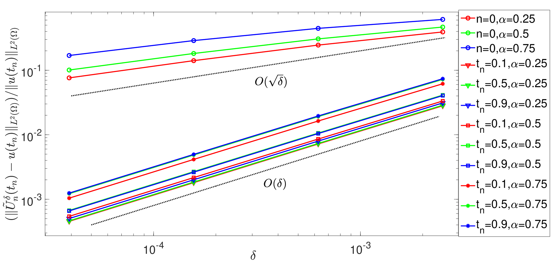
Refer to caption
Figure 2: Plot of ‖u⁡(tn)−U~nδ​(tn)‖L2​(Ω)/‖u⁡(tn)‖L2​(Ω)\|u(t_{n})-\tilde{U}_{n}^{\delta}(t_{n})\|_{L^{2}(\Omega)}/\|u(t_{n})\|_{L^{2}(\Omega)} with h=δh=\sqrt{\delta}, τ=δ\tau=\delta
and γ=δ\gamma=\sqrt{\delta} for tn=0t_{n}=0; and h=δh=\sqrt{\delta}, τ=δ\tau=\delta, γ=δ\gamma=\delta for tn>0t_{n}>0.

Example (b): Nonsmooth initial data.

Now we test numerical experiments with a step initial condition:

u0(x)={0,    0≤x≤12,1,12<x<1.u_{0}(x)=\left\{\eqalign{0,\,\,\,\,0\leq x\leq\frac{1}{2},\\ 1,\,\,\,\,\frac{1}{2}<x<1.}\right.

Since u0u_{0} is discontinuous and piecewise smooth, it is easy to see that u0∈H12−ϵ​(Ω)u_{0}\in H^{\frac{1}{2}-\epsilon}(\Omega) for any ϵ∈(0,12]\epsilon\in(0,\frac{1}{2}].

According to Theorem 3.2, we have the error estimate of the semidiscrete solution at t=0t=0:

‖u~hδ​(t)−u⁡(t)‖L2​(Ω)≤c⁡(γq/2+h2​ℓh1−q/2​γ−(2−q/2)+δ​γ−1),with​u0∈H˙q​(Ω).\hskip-43.36243pt\|\tilde{u}^{\delta}_{h}(t)-u(t)\|_{L^{2}(\Omega)}\leq c\big(\gamma^{q/2}+h^{2}\ell_{h}^{1-q/2}\gamma^{-(2-q/2)}+\delta\gamma^{-1}\big),\quad\mbox{with}~~u_{0}\in\dot{H}^{q}(\Omega).

This implies that the convergence rate may deteriorate when the initial data gets worse. This is fully supported by empirical results showed in Table 1, where we present the L2L^{2}-error of the semidiscrete solution at t=0t=0. In the computation, we let h=O⁡(δ45)h=O(\delta^{\frac{4}{5}}) and γ=O⁡(δ45)\gamma=O(\delta^{\frac{4}{5}}) in order to balance to noise level, regularization parameter and the discretization error. Then the empirical convergence rate is O⁡(δ15)O(\delta^{\frac{1}{5}}), which is consistent with the theoretical results.

Meanwhile, for a fixed t>0t>0, we have the error estimate (cf. Theorem 3.2)

‖u~hδ​(t)−u⁡(t)‖L2​(Ω)≤c⁡(γ​tq​α/2+γ−(1−q/2)​h2​ℓh1−q/2+δ)​t−α.\|\tilde{u}^{\delta}_{h}(t)-u(t)\|_{L^{2}(\Omega)}\leq c\big(\gamma\,t^{q\alpha/2}+\gamma^{-(1-q/2)}h^{2}\ell_{h}^{1-q/2}+\delta\big)t^{-\alpha}.

This implies the almost optimal scaling h=O⁡(δ78)h=O(\delta^{\frac{7}{8}}) and γ=O⁡(δ)\gamma=O(\delta), and the resulting optimal convergence rate O⁡(δ)O(\delta). This is supported by the numerical results shown in Table 2.

For the numerical reconstruction by the fully discrete scheme (4.9), we recall the result in Remark 4.1. To compute U~0δ\tilde{U}^{\delta}_{0}, we let γ=O⁡(δ45)\gamma=O(\delta^{\frac{4}{5}}), h=O⁡(δ45)h=O(\delta^{\frac{4}{5}}) and τ=O⁡(δ85)\tau=O(\delta^{\frac{8}{5}}), for a given δ\delta. Then our theory indicates an convergence rate of O⁡(δ15)O(\delta^{\frac{1}{5}}), which agrees well with the numerical results in Table 3. On the other hand, to compute U~nδ\tilde{U}^{\delta}_{n} for a fixed tn>0t_{n}>0 and δ>0\delta>0, we let h=δ74h=\delta^{\frac{7}{4}}, τ=O⁡(δ78)\tau=O(\delta^{\frac{7}{8}}) and γ=O⁡(δ)\gamma=O(\delta). Then the empirical convergence rate is close to O⁡(δ)O(\delta), which fully supports our theoretical estimates in Table 4.

Table 1: Example (b): error of u~hδ​(0)\tilde{u}_{h}^{\delta}(0), with δ=1/M\delta=1/M, h=γ=δ45h=\gamma=\delta^{\frac{4}{5}}.
α\M\alpha\backslash M 40 80 160 320 Rate(δ\delta)
0.25 4.68e-1 4.07e-1 3.48e-1 2.95e-1 0.22(0.20)
0.5 5.07e-1 4.46e-1 3.84e-1 3.27e-1 0.21(0.20)
0.75 5.70e-1 5.18e-1 4.59e-1 3.98e-1 0.17(0.20)
Table 2: Example (b): error of u~hδ​(t)\tilde{u}_{h}^{\delta}(t) at different tt with δ=1/M\delta=1/M, h=δ78h=\delta^{\frac{7}{8}}, γ=δ/5\gamma=\delta/5.
α\alpha t\Mt\backslash M 40 80 160 320 Rate(δ\delta)
0.1 7.91e-3 4.34e-3 2.30e-3 1.20e-3 0.91(1.00)
0.5 0.5 3.51e-3 1.93e-3 1.02e-3 5.33e-4 0.91(1.00)
0.9 2.41e-3 1.33e-3 7.13e-4 3.73e-4 0.90(1.00)
Table 3: Example (b): error of U~0δ\tilde{U}_{0}^{\delta}, with δ=1/M\delta=1/M, h=γ=δ45h=\gamma=\delta^{\frac{4}{5}}, τ=δ85\tau=\delta^{\frac{8}{5}}.
α\M\alpha\backslash M 40 80 160 320 Rate(δ\delta)
0.25 4.70e-1 4.07e-1 3.48e-1 2.96e-1 0.22(0.20)
0.5 5.08e-1 4.47e-1 3.85e-1 3.28e-1 0.21(0.20)
0.75 5.70e-1 5.17e-1 4.59e-1 3.98e-1 0.17(0.20)
Table 4: Example(b): error of U~nδ\tilde{U}_{n}^{\delta}, with δ=1/M\delta=1/M, h=δ78h=\delta^{\frac{7}{8}}, τ=δ74\tau=\delta^{\frac{7}{4}}, and γ=δ/5\gamma=\delta/5.
α\alpha tn\Mt_{n}\backslash M 40 80 160 320 Rate(δ\delta)
0.1 6.76e-3 3.82e-3 2.06e-3 1.08e-3 0.88(1.00)
0.5 0.5 3.46e-3 1.90e-3 1.01e-3 5.24e-4 0.91(1.00)
0.9 2.55e-3 1.40e-3 7.47e-4 3.89e-4 0.90(1.00)

Example (c): 2D problem.

Now we consider a two-dimensional problem in a unit square domain Ω=(0,1)2\Omega=(0,1)^{2}. We choose the smooth initial condition

u0​(x,y)=x⁡(1−x)​y​(1−y)∈H˙2​(Ω),u_{0}(x,y)=x(1-x)y(1-y)\in\dot{H}^{2}(\Omega),

and zero source term f≡0f\equiv 0. In the computation, we divided Ω\Omega into regular right triangles with KK equal subintervals of length h=1/Kh=1/K on each side of the domain. Here, we apply the conjugate gradient method to numerically solve the discrete system, instead of the direct approach by the spectral decomposition in Example (a) and (b).

For t=0t=0, we let h=γ=δ=τh=\gamma=\sqrt{\delta}=\sqrt{\tau}, and we observe that the convergence rate is O⁡(δ)O(\sqrt{\delta}), see Table 5). Moreover, In Table 6, we test the convergence rate for t=T/2t=T/2. By letting h=γ=δ=τh=\sqrt{\gamma}=\sqrt{\delta}=\sqrt{\tau}, the experiments show that the convergence rate is O⁡(δ)O(\delta). All emperical results agree well with our theoretical finding in Theorem 4.1.

Table 5: Example(c): error of U~0δ\tilde{U}_{0}^{\delta}, with δ=1/M\delta=1/M, h=δh=\sqrt{\delta}, τ=δ\tau=\delta, and γ=δ\gamma=\sqrt{\delta}.
α\M\alpha\backslash M 800 1600 3200 6400 Rate(δ\delta)
0.25 1.27e-2 9.57e-3 6.61e-3 3.96e-3 0.56(0.50)
0.5 1.57e-2 1.27e-2 9.53e-3 6.57e-3 0.42(0.50)
0.75 2.28e-3 1.96e-3 1.57e-3 1.11e-3 0.34(0.50)
Table 6: Example(c): error of U~nδ\tilde{U}_{n}^{\delta}, with tn=T/2t_{n}=T/2, δ=1/M\delta=1/M, h=δh=\sqrt{\delta}, τ=δ\tau=\delta, and γ=δ\gamma=\delta.
α\M\alpha\backslash M 800 1600 3200 6400 Rate(δ\delta)
0.25 5.09e-5 2.59e-5 1.31e-5 6.59e-6 0.98(1.00)
0.5 6.00e-5 3.08e-5 1.56e-5 7.90e-6 0.98(1.00)
0.75 7.06e-5 3.71e-5 1.89e-5 9.55e-6 0.96(1.00)

Acknowledgements

This project is partially supported by a Hong Kong RGC grant (project no. 25300818).

References

References

  • [1] E. G. Bajlekova. Fractional Evolution Equations in Banach Spaces. PhD thesis, Eindhoven University of Technology, 2001.
  • [2] D. N. Hào, J. Liu, N. V. Duc, and N. V. Thang. Stability results for backward time-fractional parabolic equations. Inverse Problems, 35(12):125006, 25, 2019.
  • [3] B. Jin, R. Lazarov, V. Thomée, and Z. Zhou. On nonnegativity preservation in finite element methods for subdiffusion equations. Math. Comp., 86(307):2239–2260, 2017.
  • [4] B. Jin, R. Lazarov, and Z. Zhou. Error estimates for a semidiscrete finite element method for fractional order parabolic equations. SIAM J. Numer. Anal., 51(1):445–466, 2013.
  • [5] B. Jin, B. Li, and Z. Zhou. Correction of high-order BDF convolution quadrature for fractional evolution equations. SIAM J. Sci. Comput., 39(6):A3129–A3152, 2017.
  • [6] B. Jin, B. Li, and Z. Zhou. Subdiffusion with a time-dependent coefficient: analysis and numerical solution. Math. Comp., 88(319):2157–2186, 2019.
  • [7] B. Jin and W. Rundell. A tutorial on inverse problems for anomalous diffusion processes. Inverse Problems, 31(3):035003, 40, 2015.
  • [8] A. A. Kilbas, H. M. Srivastava, and J. J. Trujillo. Theory and Applications of Fractional Differential Equations. Elsevier Science B.V., Amsterdam, 2006.
  • [9] Z. Li, Y. Liu, and M. Yamamoto. Inverse problems of determining parameters of the fractional partial differential equations. In Handbook of fractional calculus with applications. Vol. 2, pages 431–442. De Gruyter, Berlin, 2019.
  • [10] Z. Li and M. Yamamoto. Inverse problems of determining coefficients of the fractional partial differential equations. In Handbook of fractional calculus with applications. Vol. 2, pages 443–464. De Gruyter, Berlin, 2019.
  • [11] J. J. Liu and M. Yamamoto. A backward problem for the time-fractional diffusion equation. Appl. Anal., 89(11):1769–1788, 2010.
  • [12] Y. Liu, Z. Li, and M. Yamamoto. Inverse problems of determining sources of the fractional partial differential equations. In Handbook of fractional calculus with applications. Vol. 2, pages 411–429. De Gruyter, Berlin, 2019.
  • [13] C. Lubich. Discretized fractional calculus. SIAM J. Math. Anal., 17(3):704–719, 1986.
  • [14] R. Metzler, J.-H. Jeon, A. G. Cherstvy, and E. Barkai. Anomalous diffusion models and their properties: non-stationarity, non-ergodicity, and ageing at the centenary of single particle tracking. Phys. Chem. Chem. Phys., 16:24128, 37 pp., 2014.
  • [15] R. Metzler and J. Klafter. The random walk’s guide to anomalous diffusion: a fractional dynamics approach. Phys. Rep., 339(1):1–77, 2000.
  • [16] K. Sakamoto and M. Yamamoto. Initial value/boundary value problems for fractional diffusion-wave equations and applications to some inverse problems. J. Math. Anal. Appl., 382(1):426–447, 2011.
  • [17] H. Seybold and R. Hilfer. Numerical algorithm for calculating the generalized Mittag-Leffler function. SIAM J. Numer. Anal., 47(1):69–88, 2008/09.
  • [18] T. Simon. Comparing Fréchet and positive stable laws. Electron. J. Probab., 19:no. 16, 25, 2014.
  • [19] V. Thomée. Galerkin Finite Element Methods for Parabolic Problems. Springer-Verlag, Berlin, 2nd edition, 2006.
  • [20] J.-G. Wang and T. Wei. An iterative method for backward time-fractional diffusion problem. Numer. Methods Partial Differential Equations, 30(6):2029–2041, 2014.
  • [21] L. Wang and J. Liu. Total variation regularization for a backward time-fractional diffusion problem. Inverse Problems, 29(11):115013, 22, 2013.
  • [22] T. Wei and J.-G. Wang. A modified quasi-boundary value method for the backward time-fractional diffusion problem. ESAIM Math. Model. Numer. Anal., 48(2):603–621, 2014.
  • [23] M. Yang and J. Liu. Solving a final value fractional diffusion problem by boundary condition regularization. Appl. Numer. Math., 66:45–58, 2013.