DynaMiTe: A Dynamic Local Motion Model with Temporal Constraints for Robust Real-Time Feature Matching

Patrick Ruhkamp Ruiqi Gong Nassir Navab Benjamin Busam p.ruhkamp@tum.de b.busam@tum.de Affiliation: Technische Universität München, Germany

Abstract

Feature based visual odometry and SLAM methods require accurate and fast correspondence matching between consecutive image frames for precise camera pose estimation in real-time. Current feature matching pipelines either rely solely on the descriptive capabilities of the feature extractor or need computationally complex optimization schemes. We present the lightweight pipeline DynaMiTe, which is agnostic to the descriptor input and leverages spatial-temporal cues with efficient statistical measures. The theoretical backbone of the method lies within a probabilistic formulation of feature matching and the respective study of physically motivated constraints. A dynamically adaptable local motion model encapsulates groups of features in an efficient data structure. Temporal constraints transfer information of the local motion model across time, thus additionally reducing the search space complexity for matching. DynaMiTe achieves superior results both in terms of matching accuracy and camera pose estimation with high frame rates, outperforming state-of-the-art matching methods while being computationally more efficient.

1 Introduction

Visual self-localization from consecutive video frames of a freely moving camera has a long history [1] and is one of the key challenges in 3D computer vision. SLAM methods have been applied in robotics and UAVs [2] and are a crucial element in augmented reality pipelines [3] as well as medical applications [4]. Besides well known methods based on direct image alignment [3, 5, 6, 7], different sparse feature based methods are also well studied [8, 9, 10, 11].

Refer to caption — Figure 1: Comparison of feature matching for consecutive image frames on a challenging low-textured object of the TUM RGB-D dataset [12]. Features in frame $I_{i}$ in yellow; $I_{j}$ in green; Matches as blue lines. SIFT [13] is texture-sensitive. ORB [14] (2000 extractions) is efficient but unstable. GMS [15] produces noisy, wrong matches in uniform regions while our method runs the fastest with minimal incorrect matches.

Direct methods incorporate the image information directly from pixel intensities, which can be error-prone due to illumination changes, moving objects or shutter effects [5]. However, a dense image alignment can help with dense reconstructions of the scene [16]. Feature based methods rely on distinctive feature points extracted from the image input, which can account for illumination changes while reducing the computational complexity. Due to their sparseness, they are more suitable for SLAM methods with loop closures and bundle adjustment; however reconstructions are not dense [9].

The first step in feature based visual odometry and SLAM systems is to detect and to match keypoints between consecutive frames. Quality and robustness of this step is vital for camera pose estimation and all subsequent computations in the pipeline. Errors in pose estimation are usually treated in a second stage by pose optimization with local and global bundle adjustment or graph based optimization schemes [17, 18].

Motivation. Natura non facit saltus.¹¹ 1 Latin for ”nature does not make jumps”. This principle of natural philosophy was a crucial element in the formulation of infinitesimal calculus and classical mechanics [19]. Consequently, as

x\left(t+\Delta t\right)\approx x\left(t\right)+v_{0}\Delta t+\frac{1}{2}\,a\,\left(\Delta t\right)^{2},

(1)

we assume smooth motion of an object in space, which is also true for its projection $P\left(x\right)$ onto a camera image. Knowledge of the motion at time $t$ thus helps to approximate the projected location $P\left(x+\Delta t\right)$ in the next frame.

Given a video sequence, extracted feature points around descriptive parts of the image (e.g. some object in the scene) are grouped into local feature groups by our novel clustering algorithm. The spatial 2D displacement of corresponding groups is then propagated from previous frames by a motion proxy to constrain the search space for new feature matches. Since close features likely belong to the same scene structure, their motion is similar and inter-frame matches between corresponding groups can reinforce each other. This is justified by statistical measures based on a binomial distribution detailed in section 3.2. It follows that for a certain number of $n$ features in a group, a minimum number of $N$ matches between the groups is needed to confirm a true positive match (cf. Fig. 2).

Contributions and Outline. DynaMiTe combines two complementary elements of spatially coherent motion and temporarily smooth inter-frame displacements - analogous to its eponym - in its joint formulation for feature matching between consecutive image frames. To this end, DynaMiTe contributes:

1.

A dynamic local motion model encapsulating the differentiable spatial motion prior with temporal coherency constraints through frame-to-frame information passing.
2.

A statistical quality criteria to determine noise-free feature correspondences.
3.

An efficient clustering scheme through a light data structure to form groups of close-by feature points.
4.

An efficient and robust feature matching pipeline for camera pose estimation in image sequences that significantly improves the state-of-the-art evaluated on the three datasets KITTI [20], TUM RGB-D [12], and TILDE webcam [21].

To the best of our knowledge, DynaMiTe is the first method that uses a generic data structure to form clusters of feature points and combines spatial and temporal constraints for feature matching, formulated in a unified probabilistic model. We motivate our method by analyzing the shortcomings of similar approaches in Sec. 3. We then give an overview of the general procedure of DynaMiTe, introduce our proposed dynamic local motion model (Sec. 3.1), extend the probabilistic model of reinforcing support matches between groups of features (Sec. 3.2, 3.3), and deduce robust statistics from it (Sec. 3.4). In the experiments we show matching quality, robustness and repeatability on different datasets for DynaMiTe as well as runtime performance, outperforming SOTA even in challenging scenes.

2 Related Work

Feature based visual odometry methods have shown to achieve the tight real-time constraints to compute accurate camera poses and sparse 3D maps of the scene [8], even for long sequences [9]. Accurate feature matching has immediate effect on the subsequent tasks of pose estimation and map generation [22, 23, 24, 25, 26, 27]. Pose interpolation [28, 29] and filtering [30] techniques can be utilized to circumvent the real-time constraint for camera pose estimation from video sequences to some extent. To improve feature matching capabilities, multiple feature detectors and descriptors have been developed [13], also specifically targeting real-time applications [14]. One major area of research focuses on the development of robust descriptors which are less variant and more distinctive, thus enabling better matching performance [31]. Different descriptors [32, 33] and learning based pipelines [34, 35, 36, 37] enable a variety of vision applications [38, 39, 21, 40]. Some scholars design descriptor and detector together [40, 41, 42, 43, 44], or additionally learn the matching task [45] and also including semantic information [46]. Chli and Davison [47] propose to actively search for features by propagating information from the previous frame. Targeting specifically wide baseline, Yu et al. [48] proposed an efficient end-to-end pipeline for learning to find correspondences.

Differentiating between true correspondences and mismatches still remains as primary difficulty. Methods like the ratio test [13] improve feature matching quality by comparing the best and second best potential feature match. Cross check is an alternative to the ratio test, where the nearest neighbor matches are checked for consistency. Statistical approaches such as RANSAC [49] and its modifications [50, 51] are effective to remove outliers but may increase runtime due to their iterative execution, especially for large inputs. FLANN [52] finds approximate nearest neighbors in large datasets and can improve computation times.

By grouping joint motion pairs [53] different methods have been proposed in order to distinguish between true and false matches [54, 55]. Despite showing compelling results, their elaborate formulations result in complex and costly constraints. Other methods assume similar motion smoothness by matching patches between images [56, 57], or learn to match patches [58]. Sparse [59] and dense [60] optical flow algorithms [61] also assume neighboring points in 3D to move coherently.

Bian et al. [15] (GMS) were the first to formulate the idea of motion smoothness in space within a probabilistic model utilizing a predefined fixed pixel grid. Without GPU acceleration, their method is limited by its initial brute force matching to find potential candidates, many of which are being discarded as mismatches afterwards. Ma et al. [62] transfer the idea of close-by feature point matching directly to the Euclidean distance within consecutive frames. This approximation does not hold true in general and fails in practice for forward/backward translations, where the depth dependent projection scales non-uniformly. Also [63] employ locality information to filter match outliers and Zheng et al. [64] compute cluster centers from fixed grid patches to compare between frames. Wrong matches in the grid cells, however, shift the cluster center and the method requires initial brute force matching.

We also focus on improving matching quality by using close-by features for reinforcement, but propose a different clustering scheme, together with an improved probabilistic model for noise-free robust feature matches in video sequences. Unlike matching patches, we match single features where features around some landmark support each other.

3 Methodology

Problem Statement. Recent feature matching approaches [15, 64] for wide-baseline scenarios have introduced a simple probabilistic model to distinguish between correct matches and mismatches, where additional matches of proximate features reinforce each other. They are limited by analyzing those matches on regular grids or require expensive clustering algorithms. In the former scenario [15], high quantities of uniformly distributed feature points across the entire image are matched, and supporting matches within a regular grid are analyzed. A high number of feature points and uniform sampling lead to pairs of many keypoints with poor descriptor quality, resulting in noisy matches and a heavy computation. Proposed clustering algorithms as in [64] are very restrictive and show large variation based on their input, caused by unstable feature point detection between frames. The tight realtime constraint is problematic in both cases, as extracting and matching around 1E5 keypoints [15] is solely possible with GPU acceleration. Expensive clustering algorithms [64] aggravate the issue.

DynaMiTe. We take inspiration of supporting neighbouring matches [15] and extend the approach with our dynamic local clustering method to form groups of close-by feature points around descriptive landmarks.

After feature computation, our proposed method encapsulates the spatial group displacement by the cluster representative. The spatial cluster information is passed throughout the sequence in the temporal domain as motion proxy, resulting in a dynamic local motion model. Assuming mainly static scenes and smooth camera motion, only features of clusters within a certain search space around the cluster center in the previous frame need to be considered for matching. Hence, the group motion is used as prior to restrict the search space for potential matches, which are finally evaluated with our improved and robust probabilistic model. Algorithm 1 gives a general overview of our proposed pipeline, which is schematically detailed in Fig. 3.

forall Frame $I_{t}$ in video do 1

Extract feature points; 2

Establish feature groups (FG); 3

Calculate intersection of old and new FGs; 4

Match intersected FGs; 5

Compute match score and retrieve inlier; 6

Establish new FGs; 7

Pass FG information to next frame

I_{t+1}

; 8

Algorithm 1 DynaMiTe Pipeline for Feature Matching

We detail the foundation on how to establish a statistical measure for feature matching between patches with a matching score, and improve the base model with bi-directional matching to filter low confidence matches. Additionally, we extend the model with a locally adaptive clustering approach and adapt the underlying statistics for the probabilistic model. We show that the final probabilistic measure for feature matching only depends on the number of neighbouring feature points within a group and the number of supporting matches.

3.1 Dynamic Local Motion Model

We propose a fast and dynamic feature clustering approach by exploiting the nature of many feature detection operators to form clusters around descriptive landmarks in the scene. For this, Union-Find Disjoint Sets (UFDS) [65] is utilized for efficient grouping of close-by feature points. The data structure models groups in DynaMiTe as collection of disjoint sets.

UFDS is essentially a forest of multi-way trees, where each tree represents a disjoint subset of elements. A forest of trees can be implemented as an array $p$ of size $N$ items. $p[i]$ records the index of the parent of item $i$ . If $p[i]=i$ , then item $i$ is the root of this tree and also the representative item of the subset that contains item $i$ (cf. Fig. 4).

This allows to determine which set an item belongs to, check if two items belong to the same set, and merge two disjoint sets into one in nearly constant time (e.g. $O(1)$ ). In our 2 dimensional implementation, items are feature points and sets are groups. The efficiency of this operation is crucial as identifying the group of keypoints is a frequent operation and the correctness of every match is examined by the correlation between two groups.

Our 2D UFDS data structure considers the maximum size of a cluster in pixels as well as the min. and max. amount of features per group. This is justified by the probabilistic model derived hereafter (cf. 3.2). The analytic matching probabilities give the interval $[5,35]$ as a quality criterion for our group sizes which we also use in all our experiments. Cluster centers are initialized at random over the set of all extracted feature points. Algorithm details can be found in the suppl. material.

3.2 Probabilistic Model

Similar to [15] we assume that features within a close vicinity will match with a high probability to the same area in another image from a different viewpoint, matches of close-by features can reinforce each other. After feature points have been grouped with our proposed clustering algorithm, we analyze all enclosed features per intersecting groups between video frames. The rate of feature matches between patches compared to the number of enclosed keypoints gives a measure of certainty for the match. We can derive a probabilistic model by examining the matching events between correlated and uncorrelated image patches and deduce a binomial distribution which is only dependent on the number of enclosed keypoints in the patch. More specifically, we can define a threshold for a true positive match as the minimum amount of supporting feature matches between two groups relative to their enclosed keypoints.

Figure 1 illustrates the possible matching events (see Table 1 for notation). In case of observing corresponding patches $A,B$ (green case $T$ ) in two images $I_{i}$ and $I_{j}$ , we can observe a feature (green star) in patch $A$ that has its nearest neighbor (NN) in descriptor space in patch $B$ ( $f_{A}^{B}$ ). This feature can either be correctly matched ( $f_{A}$ ), or mismatched with some other feature in $B$ while its true NN lies still in $B$ ( $\overline{f_{A}},f_{A}^{B}$ ). We observe that those mismatches ( $\overline{f_{A}},f_{A}^{B}$ ) still contribute as ”noisy” support match between the patches. Similar observations can also be made for the false case $F$ , in which we analyze uncorrelated patches (e.g. patch $A^{\prime}$ and $B^{\prime}$ are not identical regions in the scene), where the feature is mismatched to its NN in $B^{\prime}$ ( $\overline{f_{A^{\prime}}},f_{A^{\prime}}^{B^{\prime}}$ ). By analyzing the matching events, it becomes apparent that there is a high probability of finding multiple matches between correlated patches which support each other.

Mathematical Justification. Let $f$ be one of $n$ features in $A$ , which we denote to correctly match to some feature out of $N$ features in $B$ as $f_{A}$ with $p(f_{A})=t$ . In case that feature $f$ matches wrongly (i.e. $\overline{f_{A}}$ ), its NN can be any of the other $N$ features in B. Thus, we can write

p\left(f_{A}^{B}\mid\overline{f_{A}}\right)=\frac{n}{N}.

(2)

For correlated patches (case $T$ ), we denote the probability that a feature in $A$ has its NN in $B$ by $p_{t}=p\left(f_{A}^{B}\mid T\right)$ . Examining the possible cases for $p_{t}$ as depicted in Fig. 1, this consists of a correct match $p\left(f_{A}\mid T\right)$ , or a mismatch while the NN is still in patch $B$ $p\left(\overline{f_{A}},f_{A}^{B}\mid T\right)$ . Therefore we can write:

\begin{split}p_{t}=p\left(f_{A}^{B}\mid T\right)&=p\left(f_{A}\mid T\right)+p\left(\overline{f_{A}},f_{A}^{B}\mid T\right)\\ &=p\left(f_{A}\mid T\right)+p\left(\overline{f_{A}}\mid T\right)\cdot p\left(f_{A}^{B}\mid\overline{f_{A}},T\right).\end{split}

(3)

With the assumption of independence for single feature matches, we are independent of $T$ . Using Baye’s rule, the notation from Table 1 and with Eq. 2, we get:

\begin{split}p_{t}&=p\left(f_{A}\right)+p\left(\overline{f_{A}}\right)\cdot p\left(f_{A}^{B}\mid\overline{f_{A}}\right)=t+\left(1-t\right)\cdot\dfrac{n}{N}.\end{split}

(4)

We assume that each group can be treated equally and that groups have similar numbers of features $N$ . Analogously for uncorrelated patches $A^{\prime}$ and $B^{\prime}$ (case $F$ ) we can derive:

\begin{split}p_{f}=p\left(f_{A^{\prime}}^{B^{\prime}}\mid F\right)&=p\left(\overline{f_{A^{\prime}}},f_{A^{\prime}}^{B^{\prime}}\mid F\right)=p\left(\overline{f_{A^{\prime}}}\mid F\right)\cdot p\left(f_{A^{\prime}}^{B^{\prime}}\mid\overline{f_{A^{\prime}}},F\right)\\ &=p\left(\overline{f_{A^{\prime}}}\right)\cdot p\left(f_{A^{\prime}}^{B^{\prime}}\mid\overline{f_{A^{\prime}}}\right)=\left(1-t\right)\cdot\dfrac{n}{N}.\end{split}

(5)

3.3 False Positive Reduction

Assuming some feature matches correctly or incorrectly with the same chances, i.e. $t=0.5$ , and with $n<<N$ , we get a wide separation between $p_{t}$ and $p_{f}$ (see Eqs. (4) and (5)). However, this is partly due to including noisy false positive matches, which is not desirable (compare noise for GMS in Fig. 1). To reduce noisy false positive matches (e.g. event ( $\overline{f_{A}},f_{A}^{B}$ ) in Fig. 1), we introduce a consistency check via bidirectional matching (compare Fig. 6). However, bidirectional matching has an influence on the terms in Eq. 4. Details on the derivation below are given in the suppl. material.

True Matches. Given correct patch associations $T$ , cross check $cc$ helps to reduce noisy matches. Let, similar to Eq. (3), the probability of a feature in $A$ having its NN in $B$ under cross check be $p_{t}^{cc}=p\left(f_{A}^{B}\mid T,cc\right)$ , then it holds:

\begin{split}p_{t}^{cc}&=p\left(f_{A}^{B}\mid T,cc\right)\\ &=\left(p\left(f_{A}\mid T\right)+p\left(\overline{f_{A}},f_{A}^{B}\mid T\right)\right)\cdot\left(p\left(f_{B}\mid T\right)+p\left(\overline{f_{B}},f_{B}^{A}\mid T\right)\right).\end{split}

(6)

As before (see Eqs. (3) and (4)), with $m$ and $M$ being the equivalent for $n$ and $N$ and by substitution after the binomial expansion, we can reduce this to:

p_{t}^{cc}=t^{2}+2\cdot t\cdot\left(1-t\right)\dfrac{n}{N}+\left(1-t\right)^{2}\dfrac{n}{N}\cdot\dfrac{m}{M}

(7)

False Matches. In analogy for uncorrelated patches it holds:

\begin{split}p_{f}^{cc}&=p\left(\overline{f_{A^{\prime}}},f_{A^{\prime}}^{B^{\prime}}\mid F\right)\cdot p\left(\overline{f_{B^{\prime}}},f_{B^{\prime}}^{A}\mid F\right)=\left(1-t\right)^{2}\dfrac{n}{N}\cdot\dfrac{m}{M}\end{split}

(8)

3.4 Robust Statistics

Naive bidirectional matching between all features is expensive, especially for the extraction of a large quantity (around $1E5$ ) of uniformly distributed features in the image as in [15]. Additionally, the fraction of $n/N$ becomes small, as a few features $n$ in a patch are compared against all features $N$ of the entire image, which would reduce the separation between $p_{t}$ and $p_{f}$ .

As our proposed model embeds spatial and temporal information and can serve as a motion proxy of the displacement of encapsulated feature points, the potential feature matches are restricted to the intersecting clusters within a certain search space. Thus, not only the computational bottleneck is reduced, but also $N$ decreases significantly. With the assumption of small inter-frame motion, the number of features in $A$ and $B$ are similar ( $n\approx N$ ) and the fraction in Eq. 7 and Eq. 8 reaches $1$ , yielding again a wide separation between $p_{t}$ and $p_{f}$ . Additionally, we suppose $p\left(f_{A}\right)=t$ to be larger than $0.5$ which increases the wide seperation.

Matching Quality Criterion. Matching of an individual feature is generally independent of other features. Thus, we can use the derivations from above similar to [15] to formulate a binomial distribution which describes the probability of finding additional support matches between correlated or uncorrelated groups for some feature match $m_{i}^{j}$ . Our matching quality criterion $Q_{i}$ is dependent of the number on feature points $n$ in a patch:

Q_{i}=\begin{cases}B(n,p_{t}^{cc}),&\text{if}\quad m_{i}^{j}\quad\text{is true}\\ B(n,p_{f}^{cc}),&\text{if}\quad m_{i}^{j}\quad\text{is false}\end{cases}

(9)

\mu_{t}=np_{t}^{cc},\sigma_{t}=\sqrt{np_{t}^{cc}(1-p_{t}^{cc})}\quad\text{if}\quad m_{i}^{j}\quad\text{is true}

(10)

\mu_{f}=np_{f}^{cc},\sigma_{f}=\sqrt{np_{f}^{cc}(1-p_{f}^{cc})}\quad\text{if}\quad m_{i}^{j}\quad\text{is false}.

(11)

From a statistical viewpoint, this allows us to formulate a reliable criterion to decide whether or not two groups are correlated and therefore enclose true matches. The objective is to identify a wide separation between true and false cases. Such a division is given, if one event is at least $k=2$ standard deviations $\sigma_{f}$ apart from the mean $\mu_{f}$ (cf. Fig. 7). This reduces the probabilities to a simple threshold $\tau$ .

As $\mu_{f}$ is small (see Eqs. (8) and (11)) and $\sigma_{f}$ is mainly dependent on the number of features $n$ (for $\sigma_{f}$ in Eq. (11), the $p_{f}^{cc}(1-p_{f}^{cc})$ becomes very small), we can write the support threshold as:

\tau=\mu_{f}+k\sigma_{f}\approx k\sqrt{n}.

(12)

For a given number of features $n$ in a group, we can compute $\tau$ and compare with the number of other supporting matches between the patches. Is the number of supporting matches higher than $\tau$ , the patches are correlated and the feature matches between them identified as correct.

4 Experimental Evaluation

We quantitatively compare our method against a number of proposed classical matching approaches GMS [15], SIFT [13], SURF [32], ORB [14], BD [66], BF [55], GAIM [67], USC [68] as well as learning based methods DM [69] and LIFT [40]. We compare on different datasets with small (TUM [12]) and large (Kitti [20]) baselines as well as scenes with little texture (Cabinet [12]).

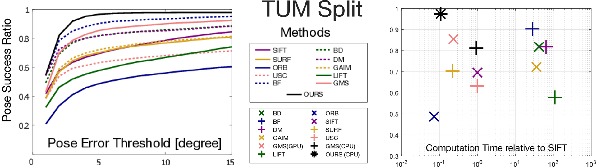
Evaluation aspects are based on matching accuracy, robustness and runtime. To quantify matching accuracy, we evaluate the accuracy of pose estimation from matched features and follow the evaluation protocol of Bian et al. [15] and use their results for comparison on the TUM split. Pose success ratio is reported as a measure of correctly recovered poses under a certain error threshold. The pose is recovered by the estimated essential matrix from feature matches with a RANSAC scheme. The improved results over the SOTA confirm that our proposed spatial-temporal probabilistic model is beneficial in a wide range of textured scenes and different baselines. We observe less convincing results in scenes with limited texture (”Cabinet”, see Fig. 1 as example) and explain this as limited ability to form feature groups for such scenes. We justify our assumption by analyzing the average inlier ratio of feature matches of the RANSAC scheme during pose estimation. Matching repeatability is analyzed as reprojection error of feature matches in static scenes. Additional qualitative results are provided as well as an ablation study by disabling parts of the method, thus examining the limitations of our approach.

All experiments are conducted on an Intel Core i7 CPU. We use the publicly available ORB implementation of OpenCV [70]. For more details on the maximum number of extracted feature points and parametrization of UFDS please refer to the suppl. material.

Matching Accuracy. Evidently, DynaMiTe outperforms other methods in textured scenarios [12], as the full potential of our joint formulation of spatial and temporal constraints can unfold (Fig. 8 [Left]).

Runtime. We have tested runtime performance on Kitti [20] and TUM [12]. Our method outperforms SIFT and optical flow (OF) [59] as baselines and even GMS [15] with GPU acceleration (compare GMS-GPU [15] in Tab. 2).

	OF [59]	SIFT [13]	GMS [15]	GMS-GPU	Ours
Kitti	14	18	3	12	44
TUM	48*	22	4	14	63

Table 2: Runtime in frames per second (fps). For OF* we report fastest observed fps, as it varies extensively depending on the scene structure and camera displacement.

Runtime vs. Accuracy. For better comparison we evaluate accuracy against runtime (cf. Fig. 8 [Right]). DynaMiTe consistently outperforms other methods in terms of runtime vs. success ratio.

Low-Texture scene. For the low-texture scene ”Cabinet”, tracking a large number of group associations throughout the entire sequence is challenging. Only a small number of groups with enough feature points cluster around well defined landmarks. DynaMiTe still performs on par with other methods, which also have difficulties in this scenario and ranks top in terms of runtime vs. accuracy (compare Fig. 9).

Inlier ratio. To analyze the inferior results on ”Cabinet”, we add the inliers of RANSAC during camera pose estimation in Tab. 3. The results reflect our findings, as both pose success and inlier ratio for the textured scenes are superior with DynaMiTe, whereas the Cabinet scene with little structure is challenging.

	OF [59]	SIFT [13]	SIFT*	GMS [15]	Ours
TUM Split	0.58	0.16	0.54	0.18	0.32
Cabinet	0.50	0.20	0.61	0.24	0.22
Kitti	0.37	0.11	0.64	0.85	0.87

Table 3: Avg. inlier ratio of RANSAC scheme for pose recovery relative to matches. SIFT* includes additional filtering of matches with ratio test.

Matching repeatability. In Tab. 4 the average match reprojection error for different static scenes from the TILDE webcam dataset [21] are summarized. For a perfect match, the norm would be assumed to be $0$ , as the scene and the camera remain static throughout the video. This metric can be interpreted as a measure for matching repeatability and the accuracy of the matching scheme as high errors indicate wrong and noisy matches and the inability to robustly handle repetitive patterns. DynaMiTe considerably outperforms SIFT as baseline and reports superior results compared to GMS.

	Chamonix	Courbevone	Frankfurt	Mexico	Panorama	St. Louis
SIFT [13]	196.03	184.70	298.17	175.24	592.85	215.27
GMS [15]	3.48	4.34	7.21	9.47	142.10	8.33
Ours	1.92	2.47	9.45	6.75	2.80	3.97

Table 4: Feature matching repeatability test on TILDE dataset [21] as average

L_{2}

reprojection error in pixels.

As an additional measure to the evaluation in Tab. 4, the error relative to the number of extracted feature points for GMS and our method is analyzed. We calculate the average $L_{2}$ error normalized per $1000$ features for each sequence and report the average of those as $2.92$ for GMS and $\bf{0.67}$ for DynaMiTe, which underlines the favourable efficiency and accuracy of our approach.

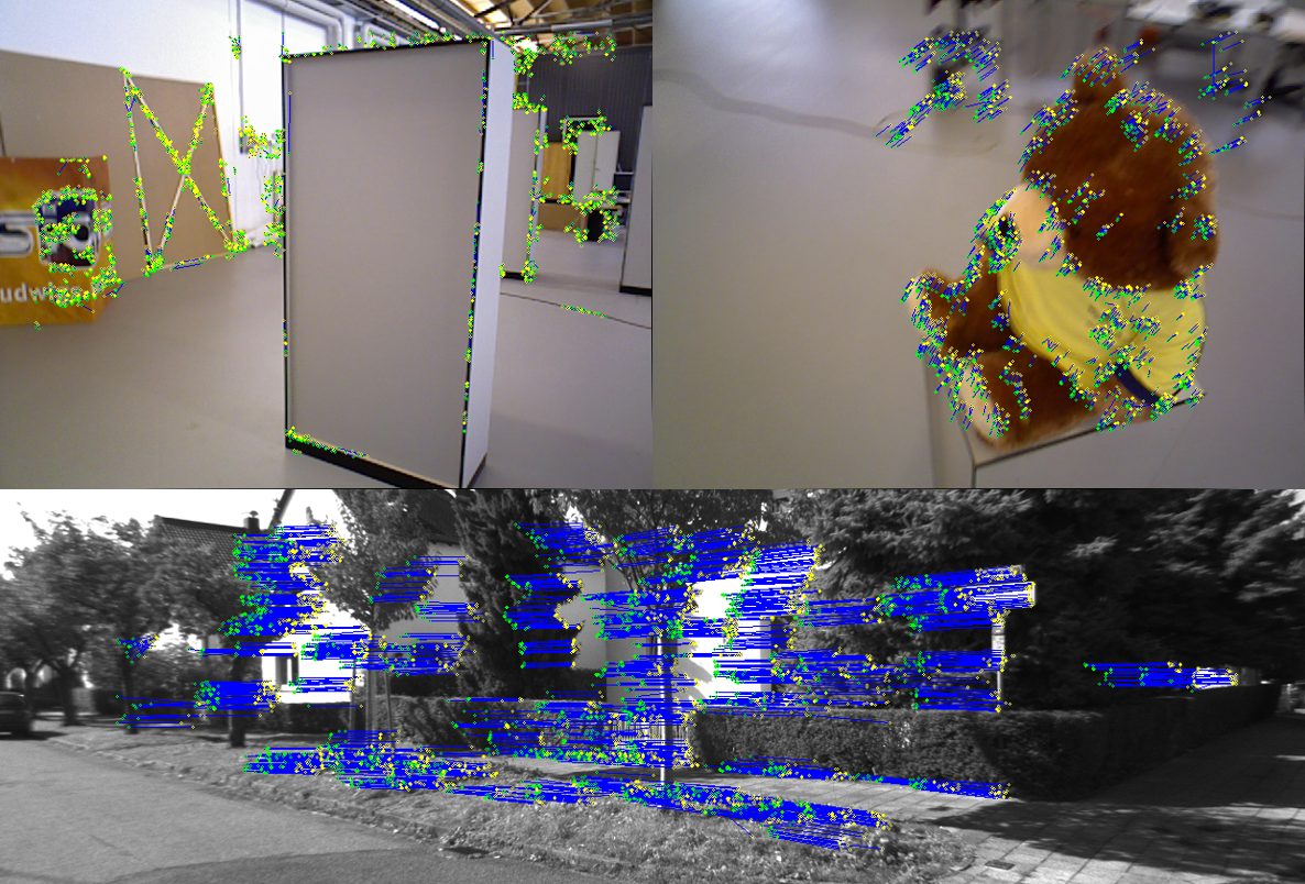
Qualitative Robustness Evaluation. We present additional qualitative results on matching robustness in different scenes. Our method filters out noisy, not meaningful matches of the texture-less background. Furthermore, our proposed cluster grouping and spatial-temporal formulation robustly tracks reliable features around landmarks with high image information (e.g. edges and corners of the cabinet, see Fig. 1 and 10 [Left]). DynaMiTe can also handle repetitive patterns in the Kitti sequence, such as the windows on the white building, due to its local clustering algorithm, whereas regular grids such as in GMS fail (see Fig. 10 [Right]).

Ablation Study. The experiments above show applicability on small and wide baseline scenarios (TUM/Kitti). Here, we specifically force the algorithm to only keep matches between groups which have been matched throughout the sequence of $10$ consecutive frames and not to establish new group associations between frames. Due to large inter-frame forward motion, only a few groups in the center of the image are reliably visible throughout all frames. While our assumptions hold true for consecutive frames, tracking the complete sequence from frame at time step $t$ to $t+10$ is problematic as our constraints are violated in this particular setting. Fig. 11 illustrates the limitations of our proposed method in this specific case. DynaMiTe can still be applied in scenarios with very large baselines, however at the cost of a relaxed constraint for inter-frame motion by increasing the search space for the temporal motion prior.

5 Discussion

The reported results clearly show the fundamental trade-off between the ability to correctly match feature points and comply with the runtime constraint for different matching methods. DynaMiTe reduces this limitation with its joint formulation, as it efficiently passes information throughout the sequence, encapsulated in the joint spatial-temporal model This enables very robust feature matching, as well as reduced noise in low-textured scenes, and high framerates without GPU acceleration. High-confidence noise-free feature matches are beneficial for camera pose estimation, which is what our method focuses on. The same holds true for reconstruction purposes, one of the various possible application scenarios for DynaMiTe. Generally, our proposed pipeline utilizes solely the information of the feature descriptor and its pixel location in the image, while being agnostic to the underlying descriptor itself. Our model achieves robust feature matching even in difficult scenarios and arbitrary inter-frame motion such as scaling and in-plane rotations, as we rely neither on regular grids nor restrictive clustering methods.

References

[1] Matthies, L., Szeliski, R., Kanade, T.: Incremental estimation of dense depth maps from image sequences. In: Computer Vision and Pattern Recognition, 1988. Proceedings CVPR’88., Computer Society Conference on, IEEE (1988) 366–374
[2] von Stumberg, L., Usenko, V., Engel, J., Stückler, J., Cremers, D.: From monocular slam to autonomous drone exploration. In: 2017 European Conference on Mobile Robots (ECMR), IEEE (2017) 1–8
[3] Engel, J., Koltun, V., Cremers, D.: Direct sparse odometry. IEEE Transactions on Pattern Analysis and Machine Intelligence 4(3) (2017) 611–625
[4] Busam, B., Ruhkamp, P., Virga, S., Lentes, B., Rackerseder, J., Navab, N., Hennersperger, C.: Markerless Inside-Out Tracking for 3D Ultrasound Compounding. In: Simulation, Image Processing, and Ultrasound Systems for Assisted Diagnosis and Navigation, Cham, Springer (2018) 56–64
[5] Engel, J., Sch, T., Cremers, D.: LSD-SLAM: Direct Monocular SLAM. In: European Conference on Computer Vision (ECCV), Cham, Springer (2014) 834–849
[6] Hanna, K.: Direct multi-resolution estimation of ego-motion and structure from motion. In: Visual Motion, 1991., Proceedings of the IEEE Workshop on, IEEE (1991) 156–162
[7] Newcombe, R.A., Izadi, S., Hilliges, O., Molyneaux, D., Kim, D., Davison, A.J., Kohi, P., Shotton, J., Hodges, S., Fitzgibbon, A.: KinectFusion: Real-time dense surface mapping and tracking. In: Mixed and augmented reality (ISMAR), 2011 10th IEEE international symposium on, IEEE (2011) 127–136
[8] Klein, G., Murray, D.: Parallel Tracking and Mapping for Small AR Workspaces. In: Mixed and Augmented Reality, 2007. ISMAR 2007. 6th IEEE and ACM International Symposium on. (2007) 225–234
[9] Mur-Artal, R., Tardos, J.D.: ORB-SLAM2: An Open-Source SLAM System for Monocular, Stereo, and RGB-D Cameras. IEEE Transactions on Robotics 33(5) (10 2017) 1255–1262
[10] Klein, G., Murray, D.W.: Full-3D Edge Tracking with a Particle Filter. In: BMVC. (2006) 1119–1128
[11] Davison, A.J., Reid, I.D., Molton, N.D., Stasse, O.: Monoslam: Real-time single camera slam. IEEE Transactions on Pattern Analysis & Machine Intelligence (2007) 1052–1067
[12] Sturm, J., Engelhard, N., Endres, F., Burgard, W., Cremers, D.: A benchmark for the evaluation of RGB-D SLAM systems. In: Intelligent Robots and Systems (IROS), 2012 IEEE/RSJ International Conference on, IEEE (2012) 573–580
[13] Lowe, D.G.: Distinctive Image Features from Scale-Invariant Keypoints. International Journal of Computer Vision 60(2) (2004) 91–110
[14] Rublee, E., Rabaud, V., Konolige, K., Bradski, G.: ORB: An efficient alternative to SIFT or SURF. In: Computer Vision (ICCV), 2011 IEEE international conference on. (11 2011) 2564–2571
[15] Bian, J., Lin, W.Y., Matsushita, Y., Yeung, S.K., Nguyen, T.D., Cheng, M.M.: GMS: Grid-Based Motion Statistics for Fast, Ultra-Robust Feature Correspondence. In: 2017 IEEE Conference on Computer Vision and Pattern Recognition (CVPR). (7 2017) 2828–2837
[16] Cremers, D.: Direct methods for 3d reconstruction and visual slam. In: 2017 Fifteenth IAPR International Conference on Machine Vision Applications (MVA), IEEE (2017) 34–38
[17] Kummerle, R., Grisetti, G., Strasdat, H., Konolige, K., Burgard, W.: G2o: A general framework for graph optimization. In: Robotics and Automation (ICRA), 2011 IEEE International Conference on, IEEE (2011) 3607–3613
[18] Strasdat, H., Davison, A.J., Montiel, J., Konolige, K.: Double window optimisation for constant time visual SLAM. In: Computer Vision (ICCV), 2011 IEEE International Conference on. (2011) 2352–2359
[19] Baumgarten, A.: Metaphysics: A Critical Translation with Kant’s Elucidations, Selected Notes, and Related Materials. A&C Black (2013)
[20] Geiger, A., Lenz, P., Stiller, C., Urtasun, R.: Vision meets robotics: The KITTI dataset. The International Journal of Robotics Research 32(11) (2013) 1231–1237
[21] Verdie, Y., Kwang Moo Yi, Fua, P., Lepetit, V.: TILDE: A Temporally Invariant Learned DEtector. In: Proceedings of the IEEE Conference on Computer Vision and Pattern Recognition. (6 2015) 5279–5288
[22] Nister, D.: An efficient solution to the five-point relative pose problem. IEEE Transactions on Pattern Analysis and Machine Intelligence 26(6) (6 2004) 756–770
[23] Hesch, J.A., Roumeliotis, S.I.: A Direct Least-Squares (DLS) method for PnP. In: 2011 International Conference on Computer Vision, IEEE (2011) 383–390
[24] Lepetit, V., Moreno-Noguer, F., Fua, P.: EPnP: An Accurate O(n) Solution to the PnP Problem. International Journal of Computer Vision 81(2) (2009) 155–166
[25] Penate-Sanchez, A., Andrade-Cetto, J., Moreno-Noguer, F.: Exhaustive Linearization for Robust Camera Pose and Focal Length Estimation. IEEE Transactions on Pattern Analysis and Machine Intelligence 35(10) (2013) 2387–2400
[26] Xiao-Shan Gao, Xiao-Rong Hou, Jianliang Tang, Hang-Fei Cheng: Complete solution classification for the perspective-three-point problem. IEEE Transactions on Pattern Analysis and Machine Intelligence 25(8) (2003) 930–943
[27] Fathian, K., Ramirez-Paredes, J.P., Doucette, E.A., Curtis, J.W., Gans, N.R.: Quaternion based camera pose estimation from matched feature points. arXiv preprint arXiv:1704.02672 (2017)
[28] Busam, B., Esposito, M., Frisch, B., Navab, N.: Quaternionic Upsampling: Hyperspherical Techniques for 6 DoF Pose Tracking. In: 2016 Fourth International Conference on 3D Vision (3DV), IEEE (10 2016) 629–638
[29] Shoemake, K.: Animating rotation with quaternion curves. In: Proceedings of the 12th annual conference on Computer graphics and interactive techniques - SIGGRAPH ’85, ACM Press (1985) 245–254
[30] Busam, B., Birdal, T., Navab, N.: Camera Pose Filtering with Local Regression Geodesics on the Riemannian Manifold of Dual Quaternions. In: Proceedings - 2017 IEEE International Conference on Computer Vision Workshops, ICCVW 2017. Volume 2018-Janua., IEEE (2018) 2436–2445
[31] Csurka, G., Humenberger, M.: From handcrafted to deep local invariant features. arXiv preprint arXiv:1807.10254 (7 2018)
[32] Bay, H., Ess, A., Tuytelaars, T., Van Gool, L.: Speeded-Up Robust Features (SURF). Computer Vision and Image Understanding 110(3) (2008) 346–359
[33] Morel, J.M., Yu, G.: ASIFT: A New Framework for Fully Affine Invariant Image Comparison. SIAM Journal on Imaging Sciences 2(2) (2009) 438–469
[34] Balntas, V., Riba, E., Ponsa, D., Mikolajczyk, K.: Learning local feature descriptors with triplets and shallow convolutional neural networks. In: BMVC. Volume 1. (2016) 3
[35] Tian, Y., Fan, B., Wu, F.: L2-net: Deep learning of discriminative patch descriptor in euclidean space. In: Proceedings of the IEEE Conference on Computer Vision and Pattern Recognition. (2017) 661–669
[36] Mishchuk, A., Mishkin, D., Radenovic, F., Matas, J.: Working hard to know your neighbor’s margins: Local descriptor learning loss. In: Advances in Neural Information Processing Systems. (2017) 4826–4837
[37] Tian, Y., Yu, X., Fan, B., Wu, F., Heijnen, H., Balntas, V.: Sosnet: Second order similarity regularization for local descriptor learning. In: Proceedings of the IEEE Conference on Computer Vision and Pattern Recognition. (2019) 11016–11025
[38] Choy, C.B., Gwak, J., Savarese, S., Chandraker, M.: Universal correspondence network. In: Advances in Neural Information Processing Systems. (2016) 2414–2422
[39] Simo-Serra, E., Trulls, E., Ferraz, L., Kokkinos, I., Fua, P., Moreno-Noguer, F.: Discriminative Learning of Deep Convolutional Feature Point Descriptors. In: 2015 IEEE International Conference on Computer Vision (ICCV), IEEE (2015) 118–126
[40] Yi, K.M., Trulls, E., Lepetit, V., Fua, P.: LIFT: Learned Invariant Feature Transform. European Conference on Computer Vision (2016) 467–483
[41] Ono, Y., Trulls, E., Fua, P., Yi, K.M.: Lf-net: learning local features from images. In: Advances in Neural Information Processing Systems. (2018) 6234–6244
[42] DeTone, D., Malisiewicz, T., Rabinovich, A.: SuperPoint: Self-Supervised Interest Point Detection and Description. CVPR Deep Learning for Visual SLAM Workshop (12 2017)
[43] Shen, X., Wang, C., Li, X., Yu, Z., Li, J., Wen, C., Cheng, M., He, Z.: Rf-net: An end-to-end image matching network based on receptive field. In: Proceedings of the IEEE Conference on Computer Vision and Pattern Recognition. (2019) 8132–8140
[44] Dusmanu, M., Rocco, I., Pajdla, T., Pollefeys, M., Sivic, J., Torii, A., Sattler, T.: D2-net: A trainable cnn for joint detection and description of local features. arXiv preprint arXiv:1905.03561 (2019)
[45] Sarlin, P.E., DeTone, D., Malisiewicz, T., Rabinovich, A.: Superglue: Learning feature matching with graph neural networks (2019)
[46] Ufer, N., Ommer, B.: Deep semantic feature matching. In: Proceedings of the IEEE Conference on Computer Vision and Pattern Recognition (CVPR). (2017)
[47] Chli, M., Davison, A.: Active matching. In: ECCV. (10 2008) 72–85
[48] Yi, K.M., Trulls, E., Ono, Y., Lepetit, V., Salzmann, M., Fua, P.: Learning to Find Good Correspondences. In: Proceedings of the 2018 IEEE/CVF Conference on Computer Vision and Pattern Recognition. (2018)
[49] Fischler, M.A., Bolles, R.C.: Random sample consensus: a paradigm for model fitting with applications to image analysis and automated cartography. Communications of the ACM 24(6) (6 1981) 381–395
[50] Chum, O., Matas, J.: Matching with PROSAC — Progressive Sample Consensus. In: Computer Vision and Pattern Recognition, 2005. CVPR 2005. IEEE Computer Society Conference on. Volume 1., IEEE (2005) 220–226
[51] Mintz, D., Meer, P., Rosenfeld, A.: Analysis of the least median of squares estimator for computer vision applications. In: Computer Vision and Pattern Recognition, 1992. Proceedings CVPR’92., 1992 IEEE Computer Society Conference on, IEEE Comput. Soc. Press (1992) 621–623
[52] Muja, M., Muja, M., Lowe, D.G.: Fast approximate nearest neighbors with automatic algorithm configuration. IN VISAPP INTERNATIONAL CONFERENCE ON COMPUTER VISION THEORY AND APPLICATIONS (2009) 331–340
[53] Yuille, A., Grzywacz, N., Norberto, M.: The Motion Coherence Theory. In: 1988 Second International Conference on Computer Vision, IEEE (1988) 344–353
[54] Lin, W.Y., Wang, F., Cheng, M.M., Yeung, S.K., Torr, P.H., Do, M.N., Lu, J.: CODE: Coherence Based Decision Boundaries for Feature Correspondence. IEEE Transactions on Pattern Analysis and Machine Intelligence 40(1) (2018) 34–47
[55] Lin, W.y.D., Cheng, M.m., Lu, J., Yang, H., Do, M.N., Torr, P.: Bilateral Functions for Global Motion Modeling. In: European Conference on Computer Vision. (2014) 341–356
[56] Barnes, C., Shechtman, E., Finkelstein, A., Goldman, D.B.: PatchMatch: A randomized correspondence algorithm for structural image editing. ACM Transactions on Graphics (ToG) 28(3) (2009) 24
[57] HaCohen, Y., Shechtman, E., Goldman, D.B., Lischinski, D.: Non-rigid dense correspondence with applications for image enhancement. In: ACM transactions on graphics (TOG), ACM (2011)
[58] Xufeng Han, Leung, T., Jia, Y., Sukthankar, R., Berg, A.C.: Matchnet: Unifying feature and metric learning for patch-based matching. In: 2015 IEEE Conference on Computer Vision and Pattern Recognition (CVPR). (June 2015) 3279–3286
[59] Lucas, B.D., Kanade, T.: An iterative image registration technique with an application to stereo vision. In: Proceedings of the 7th International Joint Conference on Artificial Intelligence - Volume 2. IJCAI’81, San Francisco, CA, USA, Morgan Kaufmann Publishers Inc. (1981) 674–679
[60] Farnebäck, G.: Two-Frame Motion Estimation Based on Polynomial Expansion. In: Image Analysis. Springer (2003) 363–370
[61] Horn, B.K., Schunck, B.G.: Determining optical flow. Artificial Intelligence 17(1-3) (1981) 185–203
[62] Ma, J., Zhao, J., Jiang, J., Zhou, H., Guo, X.: Locality Preserving Matching. International Journal of Computer Vision (2017) 1–20
[63] Wang, G., Chen, Y., Zheng, X.: Gaussian field consensus: A robust nonparametric matching method for outlier rejection. Pattern Recognition 74 (2018) 305–316
[64] Zheng, Z., Ma, Y., Zheng, H., Ju, J., Lin, M.: UGC: Real-time, Ultra-robust Feature Correspondence via Unilateral Grid-based Clustering. IEEE Access (2018)
[65] Galler, B.A., Fisher, M.J.: An Improved Equivalence Algorithm. Communications of the ACM 7(5) (1964) 301–303
[66] Lipman, Y., Yagev, S., Poranne, R., Jacobs, D.W., Basri, R.: Feature matching with bounded distortion. ACM Transactions on Graphics (TOG) 33(3) (2014) 26
[67] Collins, T., Mesejo, P., Bartoli, A.: An analysis of errors in graph-based keypoint matching and proposed solutions. In: European Conference on Computer Vision, Springer (2014) 138–153
[68] Raguram, R., Chum, O., Pollefeys, M., Matas, J., Frahm, J.M.: USAC: a universal framework for random sample consensus. IEEE Trans. Pattern Anal. Mach. Intell. 35(8) (2013) 2022–2038
[69] Weinzaepfel, P., Revaud, J., Harchaoui, Z., Schmid, C.: DeepFlow: Large displacement optical flow with deep matching. In: Proceedings of the IEEE International Conference on Computer Vision. (2013) 1385–1392
[70] Bradski, G.: The OpenCV Library. Dr. Dobb’s Journal of Software Tools (2000)

Appendix 0.A Details on 3.3 False Positive Reduction

Here, we detail the derivation of Eq. (6) from the main paper for better understandability.

True Matches. Let the probability of a feature in $A$ having its Nearest Neighbor in $B$ under cross check be $p_{t}^{cc}=p\left(f_{A}^{B}\mid T,cc\right)$ , then it holds:

	$\displaystyle p_{t}^{cc}$	$\displaystyle=p\left(f_{A}^{B}\mid T,cc\right)$
		$\displaystyle=\left(p\left(f_{A}\mid T\right)+p\left(\overline{f_{A}},f_{A}^{B}\mid T\right)\right)\cdot\left(p\left(f_{B}\mid T\right)+p\left(\overline{f_{B}},f_{B}^{A}\mid T\right)\right)$
		$\displaystyle=\left(p\left(f_{A}\mid T\right)+p\left(\overline{f_{A}}\mid T\right)\cdot p\left(f_{A}^{B}\mid\overline{f_{A}},T\right)\right)$
		$\displaystyle\qquad\qquad\qquad\qquad\cdot\left(p\left(f_{B}\mid T\right)+p\left(\overline{f_{B}}\mid T\right)\cdot p\left(f_{B}^{A}\mid\overline{f_{B}},T\right)\right)$

		as we are independent of $T$ and with $p\left(f_{A}^{B}\mid\overline{f_{A}}\right)=\frac{n}{N})$ ,
		where $m$ and $M$ are equivalent to $n$ and $N$ :

		$\displaystyle=\left(p\left(f_{A}\right)+p\left(\overline{f_{A}}\right)\cdot\dfrac{n}{N}\right)\cdot\left(p\left(f_{B}\right)+p\left(\overline{f_{B}}\right)\cdot\dfrac{m}{M}\right)$

		with $p\left(f_{A}\right)=p\left(f_{B}\right)=t$ :

		$\displaystyle=\left(t+\left(1-t\right)\cdot\dfrac{n}{N}\right)\cdot\left(t+\left(1-t\right)\cdot\dfrac{m}{M}\right)$

		after binomial expansion:

		$\displaystyle=t^{2}+2\cdot t\cdot\left(1-t\right)\dfrac{n}{N}+\left(1-t\right)^{2}\dfrac{n}{N}\cdot\dfrac{m}{M}$

False Matches. In analogy for uncorrelated patches:

	$\displaystyle p_{f}^{cc}$	$\displaystyle=p\left(\overline{f_{A^{\prime}}},f_{A^{\prime}}^{B^{\prime}}\mid F\right)\cdot p\left(\overline{f_{B^{\prime}}},f_{B^{\prime}}^{A^{\prime}}\mid F\right)$
		$\displaystyle=p\left(\overline{f_{A^{\prime}}}\mid F\right)\cdot p\left(\overline{f_{A^{\prime}}}\mid f_{A^{\prime}}^{B^{\prime}},F\right)\cdot p\left(\overline{f_{B^{\prime}}}\mid F\right)\cdot p\left(\overline{f_{B^{\prime}}}\mid f_{B^{\prime}}^{A^{\prime}},F\right)$
		$\displaystyle=p\left(\overline{f_{A^{\prime}}}\right)\cdot\dfrac{n}{N}\cdot p\left(\overline{f_{B^{\prime}}}\right)\cdot\dfrac{m}{M}$
		$\displaystyle=\left(1-t\right)^{2}\dfrac{n}{N}\cdot\dfrac{m}{M}$

Appendix 0.B Runtime Analysis

Our method achieves realtime performance on CPU for the full pipeline from feature extraction, matching and applying our spatial and temporal constraints, without any GPU acceleration. In Fig. 12 the runtime advantage of our method against GMS is clearly visible. GMS is by a factor of 4 slower with GPU acceleration and for CPU-only even by a factor of 15. The matching step, which contributes to a majority of the overall time consumption for GMS and other methods, has now been decreased significantly. The bottleneck for our proposed method is now solely the feature extraction itself.

Appendix 0.C Parameter Discussion

0.C.1 Features Points

Extraction.

We limit the maximum number of extracted feature points in the image. Speaking purely from the perspective of estimating camera poses, a small number of feature matches is sufficient. However, for our proposed method we assume a certain number of feature points to be detected for forming local feature groups from feature clusters around well defined structures in the image:

\displaystyle\text{Max \#Features}=7000

(13)

Descriptor.

The FAST threshold of ORB is set to $5$ to ensure a high number of detected feature points while not compromising the feature descriptor quality:

\displaystyle\text{FAST threshold}=5

(14)

0.C.2 Local Motion Model

The parameters for our local motion model are justified by our proposed probabilistic model. Chosen parameters have been used throughout our evaluation, and have therefore been proven to be applicable for different image content and scenarios.

Group Area.

We define a maximum size for a local group in pixels:

\displaystyle\text{Group Size}=30px\times 30px

(15)

For every feature, the algorithm will find its neighbors within a 30-pixel-by-30-pixel region centering around the feature. Accompanied with a certain size limit of groups, it enables more nearby features being grouped into a group while keeping the group’s size in an appropriate range. This parameter may be adjusted for HR images.

Group Size.

Derived from our probabilistic model, we need a minimum number of features per group for applying the statistical criteria. A maximum number of feature points per group should also be considered. The maximum number is to prevent the group from exceeding expansion, and for very large numbers of features, the quality criterion reaches a saturation stage.

	$\displaystyle\text{Min \#Features in group}=5$		(16)
	$\displaystyle\text{Max \#Features in group}=35$		(17)

Appendix 0.D Qualitative Results

Figures 13, 14, 15 and 16 illustrate a few more qualitative results on different datasets. See figure description for more details.

Appendix 0.E Algorithms

For a better understanding of our proposed method together with the source code, we provide an overview of the pipeline as pseudo-code. An overview of the overall pipeline can be found in Algorithm 2. The grouping algorithm for finding dynamic local feature groups is summarized in Algorithm 3.

Data: Image

I_{t}

; groups

N_{t-1}

from

I_{t-1}

;

N_{t-1}

from temporal constraint

Result: True group Matches

\in N_{t}

F_{t}

= all feature points in

I_{t}

;

// see Algo. 3

N_{t}

= GroupingWithUFDS(

F_{t}

); 2

M_{t}

= (empty) collection of potentially matched groups; 3

forall $N^{i}\in N_{t}$ do 4

forall $N^{j}\in N_{t-1}$ do 6

if $N^{i}$ intersects with $N^{j}$ ;

// Apply temporal constraint

then 8

m^{i}_{j}

= (empty) collection of feature matches per group; 9

forall $F_{t}\in N^{i}$ do 10

forall $F_{t-1}\in N^{j}$ do 11

Perform Cross-Check Matching between all

f_{t}^{k}\in F_{t}

and all

f_{t-1}^{l}\in F_{t-1}

; 12

if is_a_Match then 13

m^{i}_{j}

+= Match; 14

M_{t}

m^{i}_{j}

; 16

/* Apply spatial constraint */

forall $m^{i}_{j}\in M_{t}$ do 20

Compute Score

S

; 21

if $S>\tau$ then 22

m^{i}_{j}

= True group Match; 23

Store Score

S^{i}_{j}

for group Match

N^{i}

with

N^{j}

else 24

Delete

m^{i}_{j}

; 25

/* Prepare temporal constraint for next frame */

forall $N^{i}\in N_{t}$ do 27

forall $N^{j}\in N_{t-1}$ do 28

Find highest Score

S

between groups

N^{i}

and

N^{j}

; 30

Enlarge Search Space for

N^{i}

for next Image

I_{t+1}

Algorithm 2 DynaMiTe Pipeline

Data: Set of all Features

F_{t}

Result: Set of all groups

N_{t}

Q

= an auxiliary queue; 1

while not $F_{t}.empty()$ do 2

if $Q.empty()$ then 3

Create a new group

N^{k}

N_{t}

; 4

Pick and then remove a feature

f_{i}

from

F_{t}

; 5

N^{k}.add(f_{i})

; 6

roi

= an area centering around

f_{i}

; 7

Center=f_{i}.pt

; 8

ptCount=1

; 9

else 10

f_{i}

Q.pop()

; 11

/* Find current set for

f_{i}

if $ptCount<MAX\_NUM\&\&N^{k}.area()<MAX\_AREA$ then 13

\{n_{i}\}

= all features collected in

roi

; 14

forall $n_{i}$ do 15

N^{k}.add(n_{i})

;

// Add

n_{i}

to current set of

f_{i}

F.remove(n_{i})

; 16

Q.push(n_{i})

; 17

ptCount++

if $Q.empty()\&\&ptCount>=MIN\_NUM$ then 18

N_{t}.add(N^{k})

; 19

Algorithm 3 Grouping Function

Notation	Description
$f_{A}$	A feature $f$ in $A$ matches correctly; $p(f_{A})=t$
$\overline{f_{A}}$	A feature $f$ in $A$ matches incorrectly; $p\left(\overline{f_{A}}\right)=1-t$
$T$	Patch $A$ and $B$ view the identical location
$F$	Patch $A$ and $B$ view a different location
$f_{A}^{B}$	NN of $A$ is in $B$
$\overline{f_{A}^{B}}$	NN of $A$ is NOT in $B$
$p\left(f_{A},f_{A}^{B}\right)$	Probability of $f$ in $A$ matches correctly AND NN of $f$ is in $B$
$p\left(\overline{f_{A}},f_{A}^{B}\right)$	Probability of $f$ in $A$ matches wrongly AND NN of $f$ is in $B$
$p\left(f_{A}\mid T\right)$	Probability of $f$ in $A$ matches correctly GIVEN $T$