Practical Detection of Trojan Neural Networks: Data-Limited and Data-Free Cases

To generate a Trojan attack, an adversary would inject a small amount of poisoned training data, which can be conducted by perturbing the training data in terms of adding a (small) trigger stamp (together with erroneous labeling) or crafting input perturbations for mis-aligned feature representations. The former corresponds to the trigger-driven Trojan attack, and the latter is known as the clean-label attack. Fig. 1 (a)-(i) present examples of poisoned images under different types of Trojan triggers, and Fig. 1 (j)-(l) present examples of clean-label poisoned images. In this paper, we consider CNNs as victim models in TrojanNet detection. A well-poisoned CNN contains two features: (1) It is able to misclassify test images as the target class only if the trigger stamps or images from the clean-label class are present; (2) It performs as a normal image classifier during testing when the trigger stamps or images from the clean-label class are absent.

Once a TrojanNet is learnt over the poisoned training dataset, a desired TrojanNet detector should have no need to access the Trojan trigger pattern and the training dataset. Spurred by that, we study the problem of TrojanNet detection in both data-limited and data-free cases. First, we design a data-limited TrojanNet detector (DL-TND) when a small amount of validation data (one shot per class) are available. Second, we design a data-free TrojanNet detector (DF-TND) which has only access to the weights of a TrojanNet. The aforementioned two scenarios are not only practical, e.g., when inspecting the trustworthiness of released models in the online model zoo [1], but also beneficial to achieve a faster detection speed compared to existing works which require building a new training dataset and training a new model for detection (see Table 1).

Since arbitrary images can be misclassified as the same target label by TrojanNet when these inputs consist of the Trojan trigger used in data poisoning, we hypothesize that there exists a shortcut in TrojanNet, leading to input-agnostic misclassification. Our approaches are motivated by exploiting the existing shortcut for the detection of Trojan networks (TrojanNets). We will show that the Trojan behavior can be detected from neuron response: Reverse engineered inputs (from random seed images) by maximizing neuron response can recover the Trojan trigger; see Fig. 2 for an illustrative example.

Given a CNN model $\mathcal{M}$, let $f(\cdot)\in\mathbb{R}^{K}$ be the mapping from the input space to the logits of $K$ classes. Let $f_{y}$ denote the logits value corresponding to class $y$. The final prediction is then given by $\operatornamewithlimits{arg\,max}_{y}f_{y}$. Let $r(\cdot)\in\mathbb{R}^{d}$ be the mapping from the input space to neuron’s representation, defined by the output of the penultimate layer (namely, prior to the fully connected block of the CNN model). Given a clean data $\mathbf{x}\in\mathbb{R}^{n}$, the poisoned data through Trojan perturbation $\boldsymbol{\delta}$ is then formulated as [36]

where $\boldsymbol{\delta}\in\mathbb{R}^{n}$ denotes pixel-wise perturbations, $\mathbf{m}\in\{0,1\}^{n}$ is a binary mask to encode the position where a Trojan stamp is placed, and $\cdot$ denotes element-wise product. In trigger-driven Trojan attacks [14, 6, 40], the poisoned training data $\hat{\mathbf{x}}(\mathbf{m},\boldsymbol{\delta})$ is mislabeled to a target class to enforce a backdoor during model training. In clean-label Trojan attacks [29, 44], the variables $(\mathbf{m},\boldsymbol{\delta})$ are designed to misalign the feature representation $r(\hat{\mathbf{x}}(\mathbf{m},\boldsymbol{\delta}))$ with $r(\mathbf{x})$ but without perturbing the label of the poisoned training data. We call $\mathcal{M}$ a TrojanNet if it is trained over poisoned training data given by (1).

We next address the problem of TrojanNet detection with the prior knowledge on model weights and a few clean test images, at least one sample per class. Let $\mathcal{D}_{k}$ denote the set of data within the (predicted) class $k$, and $\mathcal{D}_{k-}$ denote the set of data with prediction labels different from $k$. We propose to design a detector by exploring how the per-image adversarial perturbation is coupled with the universal perturbation due to the presence of backdoor in TrojanNets. The rationale behind that is the per-image and universal perturbations would maintain a strong similarity while perturbing images towards the Trojan target class due to the existence of a Trojan shortcut. The framework is illustrated in Fig. 3 (a), and the details are provided in the rest of this subsection.

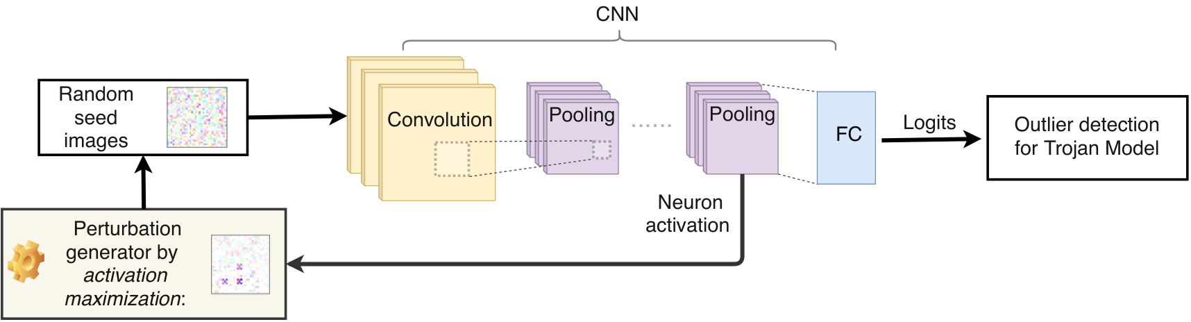
The previously introduced data-limited TrojanNet detector requires to access clean data of all $K$ classes. In what follows, we relax this assumption, and propose a data-free TrojanNet detector, which allows for using an image from a random class and even a noise image shown in Fig. 2. The framework is summarized in Fig. 3 (b), and details are provided in what follows.

It was previously shown in [7, 36] that a TrojanNet exhibits an unexpectedly high neuron activation at certain coordinates. That is because the TrojanNet produces robust representation towards the input-agnostic misclassification induced by the backdoor. Given a clean data $\mathbf{x}$, let $r_{i}(\mathbf{x})$ denote the $i$th coordinate of neuron activation vector. Motivated by [10, 11], we study whether or not an inverted image that maximizes neuron activation is able to reveal the characteristics of the Trojan signature from model weights. We formulate the inverted image as $\hat{\mathbf{x}}(\mathbf{m},\boldsymbol{\delta})$ in (1), parameterized by the pixel-level perturbations $\boldsymbol{\delta}$ and the binary mask $\mathbf{m}$ with respect to $\mathbf{x}$. To find $\hat{\mathbf{x}}(\mathbf{m},\boldsymbol{\delta})$, we solve the problem of activation maximization

where the notations follow (3.2) except the newly introduced variables $\mathbf{w}$, which adjust the importance of neuron coordinates. Note that if $\mathbf{w}=\mathbf{1}/d$, then the first loss term in (3.3) becomes the average of coordinate-wise neuron activation. However, since the Trojan-relevant coordinates are expected to make larger impacts, the corresponding variables $w_{i}$ are desired for more penalization. In this sense, the introduction of self-adjusted variables $\mathbf{w}$ helps us to avoid the manual selection of neuron coordinates that are most relevant to the backdoor.

In order to build TrojanNet detectors in both data-limited and data-free settings, we need to solve a sparsity-promoting optimization problem, in the specific forms of (3.2), (3.2), and (3.3), subject to a set of box and equality constraints. In what follows, we propose a general optimization method by leveraging the idea of proximal gradient [2, 26].

Consider a problem with the generic form of problems (3.2), (3.2), and (3.3),

where $F(\boldsymbol{\delta},\mathbf{m},\mathbf{w})$ denotes the smooth loss term, and $\mathcal{I}(\mathbf{x})$, $I^{\prime}(\mathbf{w})$ denote the indicator functions to encode the hard constraints

In $\mathcal{I}(\mathbf{x})$, $\alpha=1$ for $\mathbf{m}$ and $\alpha=255$ for $\boldsymbol{\delta}$. We remark that the binary constraint $\mathbf{m}\in\{0,1\}^{n}$ is relaxed to a continuous probabilistic box $\mathbf{m}\in[0,1]^{n}$.

To solve problem (11), we adopt the alternative proximal gradient algorithm [2], which splits the smooth-nonsmooth composite structure into a sequence of easier problems that can be solved more efficiently or even analytically. To be more specific, we alternatively perform

where $\mu_{t}$ denotes the learning rate at iteration $t$, and $\mathrm{Prox}_{\mu g}(\mathbf{a})$ denotes the proximal operator of function $g$ with respect to the parameter $\mu$ at an input $\mathbf{a}$.

We next elaborate on the proximal operators used in (13)-(15). The proximal operator $\mathrm{Prox}_{\mu_{t}(\mathcal{I}+\lambda\|\cdot\|_{1})}(\mathbf{a})$ is given by the solution to the problem

where $\mathbf{a}\mathrel{\mathop{:}}=\mathbf{m}^{(t)}-\mu_{t}\nabla_{\mathbf{m}}F(\boldsymbol{\delta}^{(t)},\mathbf{m}^{(t)})$. The solution to problem (16), namely, ${\mathbf{m}}^{(t+1)}$ is given by [2]

where ${m}^{(t+1)}_{i}$ dentoes the $i$th entry of $\mathbf{m}^{(t+1)}$, and $\mathrm{Clip}_{[0,1]}$ is a clip function that clip the variable to 1 if it is larger than 1 and to 0 if it is smaller than 0. Similarly, ${\boldsymbol{\delta}}^{(t+1)}$ in (14) is obtained by

where $\mathbf{b}\mathrel{\mathop{:}}=\boldsymbol{\delta}^{(t)}-\mu_{t}\nabla_{\boldsymbol{\delta}}F(\boldsymbol{\delta}^{(t)},\mathbf{m}^{(t+1)})$.

The proximal operator $\mathrm{Prox}_{\mu_{t}\mathcal{I}^{\prime}}(\mathbf{c})$ in (15) is given by the solution to the problem

which is equivalent to

Here $\mathbf{c}\mathrel{\mathop{:}}=\mathbf{w}^{(t)}+\mu_{t}\nabla_{\mathbf{w}}F(\delta^{(t+1)},\mathbf{m}^{(t+1)},\mathbf{w}^{(t)})$. The solution to problem (20) is given by [26]

where $[a]_{+}$ denotes the operation of $\max\{0,a\}$, and $\mu$ is the root of the equation $\mathbf{1}^{T}\left[\mathbf{c}-\mu\mathbf{1}\right]_{+}=\sum_{i}\max\{0,c_{i}-\mu\}=1.$

Substituting (17), (18) and (21) into (13)-(15), we then obtain the complete algorithm, in which each step has a closed-form.

Trojan settings. Testing models include VGG16 [32], ResNet-50 [16], and AlexNet [20]. Datasets include CIFAR-10 [19], GTSRB [33], and Restricted ImageNet (R-ImgNet) (restricting ImageNet [9] to $9$ classes). We trained 85 TrojanNets and 85 clean networks, respectively. The numbers of different models are shown in Table 6. Fig. 1 (a)-(f) show the CIFAR-10 and GTSRB dataset with triggers of dot, cross, and triangle, respectively. One of these triggers is used for poisoning the model. We also test models poisoned for two target labels simultaneously: the dot trigger is used for one target label, and the cross trigger corresponds to the other target label. Fig. 1 (g)-(i) show poisoned ImageNet samples with the watermark as the trigger. The TrojanNets are various by specifying triggers with different shapes, colors, and positions. The data poisoning ratio also varies from $10\%-12\%$. The cleanNets are trained with different batches, iterations, and initialization. Table 7 summarizes test accuracies and attack success rates of our generated Trojan and cleanNets. We compare DL-TND with the baseline Neural Cleanse (NC) [36] for detecting TrojanNets.

We plot the ROC curve of the “Total” in Fig. 5. The results show that DL-TND can perform well across different datasets and model architectures. Moreover, fixing $I^{(k)}$ as median, $T_{1}=0.54\sim 0.896$ could provide a detection success rate over $76.5\%$ for TrojanNets and a detection success rate over $82\%$ for cleanNets. Table 3 shows the comparisons of DL-TND to Neural Cleanse (NC) [36] on TrojanNets and cleanNets ($T_{1}=0.7$). Even using the MAD method as the detection rule, we find that DL-TND greatly outperforms NC in detection tasks of both TrojanNets and cleanNets (Note that NC also uses MAD). The results are shown in Table 8.

Results are summarized in Table 4, and the ROC curves are shown in Fig. 15.

First, we apply DL-TND and DF-TND on detecting TrojanNets with different levels attack success rate (ASR). We control ASR by choosing different data poisoning ratios when generating a TrojanNet. The results are summarized in Table 5. As we can see, our detectors can still achieve competitive performance when the attack likelihood becomes small, and DL-TND is better than DF-TND when ASR reaches $30\%$.

Moreover, we conduct experiments when the number of TrojanNets is much less than the total number of models, e.g., only $5$ out of $55$ models are poisoned. We find that the AUC value of the precision-recall curves are $0.97$ and $0.96$ for DL-TND and DF-TND, respectively. Similarly, the average AUC value of the ROC curves is $0.99$ for both detectors.

Third, we evaluate our proposed DF-TND to detect TrojanNets generalized by clean-label Trojan attacks [29]. We find that even in the least information case, DF-TND can still yield $0.92$ AUC score when detecting $20$ TrojanNets from $40$ models.

References

- [1] Model zoo, https://modelzoo.co/
- [2] Bolte, J., Sabach, S., Teboulle, M.: Proximal alternating linearized minimization for nonconvex and nonsmooth problems. Mathematical Programming 146(1-2), 459–494 (2014)
- [3] Carlini, N., Wagner, D.: Towards evaluating the robustness of neural networks. In: 2017 IEEE Symposium on Security and Privacy (SP). pp. 39–57. IEEE (2017)
- [4] Chen, B., Carvalho, W., Baracaldo, N., Ludwig, H., Edwards, B., Lee, T., Molloy, I., Srivastava, B.: Detecting backdoor attacks on deep neural networks by activation clustering. arXiv preprint arXiv:1811.03728 (2018)
- [5] Chen, H., Fu, C., Zhao, J., Koushanfar, F.: Deepinspect: a black-box trojan detection and mitigation framework for deep neural networks. In: Proceedings of the 28th International Joint Conference on Artificial Intelligence. pp. 4658–4664. AAAI Press (2019)
- [6] Chen, X., Liu, C., Li, B., Lu, K., Song, D.: Targeted backdoor attacks on deep learning systems using data poisoning. arXiv preprint arXiv:1712.05526 (2017)
- [7] Cheng, H., Xu, K., Liu, S., Chen, P.Y., Zhao, P., Lin, X.: Defending against backdoor attack on deep neural networks. arXiv preprint arXiv:2002.12162 (2020)
- [8] Cohen, J., Rosenfeld, E., Kolter, Z.: Certified adversarial robustness via randomized smoothing. In: Proceedings of the 36th International Conference on Machine Learning. pp. 1310–1320 (2019)
- [9] Deng, J., Dong, W., Socher, R., Li, L.J., Li, K., Fei-Fei, L.: Imagenet: A large-scale hierarchical image database. In: 2009 IEEE conference on computer vision and pattern recognition. pp. 248–255. Ieee (2009)
- [10] Engstrom, L., Ilyas, A., Santurkar, S., Tsipras, D., Tran, B., Madry, A.: Learning perceptually-aligned representations via adversarial robustness. arXiv preprint arXiv:1906.00945 (2019)
- [11] Fong, R., Patrick, M., Vedaldi, A.: Understanding deep networks via extremal perturbations and smooth masks. In: Proceedings of the IEEE International Conference on Computer Vision. pp. 2950–2958 (2019)
- [12] Gao, Y., Xu, C., Wang, D., Chen, S., Ranasinghe, D.C., Nepal, S.: Strip: A defence against trojan attacks on deep neural networks. In: Proceedings of the 35th Annual Computer Security Applications Conference. pp. 113–125 (2019)
- [13] Goodfellow, I.J., Shlens, J., Szegedy, C.: Explaining and harnessing adversarial examples (2014)
- [14] Gu, T., Dolan-Gavitt, B., Garg, S.: Badnets: Identifying vulnerabilities in the machine learning model supply chain. arXiv preprint arXiv:1708.06733 (2017)
- [15] Guo, W., Wang, L., Xing, X., Du, M., Song, D.: Tabor: A highly accurate approach to inspecting and restoring trojan backdoors in ai systems. arXiv preprint arXiv:1908.01763 (2019)
- [16] He, K., Zhang, X., Ren, S., Sun, J.: Deep residual learning for image recognition. In: Proceedings of the IEEE conference on computer vision and pattern recognition. pp. 770–778 (2016)
- [17] Kalchbrenner, N., Grefenstette, E., Blunsom, P.: A convolutional neural network for modelling sentences. arXiv preprint arXiv:1404.2188 (2014)
- [18] Kolouri, S., Saha, A., Pirsiavash, H., Hoffmann, H.: Universal litmus patterns: Revealing backdoor attacks in cnns. In: Proceedings of the IEEE/CVF Conference on Computer Vision and Pattern Recognition. pp. 301–310 (2020)
- [19] Krizhevsky, A., Hinton, G., et al.: Learning multiple layers of features from tiny images. Tech. rep., Citeseer (2009)
- [20] Krizhevsky, A., Sutskever, I., Hinton, G.E.: Imagenet classification with deep convolutional neural networks. In: Advances in neural information processing systems. pp. 1097–1105 (2012)
- [21] Kurakin, A., Goodfellow, I., Bengio, S.: Adversarial examples in the physical world. arXiv preprint arXiv:1607.02533 (2016)
- [22] Liu, Y., Lee, W.C., Tao, G., Ma, S., Aafer, Y., Zhang, X.: Abs: Scanning neural networks for back-doors by artificial brain stimulation. In: Proceedings of the 2019 ACM SIGSAC Conference on Computer and Communications Security. pp. 1265–1282 (2019)
- [23] Liu, Y., Ma, S., Aafer, Y., Lee, W.C., Zhai, J., Wang, W., Zhang, X.: Trojaning attack on neural networks (2017)
- [24] Madry, A., Makelov, A., Schmidt, L., Tsipras, D., Vladu, A.: Towards deep learning models resistant to adversarial attacks. arXiv preprint arXiv:1706.06083 (2017)
- [25] Moosavi-Dezfooli, S.M., Fawzi, A., Fawzi, O., Frossard, P.: Universal adversarial perturbations. In: Proceedings of the IEEE conference on computer vision and pattern recognition. pp. 1765–1773 (2017)
- [26] Parikh, N., Boyd, S., et al.: Proximal algorithms. Foundations and Trends® in Optimization 1(3), 127–239 (2014)
- [27] Peri, N., Gupta, N., Ronny Huang, W., Fowl, L., Zhu, C., Feizi, S., Goldstein, T., Dickerson, J.P.: Deep k-nn defense against clean-label data poisoning attacks. arXiv pp. arXiv–1909 (2019)
- [28] Ren, S., He, K., Girshick, R., Sun, J.: Faster r-cnn: Towards real-time object detection with region proposal networks. In: Advances in neural information processing systems. pp. 91–99 (2015)
- [29] Shafahi, A., Huang, W.R., Najibi, M., Suciu, O., Studer, C., Dumitras, T., Goldstein, T.: Poison frogs! targeted clean-label poisoning attacks on neural networks. In: Advances in Neural Information Processing Systems. pp. 6103–6113 (2018)
- [30] Shafahi, A., Najibi, M., Ghiasi, M.A., Xu, Z., Dickerson, J., Studer, C., Davis, L.S., Taylor, G., Goldstein, T.: Adversarial training for free! In: Advances in Neural Information Processing Systems. pp. 3353–3364 (2019)
- [31] Shen, Y., Sanghavi, S.: Learning with bad training data via iterative trimmed loss minimization. In: International Conference on Machine Learning. pp. 5739–5748 (2019)
- [32] Simonyan, K., Zisserman, A.: Very deep convolutional networks for large-scale image recognition. arXiv preprint arXiv:1409.1556 (2014)
- [33] Stallkamp, J., Schlipsing, M., Salmen, J., Igel, C.: Man vs. computer: Benchmarking machine learning algorithms for traffic sign recognition. Neural networks 32, 323–332 (2012)
- [34] Szegedy, C., Zaremba, W., Sutskever, I., Bruna, J., Erhan, D., Goodfellow, I., Fergus, R.: Intriguing properties of neural networks. 2014 ICLR arXiv preprint arXiv:1312.6199 (2014)
- [35] Tran, B., Li, J., Madry, A.: Spectral signatures in backdoor attacks. In: Advances in Neural Information Processing Systems. pp. 8000–8010 (2018)
- [36] Wang, B., Yao, Y., Shan, S., Li, H., Viswanath, B., Zheng, H., Zhao, B.Y.: Neural cleanse: Identifying and mitigating backdoor attacks in neural networks. Neural Cleanse: Identifying and Mitigating Backdoor Attacks in Neural Networks p. 0 (2019)
- [37] Xiang, Z., Miller, D.J., Kesidis, G.: Revealing backdoors, post-training, in dnn classifiers via novel inference on optimized perturbations inducing group misclassification. In: ICASSP 2020-2020 IEEE International Conference on Acoustics, Speech and Signal Processing (ICASSP). pp. 3827–3831. IEEE (2020)
- [38] Xie, C., Huang, K., Chen, P.Y., Li, B.: DBA: Distributed backdoor attacks against federated learning. In: International Conference on Learning Representations (2020)
- [39] Xu, X., Wang, Q., Li, H., Borisov, N., Gunter, C.A., Li, B.: Detecting ai trojans using meta neural analysis. arXiv preprint arXiv:1910.03137 (2019)
- [40] Yao, Y., Li, H., Zheng, H., Zhao, B.Y.: Latent backdoor attacks on deep neural networks. In: Proceedings of the 2019 ACM SIGSAC Conference on Computer and Communications Security. pp. 2041–2055 (2019)
- [41] Zhang, D., Zhang, T., Lu, Y., Zhu, Z., Dong, B.: You only propagate once: Accelerating adversarial training via maximal principle. In: Advances in Neural Information Processing Systems. pp. 227–238 (2019)
- [42] Zhang, H., Yu, Y., Jiao, J., Xing, E., Ghaoui, L.E., Jordan, M.: Theoretically principled trade-off between robustness and accuracy. In: Proceedings of the 36th International Conference on Machine Learning. pp. 7472–7482 (2019)
- [43] Zhao, P., Chen, P.Y., Das, P., Ramamurthy, K.N., Lin, X.: Bridging mode connectivity in loss landscapes and adversarial robustness. In: International Conference on Learning Representations (2020)
- [44] Zhu, C., Huang, W.R., Li, H., Taylor, G., Studer, C., Goldstein, T.: Transferable clean-label poisoning attacks on deep neural nets. In: Proceedings of the 36th International Conference on Machine Learning. pp. 7614–7623 (2019)
Appendix 0.A Data-Limited TrojanNet Detector (DL-TND)
Visualization of neuron activation. DL-TND tests all the labels (classes) by calculating one universal perturbation and multiple per-image perturbations for each label. Each data sample can obtain a neuron activation vector with the universal perturbation and a neuron activation vector with its per-image perturbation. In Fig. 7, we show the neuron activation of five data samples with universal perturbations and per-image perturbations under a target label, a non-target label, and a label in a clean network (cleanNet). The output magnitude for each coordinate is represented using gray scale. One can see that the strong similarities only appear under the target label, which supports our motivation for the DL-TND.
Neuron activation
(Universal)
(Per-image)
Target label
Non-target label
Label in cleanNet
Detection rule using median absolute deviation. Instead of using the detection rule in the main body of the paper, we can also employ the median absolute deviation (MAD) method. By MAD, if a single value in the -th position of is larger than (provide confidence rate), the network is poisoned and label is a target label, where . represents the absolute value. is the median of values in a vector. We compare DL-TND to Neural Cleanse (NC) [36] in Table 8 using MAD as the detection rule.
Appendix 0.B Data-Free TrojanNet Detector (DF-TND)
Visualization of logits output increase. Fig. 9 and 9 visualize the change of the logits output of 10 data samples under a cleanNet and a TrojanNet when label 4 (lab4) is the target label. One can see that the minimum increase belonging to the target label is while the maximum increase for labels in the cleanNet is . This large gap suggests that TrojanNets can be detected by properly selecting and there exists a wide selection range, implying the stability of our method.
Appendix 0.C DL-TND: Additional Experiments
Models for testing. Table 6 shows the numbers of different models used for testing. Models have three different architectures and are applied to CIFAR-10, GTSRB, and R-ImgNet. We trained TrojanNets and cleanNets, respectively. In addition to the diversity of model architecture and dataset types, we also train TrojanNets with different triggers. Table 7 shows the smallest test accuracy and attack success rate for TrojanNets and cleanNets. TrojanNets can reach a similar test accuracy as cleanNets while still keeping the high attack success rate. This suggests that they are valid TrojanNets as defined in Sec. 2.1.