Probing Reionization and Early Cosmic Enrichment with the Mg II Forest2020Probing Reionization and Early Cosmic Enrichment with the Mg II Forest–References

To simulate the Mg ii forest we need to model the distribution of metals in the IGM during the reionization phase transition. This is clearly an extreme challenge to simulate, as one must capture not only the physical state of the reionizing IGM, but also the production and dispersal of metals, and their ionization state. While progress on simulating all of this complex physics has been made in recent years (Oppenheimer et al. 2009; Pallottini et al. 2014; Pawlik et al. 2017; Jaacks et al. 2018; Jaacks et al. 2019; Doughty & Finlator 2019; Kirihara et al. 2020, e.g.), our goal here is to investigate detectability and perform a sensitivity analysis. To this end we adopt a highly simplistic toy model whereby the entire IGM is suffused with metals at a fixed metallicity $Z$ with solar relative abundances.

While in principle ionization corrections would be required to determine the fraction of Mg in the Mg ii state, this can be trivially simplified. Note that ionization edge of Mg i is at 0.56 Rydberg which lies below the 1 Rydberg ionizing edge for hydrogen, whereas the Mg ii edge is at 1.11 Rydberg blueward of the Lyman edge. The IGM is thus essentially completely transparent at the energies that ionize neutral Mg, and it is expected that even prior to reionization, the ultraviolet radiation field sourced by cosmic star-formation will produce a metagalactic UV background sufficiently intense at the Mg i edge to ionize all Mg into the Mg ii state. We explicitly checked this by running a CLOUDY (Ferland et al. 2017) model with gas at the mean density of the IGM at $z=7.5$ subjected to a Haardt & Madau 2012 UV background truncated at energies greater than 1 Rydberg. We find negligible $\lesssim 10^{-8}$ abundance of Mg in any ionization state besides Mg ii irrespective of the total $N_{\rm H}$ used to set the so-called stopping criterion. Thus for the purposes of the present study it is an excellent approximation to assume that the ionization state of Mg is simply tied to that of hydrogen, and neutral regions of the Universe are in the Mg ii state.

Having described our model of the metallicity and ionization state of Mg, we now turn to modeling the IGM during reionization. It is well known that reionization photoheating modifies the small-scale structure of the IGM. Although baryons trace dark matter fluctuations on large scales, on smaller scales gas is supported against gravitational collapse by thermal pressure. Analogous to the classic Jeans argument, baryonic fluctuations are suppressed relative to the pressureless dark matter, and gas is ‘pressure smoothed’ or ‘filtered’ on small scales (Gnedin & Hui 1998; Kulkarni et al. 2015; Rorai et al. 2017). As a result, the small-scale structure or clumpiness of the pre-reionization IGM is intimately related to its thermal evolution. It is currently unknown whether the IGM adiabatically cooled to extremely low temperatures $T\lesssim 1\,{\rm K}$ just before reionization at $z\sim 7-8$, or if a metagalactic X-ray background, sourced by faint AGN (Madau et al. 2004; Ricotti & Ostriker 2004), X-ray binaries (Madau & Fragos 2017), or PopIII stellar remnants (Xu et al. 2016), photoelectrically heated it to much higher temperatures $T\sim 1000\,{\rm K}$ (e.g. Furlanetto 2006b, but see Fialkov et al. 2014). During reionization ionization fronts propagate supersonically through the IGM, impulsively heating reionized gas to $\sim 10^{4}~{\rm K}$. This rapid temperature increase drives the Jeans scale from $\sim 1~{\rm ckpc}$ (for $T\lesssim 1~{\rm K}$) up to $\sim 100~{\rm ckpc}$, dissipating pre-reionization IGM small-scale structure on a timescale of $\sim 1~{\rm Gyr}$ (D’Aloisio et al. 2020; Davies & Hennawi 2020).

Since the Mg ii forest absorption arises from neutral regions of the IGM, in principle predicting its clustering strength depends on the small-scale structure of the IGM, and hence on the pre-reionization IGM temperature evolution. Accurately simulating the pre-reionization IGM is a daunting numerical problem (D’Aloisio et al. 2020; Davies & Hennawi 2020). Ideally, the simulation domain would be sufficiently large ($\gtrsim 10\,{\rm cMpc}$) to remain linear in its fundamental mode, and encompass the $768\,{\rm km\,s^{-1}}$ ($6.9~{\rm cMpc}$) doublet separation of Mg ii and typical size ($\sim 10~{\rm cMpc}$) of ionized bubbles, while simultaneously resolving the extremely small $\sim 1~{\rm ckpc}$ Jeans scale corresponding to the potentially very low temperatures $T\lesssim 1~{\rm K}$ prevailing in the pre-reionization IGM. Naively, this would require a $\sim 20,000^{3}$ grid or comparable number of SPH particles, unattainable even with the world’s largest supercomputers. Given our lack of knowledge of pre-reionization IGM temperature evolution, and the numerical challenge, we will utilize a snapshot of a hydrodynamical simulation at $z=7.5$ prior to reionization photoheating. This simulation, of a $L_{\rm box}=40\,{h^{-1}\,{\rm cMpc}}$ ($v_{\rm box}\equiv aH(z)L_{\rm box}=6600~{\rm km~s^{-1}}$ at $z=7.5$) domain on a $2048^{3}$ grid, has a grid scale of $29\,{\rm ckpc}$ ($3.2~{\rm km~s^{-1}}$), which would fail to resolve the $\sim 1~{\rm ckpc}$ Jeans scale for pre-reionization IGM temperatures $T\lesssim 1~{\rm K}$, but marginally resolve the $\sim 30~{\rm ckpc}$ Jeans scale if an X-ray background preheated the IGM to $T\sim 1000\,{\rm K}$.

As this paper focuses on the clustering of the Mg ii forest which is tied to the clustering of the IGM via our simple enrichment model, a discussion of the impact of this unresolved structure on our results is in order. Unlike the Gunn-Peterson optical depth for H i Ly$\alpha$ absorption, which probes neutral gas in an ionized medium and hence scales $\tau_{\rm Ly\alpha}\propto n_{\text{H\,{i}}}\propto n_{\rm H}^{2}$ quadratically with density, the analogous optical depth for the Mg ii forest $\tau_{\text{Mg\,{ii}}}\propto n_{\text{Mg\,{ii}}}\propto n_{\text{H\,{i}}}\propto n_{\rm H}$ scales only linearly with density, because the medium is predominantly neutral. Thus if $F=e^{-\tau_{\text{Mg\,{ii}}}}$, $\delta_{f}\equiv(F-\langle F\rangle)/\penalty\langle F\rangle\approx\tau_{\text{Mg\,{ii}}}\propto n_{\rm H}$ is always a good approximation for the small optical depths we consider, the Mg ii forest flux correlation function, $\xi_{\text{Mg\,{ii}}}\equiv\langle\delta_{f}\delta_{f}\rangle\propto\xi_{\rm\rho,1D}$, is simply proportional to the correlation function of the overdensity projected along skewers, which can in turn be written as the Fourier transform

of the analogous 1D density dimensionless power spectrum $\Delta_{\rm\rho,1D}^{2}(k)\equiv kP_{\rm\rho,1D}(k)/\penalty\pi$. The dimensionless power $\Delta_{\rho,1D}^{2}(k)$ is a smoothly rising function that traces the underlying clustering of the CDM, but is truncated by a sharp cutoff at the Jeans scale of the pre-reionization IGM. Failure to resolve this Jeans scale would then effectively truncate $\Delta_{\rm\rho,1D}^{2}(k)$ at the simulation grid scale $k_{\rm trunc}\simeq 2\pi/\penalty r_{\rm grid}$. Note that the $\cos(kr)$ factor in eqn. (1) implies that only wavenumbers with $kr\lesssim 1$ for which $\cos(kr)\sim 1$ contribute significantly to the integral, whereas wavenumbers $kr\gg 1$ contribute negligibly because of cancellations induced by the highly oscillatory $\cos(kr)$ term. In other words, only Fourier modes with wavelengths $\lambda\gtrsim r$ ($k\lesssim 2\pi/\penalty\lambda$) larger than the scale of interest contribute to the correlation function. Since the velocity separations (length scales) that we would realistically probe with real data ($\gtrsim 30~{\rm km~s^{-1}}$) correspond to spatial scales a least an order of magnitude larger than the pre-reionization IGM Jeans scale ($\sim 1-30~{\rm ckpc}$ or $\sim 0.1-3~{\rm km~s^{-1}}$), we do not expect this missing small-scale power to have a significant impact on our results.

We simulate the Mg ii forest using Nyx, a massively parallel N-body gravity + grid hydrodynamics code specifically designed for simulating the IGM (Almgren et al. 2013; Lukić et al. 2015). Initial conditions were generated using the music code (Hahn & Abel 2011) using a transfer function generated by camb (Lewis et al. 2000; Howlett et al. 2012). We assumed a $\Lambda$CDM cosmology with the following parameters: $\Omega_{\rm m}=0.3192$, $\Omega_{\Lambda}=0.6808$, $\Omega_{\rm b}=0.04964$, $h=0.6704$, $\sigma_{8}=0.826$ and $n_{\rm s}=0.9655$ which agree with latest cosmological constrains from the CMB (Planck et al. 2018) within one sigma. We adopted hydrogen and helium mass abundances ($X_{\rm p}=0.76$ and $Y_{\rm p}=0.24$) in agreement with the recent CMB observations and Big Bang nucleosynthesis (Coc et al. 2014). We simulated a domain with a box size of $40~{\rm cMpc}~h^{-1}$ using a $2048^{3}$ grid, and the simulation was started at $z_{\rm ini}=159$.

We analyze a snapshot at $z=7.5$, which is prior to the redshift of reionization in this simulation. Specifically, hydrodynamical simulations like Nyx which do not attempt to model reionization (Oñorbe et al. 2017; Oñorbe et al. 2019, but see) typically treat reionization by assuming a spatially uniform, time-varying metagalactic UVB radiation field, input to the code as a list of photoionization and photoheating rates that vary with redshift. The simulation we analyze reionizes at $z=6.0$, which is to say that the UVB is turned on at this redshift, which occurs at a later time than the snapshot we analyze at $z=7.5$. For additional details about the numerical approach see Oñorbe et al. 2019. The simulation analyzed here is similar to the ‘flash’ reionization simulations in that paper, where flash refers to the fact that the UVB is abruptly turned on at $z=6.0$ causing the simulation to instantaneously reionize.

Our Nyx hydrodynamical simulation yields the baryon density, peculiar velocity, and temperature at each grid cell. The only other quantity required to simulate the Mg ii forest is the hydrogen neutral fraction $x_{\text{H\,{i}}}$. For this we must create a model of the global reionization topology in the simulation domain. To generate the H i neutral fraction $x_{\text{H\,{i}}}$ throughout the simulation we use a modified version of the semi-numerical reionization code 21cmFAST⁵⁵ 5 https://github.com/andreimesinger/21cmFAST (Mesinger et al. 2011), to be presented in further detail in Davies & Furlanetto (in prep.). The semi-numerical approach computes the fraction of material that has collapsed into dark matter halos, $f_{\rm coll}$, following conditional Press-Schechter (Lacey & Cole 1993) applied to an approximate non-linear density field computed by applying the Zel’dovich approximation (Zel’Dovich 1970) to the initial conditions of the Nyx simulation, and evolving it to $z=7.5$. A region is considered ionized if $f_{\rm coll}>\zeta^{-1}$ on any scale, where $\zeta$ is the “ionizing efficiency," which combines several parameters governing the efficiency of star formation and the production and escape of ionizing photons from galaxies into a single parameter that corresponds to the total number of ionizing photons emitted per collapsed baryon. An ionizing mean free path $\lambda_{\rm mfp}$ is implemented by suppressing the contribution of ionizing photons with a smooth exponential decline rather than the traditional hard cutoff ($R_{\rm max}$). The neutral fraction $x_{\text{H\,{i}}}$ is computed on a $256^{3}$ grid encompassing the Nyx simulation domain, which is chosen to be sufficiently fine to sample the ionization topology but also coarse enough to guarantee sufficient numbers of dark matter halos (which source the ionizing photons) in each cell.

We generated a sequence of 51 different reionization topologies, parameterized by the volume filling fraction of neutral hydrogen $\langle x_{\text{H\,{i}}}\rangle$ at $z=7.5$, spanning the range $\langle x_{\text{H\,{i}}}\rangle$ = 0.0 to 1.0 in steps of 0.02. The models used here adopted an ionizing photon mean free path $\lambda_{\rm mfp}=20~{\rm cMpc}$, and the ionizing efficiency was then adjusted to get the full range of $\langle x_{\text{H\,{i}}}\rangle$ required. For additional details about the semi-numerical reionization model see Davies et al. 2018b, Oñorbe et al. 2019, and Davies & Furlanetto, in prep.

To simulate the Mg ii forest we generate skewers by drawing random locations along one face of the simulation cube, and record the baryon density, the line-of-sight component of the peculiar velocity field, the temperature, and neutral fraction at each line-of-sight location in the grid, where the latter comes from the semi-numerical reionization topology just described. The doublet nature of the Mg ii ion requires that we deal with resonant absorption at two wavelengths $\lambda 2796,\lambda 2804$Å , which corresponds to a velocity difference of $\Delta v=768~{\rm km~s^{-1}}$. In practice we compute the optical depth $\tau_{2796}$ for the stronger $\lambda 2796$ transition, and then rescale this array by the oscillator strength ratio of $f_{2804}/f_{2796}=0.497$ to obtain $\tau_{2804}$, which we shift by the doublet separation $\Delta v$, allowing us to compute the total optical depth $\tau_{\text{Mg\,{ii}}}=\tau_{2796}+\tau_{2804}$. Below we describe our approach for generating skewers of $\tau_{2796}$, the optical depth in the $\lambda$2796Å  resonance.

The optical depth for resonant absorption for an ionic transition $X^{n+}$ of an element $X$ in its $n$th ionization state is

where $\nu$ is the frequency, $n_{X}$ is the number density of the element $X$, $x^{n+}$ is the fraction of this element populating the $n$th ionization state, and

is the frequency specific cross-section. Here $e$ and $m_{e}$ are the electron charge and mass, respectively, $c$ is the speed of light, $f_{\ell u}$ is the oscillator strength for the resonant transition $\ell\rightarrow u$ at rest-frame frequency $\nu_{\ell u}$, and $\phi_{\nu}$ is the line profile. Whereas in general $\phi_{\nu}$ is described by the Voigt profile, for the extremely low optical depths characterizing metal-line forests it is a very good approximation to represent $\phi_{\nu}$ with a Gaussian form

where $\Delta\nu_{D}=\left(b/\penalty c\right)\nu_{\ell u}$ is the Doppler frequency width of the Gaussian profile determined by the Doppler parameter $b=\sqrt{2k_{\rm B}T/\penalty m_{X}}$ characterizing thermal broadening of the absorption lines, where $k_{\rm B}$ is Boltzmann’s constant and $m_{\rm X}$ is the mass of element $X$.

If we assume, as we will throughout this work, that the metal line species $X$ is uniformly mixed with the baryons in the IGM, then we can write $n_{X}=\langle n_{\rm X}\rangle\Delta$, where $\Delta\equiv\rho_{\rm B}/\penalty\langle\rho_{\rm B}\rangle$, $\rho_{\rm B}$ is baryon mass density, angle brackets represent an average over the volume of the Universe, and $\langle n_{\rm X}\rangle=Z/\penalty Z_{\odot}\left(n_{\rm X}/\penalty n_{\rm H}\right)_{\odot}\langle n_{\rm H}\rangle$, where $Z/\penalty Z_{\odot}$ is the metallicity in solar units, and $\left(n_{\rm X}/\penalty n_{\rm H}\right)_{\odot}$ is the abundance of element $X$ in the sun.

Combining eqns. 2-4, and transforming to velocity coordinates using the Doppler formula $\nu^{\prime}=\nu_{\ell u}[1-(v^{\prime}-v)/\penalty c]$ and the Hubble relation $dr=dv/\penalty H(z)$, where $H(z)$ is the Hubble expansion rate at redshift $z$, we finally arrive at

where we have defined $\tau_{X,0}$ the metal-line forest analog of the Gunn-Peterson optical depth (Oh 2002),

or plugging in numbers for the Mg ii forest

where we used the Mg abundance $\left(n_{\rm Mg}/\penalty n_{\rm H}\right)_{\odot}=3.4\times 10^{-5}$ determined from the solar photosphere (Asplund et al. 2009), and the oscillator strength $f_{2796}$ and wavelength $\lambda_{\ell u}$ of the stronger Mg ii $\lambda 2796~$Å  transition.

Special attention must be paid to the construction of metal-line forest skewers because of the extremely small Doppler parameters $b$. This results from both cold pre-reionization IGM temperatures and the fact that metals are much heavier than hydrogen. The temperature of the pre-reionization IGM is currently unknown and could be anywhere in the range $T\sim 1-1000\,{\rm K}$, as discussed in § 2.1. Plugging in numbers for the Doppler parameter for an ion $X$

where we normalized using the atomic weight of Mg. The Nyx hydrodynamical simulations employed in this work have a grid scale of $dv=3.2\,{\rm km\,s^{-1}}$ at $z=7.5$, thus the thermal broadening of Mg ii forest absorption lines are far from being resolved by our native velocity grid. One option would be to interpolate the simulated density and temperature fields onto a much finer grid before performing the convolution in eqn. (5) required to construct simulated Mg ii forest skewers, but this is computationally intensive given the small $b$ parameters one would need to resolve. Instead, we adopt the clever approach described in Appendix B of Lukić et al. 2015, which is far faster because it enables one to work on the native grid, but nevertheless explicitly conserves optical depth. Specifically, we discretize the integral in eqn. (5), taking the overdensity and temperature as constant across each grid cell. For the $k$th pixel at velocity $v_{k}=kdv$ in the Hubble expansion, the optical depth is

where the error function⁶⁶ 6 Note that equivalent eqn. B5 in Lukić et al. 2015 is missing a factor of $1/\penalty 2$ results from the integral of the Gaussian profile across the $i$th pixel (from $v_{i-1/\penalty 2}$ to $v_{i+1/\penalty 2}$), and $y_{i-1/2}=(v_{j}-v_{\parallel,i}-v_{i-1/\penalty 2})/\penalty b$, where $v_{\parallel,i}$ is the component of the gas peculiar velocity parallel to the sightline, $v_{i-1/\penalty 2}=(i-1/\penalty 2)dv$, and an analogous expression holds for $y_{i+1/2}$.

Our goal is to construct a large set of Mg ii forest skewers for a model grid governed by two parameters, $[{\rm Mg/\penalty H}]$ and $\langle x_{\text{H\,{i}}}\rangle$. We start with 10,000 skewers of $\Delta$, $v_{\parallel}$, and $T$, extracted from the Nyx simulation at random locations along one face of the cube. For the $x_{\text{H\,{i}}}$ field, we use the set of 51 reionization topologies in the range $\langle x_{\text{H\,{i}}}\rangle=0.0$ to 1.0. Given that the Mg ii forest optical depth $\tau_{\text{Mg\,{ii}}}$ is linear in $Z$ (see eqn. 6), which we define as $Z/\penalty Z_{\odot}\equiv 10^{[{\rm Mg/\penalty H}]}$, we perform the convolutions in eqn. (9) for each value of $\langle x_{\text{H\,{i}}}\rangle$, but a single metallicity, and scale the resulting optical depth to the desired metallicity. For the metallicity grid we use 201 models spanning the range $[{\rm Mg/\penalty H}]=[-6.0,-2.0]$. The result of this procedure is a set of 10,000 Mg ii forest skewers generated for a grid of $51\times 201=10,251$ models.

For the purpose of visualizing real observational data and performing statistical inference we create mock spectra with smearing induced by finite spectral resolution and add noise consistent with a realistic ${\rm S/\penalty N}$ ratio. We parameterize the data quality with the FWHM of the spectral resolution assuming a Gaussian line spread function, and the ${\rm S/\penalty N}$ per pixel, where the spectral sampling is assumed to be $n_{\rm samp}=3$ pixels per spectral resolution element of width the FWHM. Our simulated spectra are convolved with a Gaussian consistent with the spectral resolution, interpolated onto a velocity grid set by the spectral sampling, and then Gaussian random noise is added with a standard deviation $\sigma_{\rm S/\penalty N}=({\rm S/\penalty N})^{-1}$.

For a quasar at $z=7.5$, and considering a redshift interval of $\Delta z=0.6$ from $z=6.9-7.5$ where we expect the Universe to be significantly neutral, the Mg ii forest is redshifted to observed frame wavelengths of $\lambda=2.21-2.38\mu{\rm m}$ in the $K$-band. In this work we model spectra from JWST/NIRSpec for which the sky background at the relevant wavelengths comes from zodiacal light and is relatively smooth. For this case, assuming spectral noise that is constant with wavelength is a reasonable approximation. On the other hand, ground-based observations of this spectral region would have heteroscedastic noise owing to the forest of atmospheric OH airglow lines. As we will aim to measure the two-point correlation function of the Mg ii forest (see § 3), formally the noise in the estimated correlation function averages to zero at all non-zero velocity lags irrespective of whether or not it is heteroscedastic. As such, even for ground-based observations, we do not expect the heteroscedasticity of the noise to be a significant issue⁷⁷ 7 This assumes that correlated noise resulting from sky subtraction systematics are insignificant, which we expect to be the case., provided that one take our assumed ${\rm S/\penalty N}$ ratio to be a suitable average over the spectral region in question.

We primarily focus on mock data with ${\rm FWHM}=100~{\rm km~s^{-1}}$ and ${\rm S/\penalty N}=100$, representative of what can be achieved with JWST/NIRSpec in a 10hr integration for a typical $z\gtrsim 7$ quasar with an AB apparent magnitude of $m_{\rm 1450}=20.5$, chosen to correspond to the observed frame $J$-band. This estimate is based on calculations performed with the JWST/NIRSpec exposure time calculator⁸⁸ 8 https://jwst.etc.stsci.edu/.

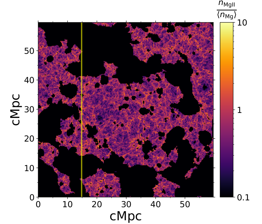
The topology of Mg ii absorbing gas predicted by our model is shown in Fig. 1 for a universe with a volume averaged neutral fraction $\langle x_{\text{H\,{i}}}\rangle=0.50$ at $z=7.5$. The figure shows a single pixel ($29~{\rm ckpc}$) slice through $x_{\text{H\,{i}}}\Delta$, which is equivalent to $n_{\text{Mg\,{ii}}}/\penalty\langle n_{\rm Mg}\rangle$ given our assumption of a uniform metallicity distribution and $x_{\text{H\,{i}}}=x_{\text{Mg\,{ii}}}$ (see § 2.1). The vertical yellow line shows a skewer through this volume taken to be the line-of-sight direction towards the observer. Fig. 2 shows our predictions for the Mg ii forest spectra along this sightline. The top panel shows the baryon overdensity, which traces the clumpy structure of the pre-reionization IGM determined by the underlying CDM as discussed in § 2.1. The second panel from the top shows the IGM neutral fraction, $x_{\text{H\,{i}}}$, from our semi-numerical reionization topology. The lower panels show the simulated Mg ii forest for various values of $[{\rm Mg}/\penalty{\rm H}]$, where the red curves are perfect spectra and black histograms show realistic mock JWST/NIRSpec spectra with a resolution ${\rm FWHM}=100~{\rm km~s^{-1}}$ and ${\rm S/\penalty N}=100$ per pixel (see § 2.6 for details).

The correlation function $\xi(\Delta v)$ is shown in Fig. 3 for several different combinations of metallicity, $[{\rm Mg}/\penalty{\rm H}]$, and volume averaged neutral fraction, $\langle x_{\text{H\,{i}}}\rangle$. For this computation we have assumed noiseless data, and a resolution of ${\rm FWHM}=30~{\rm km~s^{-1}}$ typical of a ground based echelle spectrograph.

There are several important features of the correlation function shown in Fig. 3 which we now describe. First, because pre-reionization IGM baryons trace the clumpy small-scale structure set by the underlying CDM, there is significant variance on small scales and as a result the Mg ii forest correlation function exhibits a precipitous rise towards small velocity lags. Second, there is a strong peak at the doublet separation $\Delta v_{\text{Mg\,{ii}}}=768\,{\rm km\,s^{-1}}$, indicated by the red vertical dashed line, which arises from the doublet nature of the Mg ii transition. The height of this peak is a result of the significant small-scale power, since pixels separated by around $\Delta v_{\text{Mg\,{ii}}}=768\,{\rm km\,s^{-1}}$ are in reality probing correlated fluctuations in the gas at much smaller velocity lags. Finally, at intermediate to large velocity lags $\xi(\Delta v)$ exhibits an overall power-law dependence on $\Delta v_{\text{Mg\,{ii}}}$, which appears to be highly sensitive to the value of $\langle x_{\text{H\,{i}}}\rangle$. This occurs because line-of-sight fluctuations in neutral fraction $x_{\text{H\,{i}}}$ (see Fig. 2 second panel from top) modulate the Mg ii forest sourcing fluctuations on a hierarchy of scales set by the topology of the neutral regions during reionization (see Fig. 1).

Naively one might expect a perfect degeneracy between the global neutral fraction $\langle x_{\text{H\,{i}}}\rangle$ and Mg abundance $[{\rm Mg}/\penalty{\rm H}]$, since the optical depth for the Mg ii forest in eqn. (5) depends on the degenerate product of $x_{\text{H\,{i}}}$ and $[{\rm Mg}/\penalty{\rm H}]$. However, this naive intuition proves incorrect, as is clear by comparing the solid, $\langle x_{\text{H\,{i}}}\rangle=0.9$, and dotted, $\langle x_{\text{H\,{i}}}\rangle=0.2$, curves in Fig. 3. At fixed $\langle x_{\text{H\,{i}}}\rangle$, the amplitude of the correlation function scales as the square of the Mg abundance $[{\rm Mg}/\penalty{\rm H}]$, as expected from eqn. (5) and eqn. (11) — when $F$ is small $|\delta_{f}|\approx|\tau-\langle\tau\rangle|$, and thus $\xi\propto\delta_{f}^{2}\propto\tau_{\text{Mg\,{ii}}}^{2}$. But the dependence of $\xi(\Delta v)$ on $x_{\text{H\,{i}}}$ is more complex, which probes large-scale $\sim 1-30~{\rm cMpc}$ fluctuations arising from the global topology of reionization.

In Fig. 4 we illustrate the impact of spectral resolution on $\xi(\Delta v)$ for a model with $[{\rm Mg}/\penalty{\rm H}]=-3.4$ and $\langle x_{\text{H\,{i}}}\rangle=0.2$. Finite spectral resolution smears out the small-scale structure in the Mg ii forest reducing the amount of variance at velocity lags smaller than the FWHM of the spectrograph. This is readily apparent from the curves in Fig. 4, where one sees that the rise in the correlation function has been smoothed out at velocity lags comparable to the spectral resolution. Because the peak in the correlation function at the doublet separation $\Delta v=768~{\rm km~s^{-1}}$ also results from small-scale correlations (see discussion in § 3.1), we observe that this peak is broadened by the spectral smearing and its resulting width is effectively determined by the spectral resolution. The black curves (labeled Perfect Spectrum) have not been explicitly smoothed to model spectral resolution, however the small-scale power is nevertheless be smoothed by the finite spatial resolution of our simulation, which has a grid scale of $29~{\rm ckpc}$ corresponding to $3.2{\rm km~s^{-1}}$ in the Hubble flow. As discussed in § 2.1, our simulations will not resolve the small-scale structure of the IGM if pre-reionization baryons are at temperature $T\lesssim 1000\,{\rm K}$ resulting in a Jeans scale smaller than our grid scale. However, we expect this smoothing to only impact the correlation function at velocity lags smaller than the grid scale $3.2~{\rm km~s^{-1}}$ (see eqn. 1). But measuring lags this small would require high-resolution near-IR spectra which we do not consider here.

We consider a realistic mock dataset of $n_{\rm QSO}=10$ quasar spectra, each covering a pathlength of $\Delta z=0.6$ of the Mg ii forest, resulting in a total pathlength of $\Delta z_{\rm tot}=n_{\rm QSO}\times\Delta z=6.0$. Our forward modeled spectra have a velocity extent of $6567~{\rm km~s^{-1}}$ set by how our simulation box fits onto the spectral velocity grid, which is far smaller than the $21,936~{\rm km~s^{-1}}$ corresponding to ⁹⁹ 9 For $\Delta z=0.6$ and $z=7.5$, we assume spectra covering the range $z=6.9-7.5$ centered at $z_{\rm eff}=7.2$, such that velocity interval covered is $c\Delta z/(1+z_{\rm eff})=21,936~{\rm km~s^{-1}}$ $\Delta z=0.6$. We thus create a mock dataset with the same effective pathlength by aggregating the equivalent integer number of shorter $6567~{\rm km~s^{-1}}$ skewers. In other words, we model our mock dataset comprising of $n_{\rm QSO}=10$ quasars with $\Delta z=0.6$ and desired pathlength of $\Delta z_{\rm tot}=6.0$, with an integer number of $n_{\rm path}=33$ skewers, corresponding to a slightly shorter pathlength of $\Delta z_{\rm tot}=5.93$. As described in § 2.6, we parameterize the data quality with the spectral resolution FWHM and the ${\rm S/\penalty N}$ ratio, and here consider observations with JWST/NIRSpec and assume FWHM=$100~{\rm km~s^{-1}}$ and ${\rm S/\penalty N}=100$.

Following standard practice for correlation function measurements, we adopt a multivariate Gaussian likelihood for the Mg ii forest correlation function

where $\mathbf{C}$ is the covariance matrix and $\mathbf{d}\equiv{\hat{\xi}}(\Delta v)-\xi(\Delta v|[{\rm Mg/\penalty H}],\langle x_{\text{H\,{i}}}\rangle)$, where ${\hat{\xi}}(\Delta v)$ is the correlation function estimated from the data and $\xi(\Delta v|[{\rm Mg/\penalty H}],\langle x_{\text{H\,{i}}}\rangle)$ is the parameter dependent model correlation function, which we will henceforth simply denote by $\xi(\Delta v)$. We compute the correlation function in $k=31$ linearly spaced velocity bins of equal width, which determines the dimensionality of $\mathbf{d}$ and $\mathbf{C}$. We choose the bin width to match our resolution of $100~{\rm km~s^{-1}}$, and the bin centers extend from velocity lags $80~{\rm km~s^{-1}}$ to $3080~{\rm km~s^{-1}}$. From our ensemble of 10,000 skewers we compute the average value of $\xi(\Delta v)$ at each location on our 2D grid ($51\times 201$) of $\langle x_{\text{H\,{i}}}\rangle$ and $[{\rm Mg/\penalty H}]$ models.

Typically the covariance matrix is either determined from the data itself, via i.e. a bootstrap procedure, or synthesized from forward models. Given the relatively small mock dataset that we consider $n_{\rm QSO}=10$ or $\Delta z_{\rm tot}=6.0$, the covariance estimated from the data would be too noisy so we adopt the latter approach. The covariance matrix is defined via

where the indices $i$ and $j$ denote bins of velocity lag $\Delta v$, and the angle brackets denote the average over an ensemble of mock realizations of the dataset in question, which in this case is a correlation function ${\hat{\xi}}(\Delta v)$ computed from a set of $n_{\rm path}=33$ skewers. Note that this covariance matrix depends on the model parameters ($\langle x_{\text{H\,{i}}}\rangle,[{\rm Mg/\penalty H}]$). For each model in our $51\times 201$ grid, we generate $10^{6}$ mock datasets by grabbing $n_{\rm path}=33$ random skewers from our sample of 10,000 without replacement, and computing their average correlation function ${\hat{\xi}}(\Delta v)$, allowing us to estimate the covariance from eqn. (13).

A useful tool for visualizing the covariance structure is the correlation matrix defined by

Fig. 5 shows an example correlation matrix for a model with $\langle x_{\text{H\,{i}}}\rangle=0.74$ and $[{\rm Mg/\penalty H}]=-3.7$. The diagonal band structure of the correlation matrix can be easily understood. By definition the correlation matrix is unity along the diagonal. The other two prominent sidebands result from correlations induced by the doublet nature of Mg ii, i.e. a fluctuation in $\xi(\Delta v)$ in a bin at $\Delta v=1200~{\rm km~s^{-1}}$ will preferentially correlate with fluctuations in velocity bins at $\Delta v=1200\pm 768\,{\rm km\,s^{-1}}$. Finally, the steep rise of the correlation function towards zero-lag and its ‘mirror image’ at $\Delta v=768\,{\rm km\,s^{-1}}$ (see Fig. 3), implies correlation function estimates at small velocity lags correlate more strongly with each other. For example the correlation function bin at $\Delta v=500~{\rm km~s^{-1}}$, which is $268~{\rm km~s^{-1}}$ away from the doublet peak at $\Delta v=768\,{\rm km\,s^{-1}}$, actually contains contributions from the same structures producing the small-scale rise of the correlation function towards zero lag at velocity $\Delta v=268~{\rm km~s^{-1}}$, resulting in a high value for the correlation matrix $\simeq 0.6$. These effects conspire to produce the high level of correlations along the ‘base’ of the ‘trident’ extending diagonally across the correlation matrix at small velocity lags.

Finally, we note that the ‘zero-lag’ $\xi(\Delta v)$ bin is completely omitted from our inference calculations. Although in principle this bin contains information, utilizing it would require that one subtract off the noise variance. Our $1\sigma$ noise level per spectral pixel is $1\%$, whereas the standard deviation of the Mg ii forest per spectral pixel is $0.5\%$ for a model with $\langle x_{\text{H\,{i}}}\rangle=0.74$ and $[{\rm Mg/\penalty H}]=-3.7$, and scales as roughly metallicity squared (see discussion in § 3.1). Thus using the ‘zero-lag’ bin would presume that one can determine the absolute noise level to exquisite accuracy, whereas using non-zero lags assumes that the noise correlations are much smaller than the signal correlations, which is a far weaker assumption given that the noise is expected to be white.

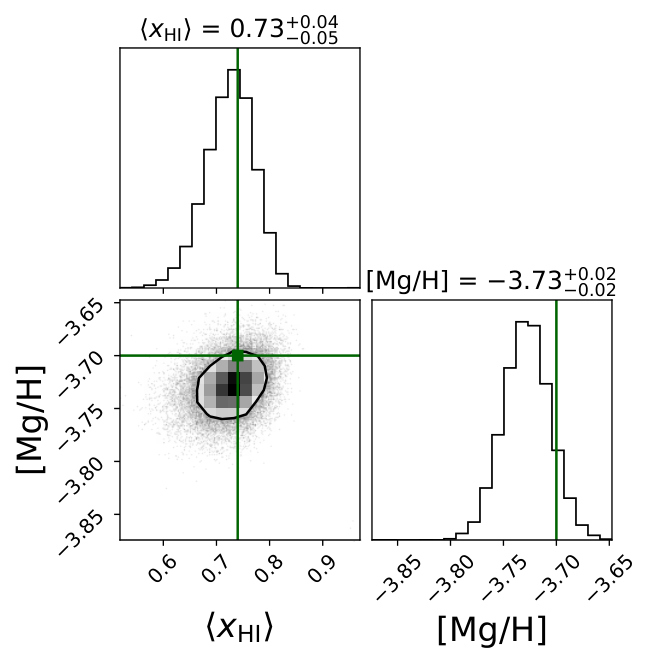
Given our mock JWST dataset of $n_{\rm QSO}=10$ quasars (FWHM=$100~{\rm km~s^{-1}}$ and ${\rm S/\penalty N}=100$, see § 2.6 and Fig. 2) we can use the likelihood in eqn. (12) to perform Markov Chain Monte Carlo (MCMC) parameter inference. We assume a flat linear prior on the volume averaged neutral fraction extending from $x_{\text{H\,{i}}}=[0.0,1.0]$, and a flat prior in the $\log_{10}$ of the Mg abundance from $[{\rm Mg}/\penalty{\rm H}]=[-6.0,-2.0]$, i.e. our prior is uninformative and spans the parameter space covered by our model grid. For the fiducial model, we choose $[{\rm Mg}/\penalty{\rm H}]=-3.7$ and $x_{\text{H\,{i}}}=0.74$, where the former is motivated by IGM metallicity measurements at lower-$z$, and the latter by current reionization constraints from the CMB (Planck et al. 2018, e.g.), IGM damping wings towards $z\gtrsim 7$ quasars (Mortlock et al. 2011; Greig et al. 2017; Bañados et al. 2018; Davies et al. 2018b; Greig et al. 2019; Wang et al. 2020; Yang et al. 2020) and the disappearance of strong Ly$\alpha$ emission from galaxies (Mason et al. 2018; Mason et al. 2019; Hoag et al. 2019). The resulting mock correlation function and parameter constraints are shown in Fig. 6. Our analysis indicates that for this combination of model parameters one can simultaneously determine the Mg abundance $[{\rm Mg}/\penalty{\rm H}]$, with a $1\sigma$ precision of 0.02 dex, and measure the global neutral fraction $\langle x_{\text{H\,{i}}}\rangle$ to 5%.

The constraining power of the Mg ii correlation function, or more precisely the width and orientation of the contours in the $\langle x_{\text{H\,{i}}}\rangle$-$[{\rm Mg}/\penalty{\rm H}]$ plane in the right panel of Fig. 6, are a strong function of the true value of the parameters. We illustrate this dependence in Fig. 7, which shows the resulting 68% and 95% confidence intervals (colored lines) at a grid of values for the true model (indicated by filled circles) in the $\langle x_{\text{H\,{i}}}\rangle$-$[{\rm Mg}/\penalty{\rm H}]$ plane. For intermediate values of the neutral fraction $\langle x_{\text{H\,{i}}}\rangle\simeq 0.5$ and Mg abundances $[{\rm Mg}/\penalty{\rm H}]\gtrsim-4$, there is no significant degeneracy between the two parameters. At low $\langle x_{\text{H\,{i}}}\rangle\lesssim 0.1$ and high $\langle x_{\text{H\,{i}}}\rangle\gtrsim 0.9$ neutral fractions a degeneracy between the parameters starts to emerge. This degenerate behavior can be qualitatively understood as follows. For $\langle x_{\text{H\,{i}}}\rangle\lesssim 0.1$, the steepening power law shape of the correlation function washes out the peaks arising from small-scale structure toward both zero-lag and the doublet separation (see Fig. 3), particularly at JWST resolution (${\rm FWHM}=100~{\rm km~s^{-1}}$) where these peaks are smeared (see Fig. 4). In this regime the additional constraining power provided by these peaks is washed out, and the $[{\rm Mg}/\penalty{\rm H}]$ increases the roughly power-law correlation function amplitude, whereas $\langle x_{\text{H\,{i}}}\rangle$ alters its amplitude and slope, resulting in a degeneracy. The degeneracy at $\langle x_{\text{H\,{i}}}\rangle\gtrsim 0.9$ occurs for similar reasons. For these largely neutral models, the power-law behavior of the correlation (left panel of Fig. 3) due to the topology of reionization is suppressed, and all the signal is concentrated at small velocity lags and at the doublet separation. In this regime the naive degeneracy expected from the optical depth (see eqn. 5 and the discussion at the end of § 3.1) sets in, since the degenerate product of metallicity and neutral fraction determine the amplitude of fluctuations and hence the correlation function. This degeneracy is exacerbated by the fact that reionization occurs from the inside out, and at high values of $\langle x_{\text{H\,{i}}}\rangle$ the rare ionized patches will be co-spatial with the highest density gas. As a fully neutral Universe is approached $\langle x_{\text{H\,{i}}}\rangle\rightarrow 1$ these dense regions become neutral, and the amplitude of the correlation function will become hyper-sensitive to $\langle x_{\text{H\,{i}}}\rangle$ due to the outsize contribution of these dense regions to the fluctuations. Together we expect some degeneracy between $[{\rm Mg}/\penalty{\rm H}]$ and $\langle x_{\text{H\,{i}}}\rangle$ to emerge at high values $\langle x_{\text{H\,{i}}}\rangle\gtrsim 0.9$, and that a small change in $\langle x_{\text{H\,{i}}}\rangle$ can compensate for a relatively large change in $[{\rm Mg}/\penalty{\rm H}]$, which is exactly the behavior observed in Fig. 7.

It is conceivable that the neutral IGM is actually totally pristine, as would be the case if the metals produced by the star-formation that drives reionization remain highly concentrated around the galaxies producing them. In this scenario, we would obtain a null detection of the Mg ii forest correlation function even if the IGM were significantly neutral. Such a null detection would nevertheless provide an upper limit on the enrichment of the IGM during the EoR, providing an extremely interesting constraint on the enrichment history of the Universe. To quantify this, we assume that an independent constraint on the reionization history exists from other probes (e.g. CMB, IGM damping wings, Ly$\alpha$ disappearance in galaxies, or 21cm observations) such that $\langle x_{\text{H\,{i}}}\rangle>0.5$ at $z=7.5$. For our fiducial model we choose $[{\rm Mg}/\penalty{\rm H}]=-6.0$ (the lowest metallicity in our grid) and $x_{\text{H\,{i}}}=0.74$, which results in a correlation function effectively consistent with zero. We perform statistical inference via MCMC as before, but now adjust the prior to have $\langle x_{\text{H\,{i}}}\rangle>0.5$, and importantly, we adopt a linear prior on the Mg abundance to be in the range $10^{[{\rm Mg}/\penalty{\rm H}]}=[0.0,1.0]$. The reasoning behind changing the abundance prior to be linear, as opposed to the $\log_{10}$ prior adopted above, is that for a logarithmic prior, the resulting upper limit on $[{\rm Mg}/\penalty{\rm H}]$ would depend on the prior range adopted, whereas this is not the case with a linear prior. Marginalizing over the unknown neutral fraction with the MCMC samples, we find that a null correlation function detection from our mock dataset would place an upper limit on the Mg abundance of $[{\rm Mg}/\penalty{\rm H}]<-4.4$ at 95% confidence. This stringent limit is nearly 0.5 dex more sensitive than the most metal-poor Lyman Limit Systems (LLSs) and Damped Ly$\alpha$ Systems (DLAs) known (Fumagalli et al. 2011; Crighton et al. 2016; Cooke et al. 2017; Robert et al. 2019) and is in the realm of the alpha element abundances of the most metal-poor stars known (Frebel & Norris 2015). But whereas these metal-poor absorbers and stars constitute the rarest outliers from their respective parent populations, the sensitive Mg ii forest abundance constraint one would obtain is the average for the IGM as a whole.

To populate our simulated skewers with CGM absorbers we require the distribution function $\frac{d^{2}N}{dzdW_{\lambda}}$ of rest-frame equivalent width. Whereas studies sensitive to the strongest absorbers typically adopt an exponential form (Nestor et al. 2005; Chen et al. 2017, e.g.) for this distribution function, echelle based searches sensitive enough to detect weak Mg ii absorbers $W_{\lambda}\lesssim 0.1$ Å  find that a Schechter-like (Schechter 1976) function provides a better fit to the data (Kacprzak & Churchill 2011; Mathes et al. 2017),

which we will adopt here since, as we will see, only the weakest CGM absorbers are expected to significantly contaminate the Mg ii forest signal arising from the neutral IGM.

The abundance of weak absorbers at $z>6$ is currently not well constrained by observations. Chen et al. 2017 measured $\frac{d^{2}N}{dzdW_{\lambda}}$ from the redshift range $z=6.0-7.08$ from a sample of high-redshift quasars, and Bosman et al. 2017 surveyed absorbers over nearly the same interval using a single high-quality spectrum of the ULAS J1120$+$0641 ($z_{\rm em}=7.08$) quasar sightline. These measurements are shown in Fig. 8. Note that they are not independent since the ULAS J1120$+$0641 quasar is also in the Chen et al. 2017 sample, although their spectrum is not as sensitive. Clearly current data are too noisy to independently constrain the three parameters $(\alpha,W_{\ast},N_{\ast})$ governing the equivalent width distribution in eqn. (15), as also emphasized by Bosman et al. 2017. We thus adopt the following approach to set their values. The most important parameter is the slope $\alpha$, since it has the largest impact on the abundance of weak absorbers that dominate the contamination of the Mg ii forest. Mathes et al. 2017 used a large archival echelle dataset to measure $\frac{d^{2}N}{dzdW_{\lambda}}$ for ($0.01\,{\text{\AA}}<W_{\lambda}<10\,{\text{\AA}}$) over the redshift range $0.14<z<2.64$, and found slopes in the range $\alpha=-1.1$ to $-0.8$. We thus adopt the value to $\alpha=-0.8$ consistent with their measurement of $\alpha=-0.81\pm 0.12$ in the highest redshift bin ($1.53<z<2.64$) that they studied. To set the other parameters, we simply fix $W_{\ast}=1.0$ Å, and then we determine $N_{\ast}$ by requiring that our equivalent width distribution reproduce the abundance of absorbers $dN/\penalty dz$ in the range $0.6\,{\text{\AA}}<W_{\lambda}<1.0\,{\text{\AA}}$ at $z=7.5$. Specifically, Chen et al. 2017 fit the $dN/\penalty dz$ with a functional form $dN/\penalty dz=A(1+z)^{\beta}$ with $A=0.09$ and $\beta=0.82$ (see their Table 7 and Figure 10) implying $dN/\penalty dz=0.52$ at $z=7.5$. This procedure finally yields $(\alpha,W_{\ast},N_{\ast})=(-0.80,1.0\,{\text{\AA}},2.34)$ which gives the equivalent width distribution shown as the red curve in Fig. 8. We assume that CGM Mg ii absorbers follow this distribution, but we truncate it at the low and high equivalent widths of $W_{\lambda,{\rm min}}=0.01$ Å  and $W_{\lambda,{\rm max}}=10$ Å, respectively, where these values correspond to roughly the weakest and strongest absorbers that have been observed to date (Mathes et al. 2017, e.g.).

Because of their higher abundance, most of what we know about the spatial distribution of metals in the IGM comes from C iv absorbers. Significant effort has been dedicated to understanding how strong C iv (i.e. $N_{\text{C\,{iv}}}\gtrsim 10^{13}~{\rm cm^{-2}}$ or $W_{\lambda}\gtrsim 0.20\,{\text{\AA}}$) systems cluster, including both auto-correlation studies (Quashnock & Stein 1999; Coppolani et al. 2006; Martin et al. 2010), as well as cross-correlation analyses with both Lyman Break Galaxies (Adelberger et al. 2003; Adelberger et al. 2005) and quasars (Vikas et al. 2013; Prochaska et al. 2013). Similarly, the auto-correlation of strong Mg ii absorbers (i.e. $W_{\lambda}\gtrsim 1.0\,{\text{\AA}}$) has been measured (Steidel & Sargent 1992; Quashnock & Vanden Berk 1998; Tytler et al. 2009) as well as the cross-correlation with so-called luminous red galaxies (Bouché et al. 2006; Lundgren et al. 2009; Gauthier et al. 2014, LRGs; e.g.). The qualtiative picture that emerges from these studies is that these strong absorbers are clustered similar to co-eval galaxies and reside in dark matter halos of $\sim 10^{12}~M_{\odot}$. But as we will see, the strong absorbers that contaminate a Mg ii forest measurement will be easy to identify and mask in the JWST spectra that we envision obtaining, and it is the weak absorption line systems that cannot be individually detected which will be our dominant contaminant.

Much less is known about the clustering of weak absorption systems, as these can only be identified in high ${\rm S/\penalty N}$ ratio echelle resolution spectra (Churchill et al. 1999; Songaila 2005; Narayanan et al. 2007; D’Odorico et al. 2010; Mathes et al. 2017; Mas-Ribas et al. 2018, e.g.), and the relative paucity of such data inhibits the compilation of the large absorber samples required to measure weak clustering signals. The most comprehensive and sensitive study is the work by Boksenberg & Sargent 2015, who measured the clustering of weak C iv absorbers ($N\gtrsim 10^{12}~{\rm cm^{-2}}$ or $W_{\lambda}\gtrsim 0.02\,{\text{\AA}}$) from a sample of $\sim 200$ systems over the redshift range $1.6\lesssim z\lesssim 4.4$. They found significant clustering for $\Delta v\lesssim 300\,{\rm km~s^{-1}}$ ($r_{\parallel}=2.7~{\rm cMpc}$ if it were in the Hubble flow), but clustering is not detected on larger scales. Furthermore, they argue rather convincingly that this small-scale clustering signal likely arises from the complex kinematics of individual C iv components, which can be grouped together into aggregate absorption ‘systems’, and that this signal arises primarily from the stronger absorbers in their sample. Furthermore, after grouping these systems into aggregate systems the clustering signal measured is consistent with zero. These results are in qualitative agreement with previous work on weak C iv based on smaller samples (Sargent et al. 1980; Sargent et al. 1988; Petitjean & Bergeron 1994; Rauch et al. 1996; Pichon et al. 2003, but see Scannapieco et al. 2006) as well as an analogous analyses of weak Mg ii absorbers (Petitjean & Bergeron 1990; Churchill et al. 2003, $W_{\lambda}\gtrsim 0.3~{\text{\AA}}$;). Given the lack of convincing evidence for $\gtrsim 1~{\rm cMpc}$ clustering of weak absorption line systems, we therefore neglect absorber clustering in our CGM model. This is a reasonable assumption because the clustering of the Mg ii forest on large scales ($\Delta v\gtrsim 1000~{\rm km~s^{-1}}$ or $r_{\parallel}\gtrsim 9~{\rm cMpc}$) results from large coherent fluctuations in the IGM neutral faction, which should dominate over any weak large scale clustering of CGM absorbers.

We populate our simulated Mg ii forest spectra with CGM contaminants by drawing a number of absorbers from the equivalent width distribution shown in Fig. 8 commensurate with the pathlength $\Delta z$ probed by the skewer. Each absorber is randomly assigned a velocity along the skewer, consistent with our assumption of no absorber clustering. The optical depth of each absorber is added to the skewer using the full Voigt profile for an assumed Gaussian velocity distribution. This requires a recipe for choosing a $N_{\text{Mg\,{ii}}}$ and $b$-value that gives the desired rest-frame equivalent width $W_{\lambda}$. On the linear part of the curve-of-growth (COG) the relationship between $N_{\text{Mg\,{ii}}}$ and $W_{\lambda}$ is

and the optical depth at line center for the Gaussian core of the Voigt profile is

For weak Mg ii absorbers $W_{\lambda}\lesssim 0.1$ Å  the optical depth weighted second moments are typically $\sim 20~{\rm km~s^{-1}}$, whereas strong absorbers with $W_{\lambda}>1$ Å  are significantly broader $\sim 100~{\rm km~s^{-1}}$ (Churchill & Vogt 2001; Mathes et al. 2017). According to eqns. (16) and (17), the COG saturates around $N_{\text{Mg\,{ii}}}=10^{13}~{\rm cm^{-2}}$ or a $W_{\lambda}\simeq 0.4$ Å  for $b=20~{\rm km~s^{-1}}$. Thus, it will be impossible to generate the strongest absorbers $W_{\lambda}>1$ Å  with such a low $b$-value. To model changes in $b$ for stronger absorbers, we adopt

where the second term is the ‘logistic sigmoid’ function that guarantees a smooth transition with column density between the value of $b_{\rm weak}$ and $b_{\rm strong}$ around the transition column density $\log_{10}N_{\rm strong}$, over a column density interval set by $\Delta\log_{10}N$. We adopt $b_{\rm weak}=20~{\rm km~s^{-1}}$, $b_{\rm strong}=200~{\rm km~s^{-1}}$, $\log_{10}N_{\rm strong}=16$ and $\Delta\log_{10}N=0.25$, where all column densities are in units of ${\rm cm^{-2}}$. We will see that the contamination of the IGMs Mg ii forest signal is insensitive to the strongest absorbers, which are easily identified and masked, and is instead dominated by the weaker absorbers below the detection limit of our simulated spectra, which is $W_{\lambda}\simeq 0.04$ Å  or $N_{\text{Mg\,{ii}}}\simeq 10^{12}~{\rm cm^{-2}}$ for the mock JWST spectra. These weak absorbers have $b\approx 20~{\rm km~s^{-1}}$ much smaller than the resolution of the JWST spectra (FWHM=$100~{\rm km~s^{-1}}$) that we simulate. For these reasons our results are insensitive to the details of the $b$ values assumed: the weak absorbers are not resolved by our spectra and the strong absorbers are masked.

References

- Adelberger et al. (2003) Adelberger K. L., Steidel C. C., Shapley A. E., Pettini M., 2003, ApJ, 584, 45
- Adelberger et al. (2005) Adelberger K. L., Shapley A. E., Steidel C. C., Pettini M., Erb D. K., Reddy N. A., 2005, ApJ, 629, 636
- Aguirre et al. (2004) Aguirre A., Schaye J., Kim T.-S., Theuns T., Rauch M., Sargent W. L. W., 2004, The Astrophysical Journal, 602, 38
- Aguirre et al. (2008) Aguirre A., Dow-Hygelund C., Schaye J., Theuns T., 2008, The Astrophysical Journal, 689, 851
- Almgren et al. (2013) Almgren A. S., Bell J. B., Lijewski M. J., Lukić Z., Van Andel E., 2013, ApJ, 765, 39
- Asplund et al. (2009) Asplund M., Grevesse N., Sauval A. J., Scott P., 2009, ARA&A, 47, 481
- Bañados et al. (2018) Bañados E., et al., 2018, Nature, 553, 473
- Barkana (2009) Barkana R., 2009, MNRAS, 397, 1454
- Becker et al. (2006) Becker G. D., Sargent W. L. W., Rauch M., Simcoe R. A., 2006, The Astrophysical Journal, 640, 69
- Becker et al. (2009) Becker G. D., Rauch M., Sargent W. L. W., 2009, The Astrophysical Journal, 698, 1010
- Becker et al. (2011) Becker G. D., Sargent W. L. W., Rauch M., Calverley A. P., 2011, The Astrophysical Journal, 735, 93
- Becker et al. (2013) Becker G. D., Hewett P. C., Worseck G., Prochaska J. X., 2013, MNRAS, 430, 2067
- Becker et al. (2019) Becker G. D., et al., 2019, arXiv e-prints, p. arXiv:1907.02983
- Bergeron et al. (2002) Bergeron J., Aracil B., Petitjean P., Pichon C., 2002, Astronomy and Astrophysics, 396, L11
- Blomqvist et al. (2018) Blomqvist M., et al., 2018, Journal of Cosmology and Astro-Particle Physics, 2018, 029
- Boksenberg & Sargent (2015) Boksenberg A., Sargent W. L. W., 2015, ApJS, 218, 7
- Booth et al. (2012) Booth C. M., Schaye J., Delgado J. D., Dalla Vecchia C., 2012, MNRAS, 420, 1053
- Bosman et al. (2017) Bosman S. E. I., Becker G. D., Haehnelt M. G., Hewett P. C., McMahon R. G., Mortlock D. J., Simpson C., Venemans B. P., 2017, MNRAS, 470, 1919
- Bouché et al. (2006) Bouché N., Murphy M. T., Péroux C., Csabai I., Wild V., 2006, MNRAS, 371, 495
- Busca et al. (2013) Busca N. G., et al., 2013, Astronomy and Astrophysics, 552, A96
- Calverley et al. (2011) Calverley A. P., Becker G. D., Haehnelt M. G., Bolton J. S., 2011, MNRAS, 412, 2543
- Carilli et al. (2002) Carilli C. L., Gnedin N. Y., Owen F., 2002, ApJ, 577, 22
- Chen et al. (2017) Chen S.-F. S., et al., 2017, The Astrophysical Journal, 850, 188
- Cheng et al. (2018) Cheng C., et al., 2018, ApJ, 868, 26
- Churchill & Vogt (2001) Churchill C. W., Vogt S. S., 2001, AJ, 122, 679
- Churchill et al. (1999) Churchill C. W., Rigby J. R., Charlton J. C., Vogt S. S., 1999, ApJS, 120, 51
- Churchill et al. (2003) Churchill C. W., Vogt S. S., Charlton J. C., 2003, AJ, 125, 98
- Ciardi et al. (2013) Ciardi B., et al., 2013, MNRAS, 428, 1755
- Coc et al. (2014) Coc A., Uzan J.-P., Vangioni E., 2014, J. Cosmology Astropart. Phys., 2014, 050
- Cooke et al. (2017) Cooke R. J., Pettini M., Steidel C. C., 2017, MNRAS, 467, 802
- Coppolani et al. (2006) Coppolani F., Petitjean P., Stoehr F., et al., 2006, MNRAS, 370, 1804
- Crighton et al. (2016) Crighton N. H. M., O’Meara J. M., Murphy M. T., 2016, MNRAS, 457, L44
- D’Aloisio et al. (2018) D’Aloisio A., McQuinn M., Davies F. B., Furlanetto S. R., 2018, MNRAS, 473, 560
- D’Aloisio et al. (2020) D’Aloisio A., McQuinn M., Trac H., Cain C., Mesinger A., 2020, arXiv e-prints, p. arXiv:2002.02467
- D’Odorico et al. (2010) D’Odorico V., Calura F., Cristiani S., Viel M., 2010, MNRAS, 401, 2715
- D’Odorico et al. (2013) D’Odorico V., et al., 2013, Monthly Notices of the Royal Astronomical Society, 435, 1198
- D’Odorico et al. (2016) D’Odorico V., et al., 2016, MNRAS, 463, 2690
- Davies & Furlanetto (2016) Davies F. B., Furlanetto S. R., 2016, MNRAS, 460, 1328
- Davies & Hennawi (2020) Davies F. B., Hennawi J. F., 2020, in prep
- Davies et al. (2018a) Davies F. B., Hennawi J. F., Eilers A.-C., Lukić Z., 2018a, ApJ, 855, 106
- Davies et al. (2018b) Davies F. B., et al., 2018b, ApJ, 864, 142
- DeBoer et al. (2017) DeBoer D. R., et al., 2017, PASP, 129, 045001
- Doughty & Finlator (2019) Doughty C., Finlator K., 2019, MNRAS, p. 2245
- Ellison et al. (2000) Ellison S. L., Songaila A., Schaye J., Pettini M., 2000, The Astronomical Journal, 120, 1175
- Euclid et al. (2019) Euclid et al., 2019, arXiv e-prints, p. arXiv:1908.04310
- Ferland et al. (2017) Ferland G. J., et al., 2017, Rev. Mex. Astron. Astrofis., 53, 385
- Ferrara (2016) Ferrara A., 2016, in Mesinger A., ed., Astrophysics and Space Science Library Vol. 423, Understanding the Epoch of Cosmic Reionization: Challenges and Progress. p. 163 (arXiv:1511.01120), doi:10.1007/978-3-319-21957-8_6
- Fialkov et al. (2014) Fialkov A., Barkana R., Visbal E., 2014, Nature, 506, 197
- Frebel & Norris (2015) Frebel A., Norris J. E., 2015, ARA&A, 53, 631
- Fumagalli et al. (2011) Fumagalli M., O’Meara J. M., Prochaska J. X., 2011, Science, 334, 1245
- Fumagalli et al. (2016) Fumagalli M., O’Meara J. M., Prochaska J. X., 2016, MNRAS, 455, 4100
- Furlanetto (2006a) Furlanetto S. R., 2006a, MNRAS, 370, 1867
- Furlanetto (2006b) Furlanetto S. R., 2006b, MNRAS, 371, 867
- Furlanetto et al. (2006) Furlanetto S. R., Oh S. P., Briggs F. H., 2006, Phys. Rep., 433, 181
- Gauthier et al. (2014) Gauthier J.-R., Chen H.-W., Cooksey K. L., Simcoe R. A., Seyffert E. N., O’Meara J. M., 2014, MNRAS, 439, 342
- Gnedin & Hui (1998) Gnedin N. Y., Hui L., 1998, MNRAS, 296, 44
- Gnedin & Ostriker (1997) Gnedin N. Y., Ostriker J. P., 1997, The Astrophysical Journal, 486, 581
- Greig et al. (2017) Greig B., Mesinger A., Haiman Z., Simcoe R. A., 2017, MNRAS, 466, 4239
- Greig et al. (2019) Greig B., Mesinger A., Bañados E., 2019, MNRAS, 484, 5094
- Haardt & Madau (2012) Haardt F., Madau P., 2012, ApJ, 746, 125
- Hahn & Abel (2011) Hahn O., Abel T., 2011, MNRAS, 415, 2101
- Hoag et al. (2019) Hoag A., et al., 2019, ApJ, 878, 12
- Howlett et al. (2012) Howlett C., Lewis A., Hall A., Challinor A., 2012, J. Cosmology Astropart. Phys., 2012, 027
- Iršič et al. (2017) Iršič V., et al., 2017, Phys. Rev. D, 96, 023522
- Jaacks et al. (2018) Jaacks J., Thompson R., Finkelstein S. L., Bromm V., 2018, MNRAS, 475, 4396
- Jaacks et al. (2019) Jaacks J., Finkelstein S. L., Bromm V., 2019, MNRAS, 488, 2202
- Kacprzak & Churchill (2011) Kacprzak G. G., Churchill C. W., 2011, ApJ, 743, L34
- Keating et al. (2014) Keating L. C., Haehnelt M. G., Becker G. D., Bolton J. S., 2014, Monthly Notices of the Royal Astronomical Society, 438, 1820
- Keating et al. (2020) Keating L. C., Weinberger L. H., Kulkarni G., Haehnelt M. G., Chardin J., Aubert D., 2020, MNRAS, 491, 1736
- Kirihara et al. (2020) Kirihara T., Hasegawa K., Umemura M., Mori M., Ishiyama T., 2020, MNRAS, 491, 4387
- Kulkarni et al. (2013) Kulkarni G., Rollinde E., Hennawi J. F., Vangioni E., 2013, ApJ, 772, 93
- Kulkarni et al. (2014) Kulkarni G., Hennawi J. F., Rollinde E., Vangioni E., 2014, ApJ, 787, 64
- Kulkarni et al. (2015) Kulkarni G., Hennawi J. F., Oñorbe J., Rorai A., Springel V., 2015, ApJ, 812, 30
- Kulkarni et al. (2019) Kulkarni G., Keating L. C., Haehnelt M. G., Bosman S. E. I., Puchwein E., Chardin J., Aubert D., 2019, MNRAS, 485, L24
- Lacey & Cole (1993) Lacey C., Cole S., 1993, MNRAS, 262, 627
- Lee et al. (2015) Lee K.-G., et al., 2015, The Astrophysical Journal, 799, 196
- Lewis et al. (2000) Lewis A., Challinor A., Lasenby A., 2000, ApJ, 538, 473
- Lukić et al. (2015) Lukić Z., Stark C. W., Nugent P., White M., Meiksin A. A., Almgren A., 2015, MNRAS, 446, 3697
- Lundgren et al. (2009) Lundgren B. F., et al., 2009, ApJ, 698, 819
- Madau & Fragos (2017) Madau P., Fragos T., 2017, ApJ, 840, 39
- Madau & Shull (1996) Madau P., Shull J. M., 1996, The Astrophysical Journal, 457, 551
- Madau et al. (1997) Madau P., Meiksin A., Rees M. J., 1997, ApJ, 475, 429
- Madau et al. (2001) Madau P., Ferrara A., Rees M. J., 2001, The Astrophysical Journal, 555, 92
- Madau et al. (2004) Madau P., Rees M. J., Volonteri M., Haardt F., Oh S. P., 2004, ApJ, 604, 484
- Martin et al. (2010) Martin C. L., Scannapieco E., Ellison S. L., Hennawi J. F., Djorgovski S. G., Fournier A. P., 2010, ApJ, 721, 174
- Mas-Ribas et al. (2018) Mas-Ribas L., Riemer-Sørensen S., Hennawi J. F., Miralda-Escudé J., O’Meara J. M., Pérez-Ràfols I., Murphy M. T., Webb J. K., 2018, ApJ, 862, 50
- Mason et al. (2018) Mason C. A., Treu T., Dijkstra M., Mesinger A., Trenti M., Pentericci L., de Barros S., Vanzella E., 2018, ApJ, 856, 2
- Mason et al. (2019) Mason C. A., et al., 2019, MNRAS, 485, 3947
- Mathes et al. (2017) Mathes N. L., Churchill C. W., Murphy M. T., 2017, arXiv e-prints, p. arXiv:1701.05624
- McDonald et al. (2001) McDonald P., Miralda-Escudé J., Rauch M., Sargent W. L. W., Barlow T. A., Cen R., 2001, The Astrophysical Journal, 562, 52
- McDonald et al. (2005a) McDonald P., Seljak U., Cen R., Bode P., Ostriker J. P., 2005a, Monthly Notices of the Royal Astronomical Society, 360, 1471
- McDonald et al. (2005b) McDonald P., et al., 2005b, The Astrophysical Journal, 635, 761
- McDonald et al. (2006) McDonald P., et al., 2006, The Astrophysical Journal Supplement Series, 163, 80
- Mertens et al. (2020) Mertens F. G., et al., 2020, MNRAS, 493, 1662
- Mesinger et al. (2011) Mesinger A., Furlanetto S., Cen R., 2011, MNRAS, 411, 955
- Miralda-Escudé & Rees (1997) Miralda-Escudé J., Rees M. J., 1997, The Astrophysical Journal, 478, L57
- Mortlock et al. (2011) Mortlock D. J., et al., 2011, Nature, 474, 616
- Narayanan et al. (2007) Narayanan A., Misawa T., Charlton J. C., Kim T.-S., 2007, ApJ, 660, 1093
- Nasir & D’Aloisio (2020) Nasir F., D’Aloisio A., 2020, MNRAS, 494, 3080
- Nestor et al. (2005) Nestor D. B., Turnshek D. A., Rao S. M., 2005, ApJ, 628, 637
- Oñorbe et al. (2017) Oñorbe J., Hennawi J. F., Lukić Z., 2017, ApJ, 837, 106
- Oñorbe et al. (2019) Oñorbe J., Davies F. B., Lukić Z., Hennawi J. F., Sorini D., 2019, MNRAS, 486, 4075
- Oh (2002) Oh S. P., 2002, Monthly Notices of the Royal Astronomical Society, 336, 1021
- Oppenheimer et al. (2009) Oppenheimer B. D., Davé R., Finlator K., 2009, Monthly Notices of the Royal Astronomical Society, 396, 729
- Palanque-Delabrouille et al. (2015) Palanque-Delabrouille N., et al., 2015, Journal of Cosmology and Astro-Particle Physics, 2015, 011
- Pallottini et al. (2014) Pallottini A., Ferrara A., Gallerani S., Salvadori S., D’Odorico V., 2014, Monthly Notices of the Royal Astronomical Society, 440, 2498
- Pawlik et al. (2017) Pawlik A. H., Rahmati A., Schaye J., Jeon M., Dalla Vecchia C., 2017, MNRAS, 466, 960
- Petitjean & Bergeron (1990) Petitjean P., Bergeron J., 1990, A&A, 231, 309
- Petitjean & Bergeron (1994) Petitjean P., Bergeron J., 1994, A&A, 283, 759
- Pichon et al. (2003) Pichon C., Scannapieco E., Aracil B., Petitjean P., Aubert D., Bergeron J., Colombi S., 2003, ApJ, 597, L97
- Pieri (2014) Pieri M. M., 2014, Monthly Notices of the Royal Astronomical Society, 445, L104
- Planck et al. (2018) Planck et al., 2018, arXiv e-prints, p. arXiv:1807.06209
- Pritchard & Loeb (2012) Pritchard J. R., Loeb A., 2012, Reports on Progress in Physics, 75, 086901
- Prochaska et al. (2013) Prochaska J. X., et al., 2013, ApJ, 776, 136
- Quashnock & Stein (1999) Quashnock J. M., Stein M. L., 1999, ApJ, 515, 506
- Quashnock & Vanden Berk (1998) Quashnock J. M., Vanden Berk D. E., 1998, ApJ, 500, 28
- Rauch et al. (1996) Rauch M., Sargent W. L. W., Womble D. S., Barlow T. A., 1996, ApJ, 467, L5
- Ricotti & Ostriker (2004) Ricotti M., Ostriker J. P., 2004, Monthly Notices of the Royal Astronomical Society, 350, 539
- Robert et al. (2019) Robert P. F., Murphy M. T., O’Meara J. M., Crighton N. H. M., Fumagalli M., 2019, MNRAS, 483, 2736
- Rogers et al. (2018) Rogers K. K., Bird S., Peiris H. V., Pontzen A., Font-Ribera A., Leistedt B., 2018, MNRAS, 474, 3032
- Rorai et al. (2017) Rorai A., et al., 2017, Science, 356, 418
- Ryan-Weber et al. (2009) Ryan-Weber E. V., Pettini M., Madau P., Zych B. J., 2009, Monthly Notices of the Royal Astronomical Society, 395, 1476
- Sargent et al. (1980) Sargent W. L. W., Young P. J., Boksenberg A., Tytler D., 1980, ApJS, 42, 41
- Sargent et al. (1988) Sargent W. L. W., Boksenberg A., Steidel C. C., 1988, ApJS, 68, 539
- Scannapieco et al. (2006) Scannapieco E., Pichon C., Aracil B., Petitjean P., Thacker R. J., Pogosyan D., Bergeron J., Couchman H. M. P., 2006, MNRAS, 365, 615
- Schaye et al. (2003) Schaye J., Aguirre A., Kim T.-S., Theuns T., Rauch M., Sargent W. L. W., 2003, The Astrophysical Journal, 596, 768
- Schechter (1976) Schechter P., 1976, ApJ, 203, 297
- Seljak et al. (2003) Seljak U., McDonald P., Makarov A., 2003, Monthly Notices of the Royal Astronomical Society, 342, L79
- Simcoe (2011) Simcoe R. A., 2011, The Astrophysical Journal, 738, 159
- Simcoe et al. (2011) Simcoe R. A., et al., 2011, The Astrophysical Journal, 743, 21
- Simcoe et al. (2012) Simcoe R. A., Sullivan P. W., Cooksey K. L., Kao M. M., Matejek M. S., Burgasser A. J., 2012, Nature, 492, 79
- Slosar et al. (2013) Slosar A., et al., 2013, Journal of Cosmology and Astro-Particle Physics, 2013, 026
- Songaila (2005) Songaila A., 2005, AJ, 130, 1996
- Steidel & Sargent (1992) Steidel C. C., Sargent W. L. W., 1992, ApJS, 80, 1
- Thyagarajan (2020) Thyagarajan N., 2020, arXiv e-prints, p. arXiv:2006.10070
- Trott et al. (2020) Trott C. M., et al., 2020, MNRAS, 493, 4711
- Tytler et al. (2009) Tytler D., et al., 2009, MNRAS, 392, 1539
- Viel et al. (2013) Viel M., Becker G. D., Bolton J. S., Haehnelt M. G., 2013, Phys. Rev. D, 88, 043502
- Vikas et al. (2013) Vikas S., et al., 2013, ApJ, 768, 38
- Walther et al. (2018) Walther M., Hennawi J. F., Hiss H., Oñorbe J., Lee K.-G., Rorai A., O’Meara J., 2018, ApJ, 852, 22
- Walther et al. (2019) Walther M., Oñorbe J., Hennawi J. F., Lukić Z., 2019, The Astrophysical Journal, 872, 13
- Wang et al. (2018) Wang F., et al., 2018, ApJ, 869, L9
- Wang et al. (2020) Wang F., et al., 2020, ApJ, 896, 23
- Wyithe & Bolton (2011) Wyithe J. S. B., Bolton J. S., 2011, MNRAS, 412, 1926
- Xu et al. (2016) Xu H., Ahn K., Norman M. L., Wise J. H., O’Shea B. W., 2016, ApJ, 832, L5
- Yang et al. (2019) Yang J., et al., 2019, AJ, 157, 236
- Yang et al. (2020) Yang J., et al., 2020, ApJ, 897, L14
- Zel’Dovich (1970) Zel’Dovich Y. B., 1970, A&A, 500, 13
- Zhu & Ménard (2013) Zhu G., Ménard B., 2013, The Astrophysical Journal, 773, 16
- du Mas des Bourboux et al. (2019) du Mas des Bourboux H., et al., 2019, The Astrophysical Journal, 878, 47
- van Haarlem et al. (2013) van Haarlem M. P., et al., 2013, A&A, 556, A2