Joint DOD and DOA Estimation in Slow-Time MIMO Radar via PARAFAC Decomposition

Multiple-input multiple-output (MIMO) radar [1, 2, 3, 4, 5, 6, 7, 8, 9, 10, 11], which generally splits into colocated MIMO radar [3] and widely separated MIMO radar [4], has received a lot of attention over the past decade due to the advantages in multiple targets detection [5], parameters estimation [6, 7] and many other applications [8]. MIMO radar simultaneously emits several orthogonal waveforms via colocated or widely separated antennas to achieve waveform/special diversity. For the case of colocated MIMO radar, the waveform diversity can also be achieved in Doppler domain. The corresponding MIMO radar is named as slow-time MIMO radar [8, 9, 11], while the associated waveform design approach is called Doppler division multiple access (DDMA) [10, 11]. The main idea of DDMA is to apply diverse phase modulation values at each transmitter from pulse-to-pulse so that every transmit waveform possesses independent Doppler frequency. Slow-time MIMO radar is approximately equivalent to its conventional MIMO counterpart with reduced Doppler estimation range, but simple waveforme design.

In bistatic colocated MIMO radar, many algorithms for joint direction-of-departure (DOD) and direction-of-arrival (DOA) estimation have been proposed [12, 13, 14, 15, 16, 17, 18, 19, 20, 21]. For example, joint DOD and DOA estimation can be conducted by multiple signal classification (MUSIC) which generally demands two dimensional (2D) spectrum search [12]. By exploiting rotational invariance property (RIP) of signal subspace, estimation of signal parameters via rotational invariance technique (ESPRIT) can be applied to estimate angle information without spectrum search whereas DOD and DOA pairing is still required [13]. In [14], a generalized algorithm called unitary-ESPRIT (U-ESPRIT) has been introduced to reduce computational complexity. Propagator method (PM) has been also proposed in [15] to avoid singular value decomposition (SVD). The aforementioned algorithms can be regarded as signal subspace-based methods, which normally ignore the multi-linear structure of received data and have poor performance at low signal-to-noise ratio (SNR). A possible solution to overcome these disadvantages is to store the received signals in a tensor. In [16, 17, 18, 19, 20, 22], parallel factor (PARAFAC) analysis has been applied to address the problem of poor estimation performance at low SNR. However, conventional tensor model is improper for slow-time MIMO radar because the significantly reduced number of samples in Doppler domain causes a performance loss [22]. Thus, the tensor model-based approach for angle estimation in slow-time MIMO radar needs further investigation.

In this letter, we develop a new tensor model for bistatic slow-time MIMO radar and apply it to joint DOD and DOA estimation. In our model, the received signals are organized in a 3-order tensor. Then modified alternating least squares (ALS) algorithm with extra constant terms is introduced to estimate factor matrices. Finally, the Vandermonde structure of the transmit and receive steering matrices is fully exploited to obtain the angle information from factor matrices. Interestingly, the new tensor model can be regarded as element-wise product of two tensors of different ranks. The first one presumes the same multi-linear structure as that of in the conventional MIMO radar, and the other one contains all phase modulation values for DDMA technique. This enables the proposed method to take advantages of tensor-based algorithms while maintaining the number of samples in Doppler domain. Angle estimation performance for slow-time MIMO radar can hence be significantly improved, which is verified by simulation results.

Consider a bistatic MIMO radar with $M$ collocated transmit and $N$ collocated receive antenna elements. Both transmit and receive arrays are uniform linear arrays (ULAs) whose element spacing are half the working wavelength. The steering vectors of the transmit and receive arrays are then denoted by ${\bm{\alpha}}(\varphi)\triangleq{\left[{1,{e^{-j\pi\sin\varphi}},\cdots,{e^{-j(M-1)\pi\sin\varphi}}}\right]^{T}}$ and ${\bm{\beta}}(\theta)\triangleq{\left[{1,{e^{-j\pi\sin\theta}},\cdots,{e^{-j(N-1)\pi\sin\theta}}}\right]^{T}}$, where $\varphi$ and $\theta$ are the DOD and DOA, respectively, and ${\left(\cdot\right)^{T}}$ denotes the transpose of a matrix/vector. Assuming that there are totally $K$ targets in a range cell of interest, the transmit and receive steering matrices are given, respectively, as ${\bf{A}}\triangleq\left[{{\bm{\alpha}}({\varphi_{1}}),{\bm{\alpha}}({\varphi_{2}}),\cdots,{\bm{\alpha}}({\varphi_{K}})}\right]$ and ${\bf{B}}\triangleq\left[{{\bm{\beta}}({\theta_{1}}),{\bm{\beta}}({\theta_{2}}),\cdots,{\bm{\beta}}({\theta_{K}})}\right]$.

The matrix of transmit waveforms is denoted by ${\bf{S}}_{0}\triangleq{\left[{{{\bf{s}}_{1}},{{\bf{s}}_{2}},\cdots,{{\bf{s}}_{M}}}\right]^{T}}\in{{\mathbb{C}}^{M\times L}}$ where $L$ is the number of snapshots per pulse. To achieve waveform diversity in slow-time MIMO radar, a phase modulation matrix ${\bf{W}}\triangleq{\left[{{{\bf{w}}_{1}},{{\bf{w}}_{2}},\cdots,{{\bf{w}}_{Q}}}\right]_{M\times Q}}$ is used at the transmitter during single coherent processing interval (CPI) with $Q$ pulses. The waveform envelopes at all transmit elements are identical. Typically, a linear frequency modulated (LFM) signal ${\bf u}\in{{\mathbb{C}}^{L\times 1}}$ is used. In $q$-th pulse, $q=1,2,\cdots,Q$, the transmitted signal after applying DDMA technique is ${{\bf{S}}_{q}}={{\bf w}_{q}}{\bf u}^{T}$. According to [8, 9, 10, 11], the phase modulation matrix from pulse to pulse is

where $T$ is the radar pulse duration and $f_{a}$ is the pulse repetition frequency (PRF). For single scatterer at location $(\varphi_{k},\theta_{k})$ with Doppler frequency $f_{k}$ and complex value $\sigma_{k}^{2}$ (defined as radar cross section (RCS) fading coefficient), the received signal of $q$-th pulse at the output of $n$-th receive element can be written as

where ${\beta_{n}}({\theta_{k}})$ is the $n$-th element of ${\bm{\beta}}(\theta_{k})$ and ${{\bf{n}}_{nq}}$ is the Gaussian white noise. Then the received signal after pulse compression, range gating, and lowpass filtering in slow-time MIMO radar can be expressed as

where ${{\rm{\alpha}}_{m}}({\varphi_{k}})$ and ${\bar{\gamma}_{{\bar{q}}}}({f_{k}})$ are the $m$-th and ${\bar{q}}$-th elements of the corresponding vectors, ${\bar{q}}=1,2,\cdots,{Q\mathord{\left/{\vphantom{QM}}\right.\kern-1.2pt}M}$, $Q/M$ is assumed to be an integer, ${\bf{\bar{\gamma}}}({f_{k}})\triangleq{\left[{1,{e^{j2\pi{f_{k}}T}},\cdots,{e^{j2\pi({Q\mathord{\left/{\vphantom{QM}}\right.\kern-1.2pt}M}){f_{k}}T}}}\right]^{T}}$, and ${\bar{z}_{n{\bar{q}}m}}$ is the noise residue after processing. See Appendix for details.

Therefore, all received signals from $K$ targets can be collected into the following 3-order tensor of size $M\times N\times{Q/M}$:

where $\circ$ denotes the outer product and ${\cal\bar{Z}}_{s}$ is the noise tensor.

We demonstrate here the angle estimation performance of the proposed method in comparison to conventional algorithms including PM [15], ESPRIT [13], U-ESPRIT[14], and PARAFAC[20]. The Cramer-Rao lower bound (CRLB) for bistatic MIMO radar is also provided [26]. Throughout our simulations, a slow-time MIMO radar with $M=8,N=10$ antenna elements is considered. A chirp signal with $B=40$ MHz and $T=10$ us is used as a waveform envelope $\bf u$. In each CPI, there are $Q=80$ pulses with ${f_{a}}=50$ KHz. We assume $K=2$ targets that follow Swerling I model [27], and thus, $\sigma_{k}^{2}$ is chosen from a Gaussian distribution as a complex value, which remains fixed from pulse to pulse. The normalized Doppler frequencies of the targets are $f_{k}=[0.02,-0.05]$. The number of Monte Carlo trials is $P=200$.

In our first example, the DODs and DOAs of the targets are ${\varphi}_{k}=[-30^{\circ},25^{\circ}]$ and ${\theta}_{k}=[-15^{\circ},20^{\circ}]$, respectively. The root mean square errors (RMSEs) of ${\varphi}_{k}$ and ${\theta}_{k}$ are computed separately and then combined. As can be seen in Fig. 1, where RMSE is shown versus SNR, the proposed method achieves better performance, especially, at low SNR. Thus, higher estimation accuracy can be achieved by the proposed method. The PM, ESPRIT, and U-ESPRIT methods can be regarded as generalized signal subspace-based approaches, which are sensitive to low SNR. The PARAFAC method exploits the multilinear structure of the received data and avoids degradation at low SNR, but the number of pulses in this method is reduced. By our method, we recover the number of pulses by $M$ times.

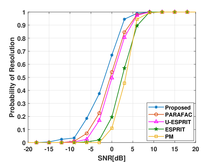
In our second example, the probability of resolution of two closely spaced targets with ${\varphi}_{k}=[20^{\circ},21^{\circ}]$ and ${\theta}_{k}=[15^{\circ},16^{\circ}]$ is analyzed. Two targets are considered to be resolved when $\left\|{{{\hat{\theta}}_{k}}-{\theta_{k}}}\right\|\leq\left\|{{\theta_{1}}-{\theta_{2}}}\right\|/2$ and $\left\|{{{\hat{\varphi}}_{k}}-{\varphi_{k}}}\right\|\leq\left\|{{\varphi_{1}}-{\varphi_{2}}}\right\|/2,\,k=1,2$. It can be seen from Fig. 2 that all methods exhibit resolution with probability 1 at high SNR, but the proposed method surpasses other methods as it has the lowest SNR threshold. The improved ability of resolving two closely spaced targets can be regarded as the advantage resulted from combining PARAFAC and ESPRIT. Moreover, the concatenation of tensors in (14) for different subarrays approximately doubles the number of samples. Thus, the proposed method achieves higher accuracy and better resolution for angle estimation.

A new tensor model for slow-time MIMO radar that enables improved joint DOD and DOA estimation for multiple targets has been proposed. This tensor can be regarded as an element-wise product of two tensors, where only one of them contains the angular parameters of interest. The model enables us to use PARAFAC decomposition with ESPRIT, and to address the problem of shortage of samples in Doppler domain for slow-time MIMO radar. As a result, the angle estimation performance has been improved as compared to the existing techniques.

To obtain (3), rewrite (2) as

Applying matched-filtering to ${{\bf{x}}_{nq}}$ in fast time, we have

where ${\eta_{nq}}\triangleq{\sigma_{k}^{2}{\beta_{n}}({\theta_{k}})\sum\limits_{m=1}^{M}{{\alpha_{m}}({\varphi_{k}}){e^{j2\pi({f_{k}}+{f_{m}})qT}}}}$ and ${{\bf{\bar{n}}}_{nq}}(t)$ is noise residue after matched-filtering. Since $\bf u$ is an LFM signal, the integral term ${{\bf F}(t)}=\int_{-\infty}^{\infty}{{\bf{u}}^{T}(t^{\prime}){\bf{u}}^{T}(t-t^{\prime})}dt^{\prime}$ is known to be approximately a $sinc$ function, and its peak indicates the range cell of the target.

Then, the concatenation of ${{\bf{\bar{x}}}_{nq}}$ in a single CPI with $Q$ pulses forms a $Q\times L$ matrix, i.e., $[{{\bf{\bar{x}}}^{T}_{n1}},{{\bf{\bar{x}}}^{T}_{n2}},\cdots,{{\bf{\bar{x}}}^{T}_{nQ}}]^{T}$. If fast Fourier transform (FFT) is applied to this matrix column-wisely, $M$ peaks with different Doppler frequencies can be found at the slice of target range cell. Each of the peaks corresponds to a unique transmit element as shown in the range-Doppler map shown in Fig. 3. The distance between two adjacent peaks in Doppler domain is determined by $\Delta f=f_{a}/M$. Owing to this Doppler frequency shifts for different transmitted waveforms, it is possible to distinguish each transmit channel at the receiver via filtering in Doppler domain.

For any $m$-th transmit element, the phase demodulation in Doppler domain is ${{\bf{\bar{x}}}_{nq,m}}={{\bf{\bar{x}}}_{nq}}{e^{-j2\pi{f_{m}}qT}}$. Equivalently

where ${\eta_{nq,m}}\triangleq{\sigma_{k}^{2}{\beta_{n}}({\theta_{k}}){\alpha_{m}}({\varphi_{k}}){e^{j2\pi{f_{k}}qT}}}$, ${\kappa_{nq,m}}\triangleq\sigma_{k}^{2}{\beta_{n}}({\theta_{k}})\sum\limits_{m^{\prime}\neq m}{{{\rm{\alpha}}_{m^{\prime}}}({\varphi_{k}}){e^{j2\pi({f_{m^{\prime}}}-{f_{m}}+{f_{k}})qT}}}$, and ${{\bf{\bar{z}}}_{nq,m}}(t)$ is the noise residue. After demodulation, each of $M$ transmit channels is shifted to baseband in Doppler domain (with a frequency of $f_{k}$). A reduced efficient Doppler range of $\left[{-\frac{{{f_{a}}}}{{2M}},\frac{{{f_{a}}}}{{2M}}}\right]$ is distributed to every transmit element (see Fig. 4 for more details). By applying lowpass filtering with cutoff frequency $\Delta f$, the second term ${\kappa_{nq,m}}{\bf{F}}{\rm{(t)}}$ in (21) can be omitted. Hence, the received signal from $m$-th transmit element to $n$-th receive element at $q$-th pulse can be expressed as

By range gating, the received signal is further expressed as

where $\bar{z}_{nq,m}$ is the slice of ${{\bf{\bar{z}}}_{nq,m}}(t)$ at the target range cell. Note that in order to avoid ambiguous Doppler returns, it is necessary to ensure that the highest Doppler frequency of interest $f_{k}$ is smaller than $\Delta f/2$. This implies that the DDMA technique achieves waveform diversity for slow-time MIMO radar at the cost of reduced Doppler frequency estimation range.

Another disadvantage is the decrease of the number of samples in Doppler domain. Recall ${\eta_{nq,m}}$, we have ${\eta_{nq,m}}=\sigma_{k}^{2}{\beta_{n}}({\theta_{k}}){\alpha_{m}}({\varphi_{k}}){e^{j2\pi\frac{{{f_{k}}}}{{{f_{a}}}}q}},\;q=1,2,\cdots,Q$. Clearly, this is a discrete signal with sampling rate $f_{a}$. The uniformly divided Doppler space then leads to the decline of sampling rate to $f_{a}/M$, i.e., ${{\eta}_{nq,m}}=\sigma_{k}^{2}{\beta_{n}}({\theta_{k}}){\alpha_{m}}({\varphi_{k}}){e^{j2\pi\left({\frac{{{f_{k}}}}{{{f_{a}}/M}}}\right)\frac{q}{M}}}$. Therefore,

where the number of efficient pulses is reduced to only $Q/M$. Here $Q/M$ is assumed to be an integer. Considering the noise term, the result in (3) is obtained.

References

- [1] E. Fishler, A. Haimovich et al., “MIMO radar: an idea whose time has come,” in Proc. IEEE Radar Conf., Apr. 2004, pp. 71–78.
- [2] V. S. Chernyak, “On the concept of MIMO radar,” in Proc. IEEE Radar Conf., May 2010, pp. 327–332.
- [3] J. Li and P. Stoica, “MIMO radar with colocated antennas,” IEEE Signal Process. Mag., vol. 24, no. 5, pp. 106–114, Sep. 2007.
- [4] A. M. Haimovich, R. S. Blum, and L. J. Cimini, “MIMO radar with widely separated antennas,” IEEE Signal Process. Mag., vol. 25, no. 1, pp. 116–129, Jan. 2008.
- [5] A. Hassanien and S. A. Vorobyov, “Phased-MIMO radar: A tradeoff between phased-array and MIMO radars,” IEEE Trans. Signal Process., vol. 58, no. 6, pp. 3137–3151, Jun. 2010.
- [6] E. Fishler, A. Haimovich et al., “Performance of MIMO radar systems: advantages of angular diversity,” in Proc. 38th Asilomar Conf. Signals, Syst. Comput., Pacific Grove, CA, Nov. 2004, pp. 305–309.
- [7] A. Hassanien and S. A. Vorobyov, “Transmit energy focusing for DOA estimation in MIMO radar with colocated antennas,” IEEE Trans. Signal Process., vol. 59, no. 6, pp. 2669–2682, Jun. 2011.
- [8] J. Li and P. Stoica, MIMO radar signal processing. New York: Wiley, 2009.
- [9] V. F. Mecca, D. Ramakrishnan, and J. L. Krolik, “MIMO radar space-time adaptive processing for multipath clutter mitigation,” in Proc. IEEE Workshop Sensor Array Multichannel Signal Processing, Jul. 2006, pp. 249–253.
- [10] D. W. Bliss, K. W. Forsythe et al., “GMTI MIMO radar,” in Proc. Int. Waveform Diversity Des. Conf., Feb. 2009, pp. 118–122.
- [11] J. M. Kantor and D. W. Bliss, “Clutter covariance matrices for GMTI MIMO radar,” in Proc. 44th Asilomar Conf. Signals, Syst., Comput., Nov. 2010, pp. 1821–1826.
- [12] X. Zhang, L. Xu, L. Xu, and D. Xu, “Direction of departure (dod) and direction of arrival (doa) estimation in MIMO radar with reduced-dimension MUSIC,” IEEE Commun. Lett., vol. 14, no. 12, pp. 1161–1163, Dec. 2010.
- [13] C. Duofang, C. Baixiao, and Q. Guodong, “Angle estimation using ESPRIT in MIMO radar,” Electron. Lett., vol. 44, no. 12, pp. 770–771, Jun. 2008.
- [14] G. Zheng, B. Chen, and M. Yang, “Unitary ESPRIT algorithm for bistatic MIMO radar,” Electron. Lett., vol. 48, no. 3, pp. 179–181, Feb. 2012.
- [15] Z. D. Zheng and J. Y. Zhang, “Fast method for multi-target localisation in bistatic MIMO radar,” Electron. Lett., vol. 47, no. 2, pp. 138–139, Jan. 2011.
- [16] N. D. Sidiropoulos, R. Bro, and G. B. Giannakis, “Parallel factor analysis in sensor array processing,” IEEE Trans. Signal Process., vol. 48, no. 8, pp. 2377–2388, Aug. 2000.
- [17] L. De Lathauwer, B. De Moor, and J. Vandewalle, “A multilinear singular value decomposition,” SIAM J. Matrix Anal. Appl., vol. 21, no. 4, pp. 1253–1278, 2000.
- [18] N. D. Sidiropoulos, L. De Lathauwer et al., “Tensor decomposition for signal processing and machine learning,” IEEE Trans. Signal Process., vol. 65, no. 13, pp. 3551–3582, Jul. 2017.
- [19] T. G. Kolda and B. W. Bader, “Tensor decompositions and applications,” SIAM Rev., vol. 51, no. 3, pp. 455–500, 2009.
- [20] D. Nion and N. D. Sidiropoulos, “Tensor algebra and multidimensional harmonic retrieval in signal processing for MIMO radar,” IEEE Trans. Signal Process., vol. 58, no. 11, pp. 5693–5705, Nov. 2010.
- [21] M. Cao, S. A. Vorobyov, and A. Hassanien, “Transmit array interpolation for DOA estimation via tensor decomposition in 2-D MIMO radar,” IEEE Trans. Signal Process., vol. 65, no. 19, pp. 5225–5239, Oct. 2017.
- [22] B. Xu, Y. Zhao, Z. Cheng, and H. Li, “A novel unitary PARAFAC method for DOD and DOA estimation in bistatic MIMO radar,” Signal Processing, vol. 138, pp. 273 – 279, 2017.
- [23] L. De Lathauwer and D. Nion, “Decompositions of a higher-order tensor in block terms—part III: Alternating least squares algorithms,” SIAM Rev., vol. 30, no. 3, pp. 1067–1083, 2008.
- [24] L. De Lathauwer, “A link between the canonical decomposition in multilinear algebra and simultaneous matrix diagonalization,” SIAM Rev., vol. 28, no. 3, pp. 642–666, 2006.
- [25] L. Sorber, M. Van Barel, and L. De Lathauwer, “Optimization-based algorithms for tensor decompositions: Canonical polyadic decomposition, decomposition in rank-(,,1) terms, and a new generalization,” SIAM Rev., vol. 23, no. 2, pp. 695–720, 2013.
- [26] X. Zhang, Z. Xu, L. Xu, and D. Xu, “Trilinear decomposition-based transmit angle and receive angle estimation for multiple-input multiple-output radar,” IET Radar, Sonar Navig., vol. 5, no. 6, pp. 626–631, Nov. 2011.
- [27] M. I. Skolnik, Radar handbook, 2nd ed. New York: McGraw-Hil, 1990.