SCALABILITY ANALYSIS OF DIRECT AND ITERATIVE SOLVERS USED TO MODEL CHARGING OF NON-INSULATED SUPERCONDUCTING PANCAKE SOLENOIDS

The discovery of high-temperature superconductors (HTS) [14, 26] opens a new chapter in both scientific and engineering fields for producing high-field superconducting magnets. Non-insulated superconductors in particular show great promise [15]. However, the numerical simulation of a non-insulated superconducting magnet is computationally expensive due to its highly non-linear electromagnetic behavior [35]. Though for simple geometries, the analytical solutions are possible to find under uniform external magnetic field [9, 32], time-dependent magnetic field simulation still remains a challenge to the scientific community even with the advanced computing facilities. This is because of (i) huge simulation domain as it includes air region along with the magnet that can produce multi-billions degrees of freedom (dofs) even taking advantage of symmetries (ii) complex magnet and conductor path geometry (iii) materials with widely disparate conductivity that can include an air region, $\sigma_{air}=1.0\hskip 2.84526ptS/m$, in direct contact with a superconducting region, $\sigma_{hts}=10^{15}\hskip 2.84526ptS/m$, producing a system matrix in a finite element discretization of the PDEs that can be highly ill-conditioned, and (iv) null-space of the $curl$-$curl$ operator in the governing Maxwell equations. Consider a sparse linear system

$\displaystyle A\boldsymbol{x}=\boldsymbol{b}\hskip 5.69054pt\text{with}\hskip 5.69054ptA\in\mathbb{R}^{N\times N},$

(1)

where $N$ is the order of the matrix $A$. The sparse direct solvers usually compute the $LU$ decomposition (or its variant) of the system matrix $A$ using its sparsity pattern in an efficient way so that it becomes easier to compute and store the factors. The direct solver inverts the system exactly, provides a very robust solution, and easy to use. For solving a typical PDE using a sparse direct solver, the computational cost grows as $O(N^{2})$ in 2D and $O(N^{7/3})$ in 3D, and memory requirement grows as $O(N\log N)$ in 2D and $O(N^{4/3})$ in 3D [5, 24]. Over the last few decades, due to the massive improvement in the sparse direct solvers, e.g., MUltifrontal Massively Parallel sparse direct Solver (MUMPS)¹¹ 1 http://mumps.enseeiht.fr/ [3, 4], PARDISO²² 2 https://www.pardiso-project.org/ [23], STRUMPACK [13, 34], SuperLU [25], or UMFPACK [11] have become popular among the researchers. Notwithstanding the advent of robust direct solvers, as the problem size and complexity increase, they require increasing computational time and computer memory and thus often fail to produce sufficiently resolved long range time-dependent solutions due to the limit of simulation time and memory constraint. Iterative solvers, e.g., CG [18], BiCGSTAB [43], MINRES [31], or GMRES [37] based on the Krylov subspace with appropriate preconditioners outperform [24] over the direct solver techniques in many complex problems. The computational cost can be of $O(N)$ or worse, and linear memory requirement $O(N)$ for the choice of the iterative solver and the preconditioner type [5]. The iterative solver does not solve the system exactly; it starts with an initial guess and continues to improve the solution in each iteration until the error/residual is less than a specified tolerance. The availability of good preconditioners is one of the main hurdles while using iterative solvers. Without good preconditioners, the issue of convergence arises, and the use of the iterative solver is not a good idea.

In this work, we explore numerical solution methods to simulate the charging behavior of non-insulated superconducting pancake solenoids. The mathematical model considers the magnetic field due to the current flow in complex 3D geometries in which a superconducting wire or coil is co-wound with a conducting metal, rather than an insulator, separating the turns. The superconductor is extremely thin with very high conductivity compared to the physical dimensions and conductivities of co-wound metals, and air. This introduces two extremely different time scales in the system which makes harder for the solvers to produce desire solutions. The objective of this research work is to find efficient solvers for the present work that can scale to multi-billions degrees of freedom anticipated in future applications. The finite element solutions for the fully discrete scheme are obtained by using an iterative solver combination (FGMRES-GMRES) with AMS preconditioner [19, 20] which is built in the hypre library [12], and the direct solver MUMPS. A scalability analysis for both direct and iterative solvers is presented. The scalability of the AMS preconditioner with conjugate-gradient (CG) method for low conductive materials is presented in [22]. To the best of our knowledge, the use of the robust FGMRES-GMRES solver with AMS preconditioner in simulating magnetic field with widely disparate material properties is new. All of the computational experiments presented in this paper are done in Petra-M [38].

The paper is organized as follows: In Section 2 we present mathematical modeling for the governing equations of magnetic field simulation. A brief description of the computational platform Petra-M is given in Section 3. In Section 4 we present the physical domains of the non-insulated superconducting pancake solenoids considered, provide a details description of the numerical experiment techniques, represent the scalability analysis for both direct and iterative solvers. Here the principal finding of this work is shown in both tabular and graphical forms, that the iterative solver with AMS preconditioner outperforms over the direct solver even with two extremely different time scales present in the system. In Section 5 we present conclusions and future research directions. Finally, in the appendix, we show the Biot-Savart magnetic field computation for the spiral coils.

In this paper, we consider a time varying magnetic field which is excited by imposing voltage to a body of conducting coil. The conducting coil is not strictly contained in the computational domain $\Omega$ as its two disjoint electric ports $\Gamma_{E}$ and $\Gamma_{J}$ touch the domain boundary $\partial\Omega$. We present the mathematical modeling of the time-dependent magnetic field following the frequency domain modeling in [33]. We neglect the displacement current density because we are concern with diffusive and not with wave timescales. Therefore, the Ampere’s law in differential form [7]:

$\displaystyle\nabla\times\boldsymbol{H}={\bf{J}}=\sigma{\bf E},$

(2)

where $\boldsymbol{H}$ the magnetic field strength, ${\bf{J}}$ the current density, ${\bf E}$ the electric field strength, and $\sigma$ the conductivity. For simplicity we consider $\sigma$ as a positive constant in this paper rather than a tensor. Dividing both sides by $\sigma$, and taking curl operator

$\displaystyle\nabla\times\frac{1}{\sigma}\nabla\times\boldsymbol{H}=\nabla\times{\bf E}.$

(3)

Faraday’s law of induction:

$\displaystyle\nabla\times{\bf E}=-\frac{\partial\boldsymbol{B}}{\partial t}=-\mu_{0}\frac{\partial\boldsymbol{H}}{\partial t},$

(4)

for the magnetic flux density $\boldsymbol{B}=\mu_{0}\boldsymbol{H}$, where $\mu_{0}$ is a material independent parameter called the permeability constant. The equation (4) ensures that if the initial magnetic field strength is divergence free then $\nabla\cdot\boldsymbol{H}=0$ holds for all time. We assume $\Gamma_{E}$ and $\Gamma_{J}$ are perfect conductors, and thus the tangential component of the electric field vanishes there. Thus, we consider the following no-flux boundary conditions [8, 33]

	$\displaystyle{\bf E}\times\hat{\textbf{{n}}}=\frac{1}{\sigma}\nabla\times\boldsymbol{H}\times\hat{\textbf{{n}}}$	$\displaystyle=\textbf{0},\hskip 5.69054pt\text{in}\hskip 5.69054pt\Gamma_{E}\cup\Gamma_{J}\times(0,T],$		(5)
	$\displaystyle\mu_{0}\boldsymbol{H}\cdot\hat{\textbf{{n}}}$	$\displaystyle=0,\hskip 5.69054pt\text{in}\hskip 5.69054pt\partial\Omega\times(0,T],$		(6)

where $\hat{\textbf{{n}}}$ is the outward unit normal vector to the boundary, and $T$ the simulation time. We apply a fixed non-zero voltage $V$ at $\Gamma_{J}$ and zero voltage at $\Gamma_{E}$, this potential difference drives the current to pass along the coil. Taking the dot product of $\hat{\textbf{{n}}}$ on both sides of (4) and using (6) we have $\nabla\cdot({\bf E}\times\hat{\textbf{{n}}})=0\hskip 5.69054pt\text{on}\hskip 5.69054pt\partial\Omega.$ Assuming the boundary $\partial\Omega$ a simply-connected surface, there exists a surface potential $v$ such that

$\displaystyle{\bf E}\times\hat{\textbf{{n}}}=\frac{1}{\sigma}\nabla\times\boldsymbol{H}\times\hat{\textbf{{n}}}=\nabla v\times\hat{\textbf{{n}}}\hskip 5.69054pt\text{on}\hskip 5.69054pt\partial\Omega,$

(7)

where $v_{|_{\Gamma_{J}}}=V$ is a non-zero constant and $v_{|_{\Gamma_{E}}}=0$. Combining the equations (3)-(4), and (7) we have the following time-dependent governing equations for the magnetic field simulation of the voltage excitation problem

	$\displaystyle\frac{\partial\boldsymbol{H}}{\partial t}+\frac{1}{\mu_{0}}\nabla\times\frac{1}{\sigma}\nabla\times\boldsymbol{H}$	$\displaystyle=\textbf{0},\hskip 28.45274pt\forall(x,t)\in\Omega\times(0,T],$		(8)
	$\displaystyle{\color[rgb]{0,0,0}\frac{1}{\sigma}\nabla\times\boldsymbol{H}\times\hat{\textbf{{n}}}}$	$\displaystyle={\color[rgb]{0,0,0}\nabla v\times\hat{\textbf{{n}}}},\hskip 2.84526pt\forall(x,t)\in\partial\Omega\times(0,T],$		(9)
	$\displaystyle\boldsymbol{H}(x,0)$	$\displaystyle=\textbf{0},\hskip 31.29802pt\forall x\in\Omega,$		(10)

where $v_{|_{\Gamma_{J}}}=V$ and $v_{|_{\Gamma_{E}}}=0$.

We note that this is a diffusion equation for the magnetic field with characteristic time given by $t_{\rm d}=\mu_{0}\sigma l^{2}$, where $l$ is a characteristic length scale. In the simulations shown in the following sections, the time is normalized by this diffusion time, where $l=1.14m$ and $\sigma=2\times 10^{6}S/m$ are used. Additionally, the magnetic fields are normalized by the field produced by a single turn coil with same current ($I=$1000A), defined as $B_{0}:=\mu_{0}I/l$.

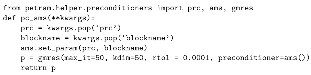
The time-dependent equations (8)-(10) was discretized fully by the backward-Euler timestepping scheme and solved on the Petra-M [38] finite element analysis platform. This open source platform allows for constructing a geometry, creating a mesh, assembling and solving the finite element linear system, and solving and visualizing the results using a user friendly graphical interface (GUI). Petra-M uses various open source software. In particular, it uses MFEM modular finite element library [1] for the FEM linear system assembly. The weakform PDE interface in Petra-M allows for defining a mixed form PDE system we solved in this paper by choosing form integrators available in the MFEM library from menus. Petra-M combines GUIs with the python scripting, allowing for rapidly developing the simulation model with very little coding effort. For example, the inner solver with pre-conditioner is defined in the code segment is given Fig. 1. Then, the outer solver is configured to use this inner solver using GUI. All simulations are done on the ‘Engaging’ cluster computer at the Massachusetts Institute of Technology, in which one node consists of 32 cores and 512 GB RAM memory.

For our simulations, we consider four different geometries for the charging pancake solenoids: One turn single pancake (T-1), ten turns double pancakes (T-10) with each pancake has five turns, twenty turns double pancakes (T-20) with each pancake has ten turns, and thirty turns double pancakes (T-30) with each pancake has fifteen turns. The cross-section of the HTS spiral coils are rectangular. The thickness and height of the HTS coil are $0.16cm$ and $0.3cm$, respectively for all of the four models. In each of the geometry, the HTS coil is co-wound with copper with a rectangular cross-section, which is then co-wound with stainless steel. The copper and stainless steel co-wounds help not to arise numerical issues as they prevent the superconducting coil from directly touching the air. The copper co-wound spiral coil preserves the spiral pattern of the HTS coil, keeping the uniform gap between turn to turn. A sufficiently large air domain is considered surrounding the stainless steel body so that the magnetic field lines do not go beyond it. Finally the terminals of the copper co-wound HTS coil are extended to the air boundary by solid copper rectangular bars. The two copper terminals are extended to the boundary so that external voltage can be applied to one of them, and the voltage drives the current to flow along the spiral coil and the magnetic field is produced. Thus, in this work, we consider forced voltage excitation coil [27, 33], and the voltage is adjusted to have the same current for all four models [10].

The physical properties of the different models are described below:

Numerical solutions of complex PDEs are often one of the most challenging tasks, which involve finding solutions of systems of linear equations with multi-billions degrees of freedom. In this paper, we have presented a voltage excited magnetic field formulation for the charging simulation of non-insulated superconducting pancake solenoids. The numerical difficulty for the simulation of the problem arises from the fact that the HTS coil is very thin but with excessively high conductivity whereas its surrounding materials have the opposite properties.

In this paper, we have explored an iterative solver for Maxwell’s equation simulation, which is a combination FGMRES and GMRES solver with a parallel AMS Solver preconditioner. We have investigated the scalability performance of the direct solver, MUMPS, and the iterative solver, FGMRES-GMRES with AMS preconditioner, on 1, 10, 20, and 30 turns pancake solenoids. The direct solver is efficacious for problems with fewer degrees of freedom and provides an additional advantage when the conductivity of the diffusion equation is independent of time. Since in this case, the system matrix remains same for all time step but the right hand side vector changes and the direct solver factorizes the system matrix only once and repeatedly use them for the further timesteps. On the other hand, the iterative solver is faster, uses less memory, and scale better than the direct solver, especially to the problem that has complex geometry and/or higher degrees of freedom. This iterative solver along with the AMS preconditioner can successfully solve the problem of size with at least 48 million degrees of freedom.

As a benchmark, we have computed the Biot-Savart fields and compared them with the FEM results, and found excellent agreement. It is observed that if we increase the number of turns in a charging solenoid, the charging time of the model and the computational time of the iterative solver both increase. Finally, we have also found that as the conductivity of the superconductor increases the problem becomes harder and the iterative solver needs longer time to converge.

We believe the most important future research avenue would be the incorporation of quench analysis [6] in our mathematical model and explore the charging behavior of non-insulated superconducting pancake solenoids. We will use the proposed efficient solver, FGMRES-GMRES, for problems with large degrees of freedom, and will continue to investigate further for a better preconditioner.

Apart from the voltage excitation problem, we plan to investigate a current intensity excitation modeling [33] and explore the charging behavior ramping up the current slowly. In a current intensity excitation problem, the voltage remains an unknown.

Instead of $\boldsymbol{H}$-formulation, we plan to investigate the eddy current simulation on a multiply connected region based on $\boldsymbol{H}-\Phi$ field formulation following the work in [41]. The magnetic field $\boldsymbol{H}$ will be computed using the iterative solver in the conducting region and the multi-valued magnetic scalar potential $\Phi$ will be the solution of a diffusion BVP in the non-conduction region. Finally, both solutions will be assembled together using the appropriate tangential continuity condition across the interfaces between different tetrahedral elements. This approach will potentially reduce the cost of computing the magnetic field in the air domain.

We plan to explore the stability and error estimate analysis for the fully discrete scheme used in this paper following the works in [2, 17]. The study of ensemble magnetic field calculations [28] with the advantage of block linear solver can also be a new research avenue. We also want to explore the reduced order modeling of the magnetic field simulation in a non-insulated superconducting pancake solenoids following the analysis and experiments given in [29].

Acknowledgment. The work was supported by Commonwealth Fusion Systems grant RPP002. We thank Dan Brunner for his constructive comments and suggestions, which significantly improved the quality of the manuscript.

References

- [1] MFEM: Modular finite element methods library. https://mfem.org/.
- [2] M. Akbas, S. Kaya, M. Mohebujjaman, and L. Rebholz. Numerical analysis and testing of a fully discrete, decoupled penalty-projection algorithm for mhd in elsässer variable. Int. J. Numer. Anal. Model, 13(1):90–113, 2016.
- [3] P. R. Amestoy, I. S. Duff, and J. L′Excellent. Multifrontal parallel distributed symmetric and unsymmetric solvers. Computer methods in applied mechanics and engineering, 184(2-4):501–520, 2000.
- [4] P. R. Amestoy, I. S. Duff, J. L′Excellent, and J. Koster. MUMPS: A general purpose distributed memory sparse solver. Sørevik T., Manne F., Gebremedhin A.H., Moe R. (eds) Applied Parallel Computing. New Paradigms for HPC in Industry and Academia. PARA 2000. Lecture Notes in Computer Science, 1947:121–130, 2000.
- [5] W. Bangerth. Finite element methods in scientific computing, Lecture 34: What solver to use. https://www.math.colostate.edu/~bangerth/videos/676/slides.34.pdf.
- [6] K. R. Bhattarai, K. Kim, K. Kim, K. Radcliff, X. Hu, C. Im, T. Painter, I. Dixon, D. Larbalestier, S. Lee, and S. Hahn. Understanding quench in no-insulation (ni) rebco magnets through experiments and simulations. Superconductor Science and Technology, 33(3):035002, 2020.
- [7] O. Bíró. Edge element formulations of eddy current problems. Computer methods in applied mechanics and engineering, 169(3-4):391–405, 1999.
- [8] A. Bossavit. Most general ‘non-local’ boundary conditions for the maxwell equation in a bounded region. COMPEL, 19(2):239–245, 2000.
- [9] E. H. Brandt. Superconductors of finite thickness in a perpendicular magnetic field: Strips and slabs. Physical Review B, 54(6):4246–4264, 1996.
- [10] S. By, J. V. Rispoli, S. Cheshkov, I. Dimitrov, J. Cui, S. Seiler, S. Goudreau, C. Malloy, S. M. Wright, and M. P. McDougall. A 16-channel receive, forced current excitation dual-transmit coil for breast imaging at 7T. PloS one, 9(11), 2014.
- [11] T. A. Davis. Algorithm 832: UMFPACK v4.3—an unsymmetric-pattern multifrontal method. ACM Transactions on Mathematical Software (TOMS), 30(2):196–199, 2004.
- [12] R. D. Falgout and U. M. Yang. hypre: A library of high performance preconditioners. International Conference on Computational Science, pages 632–641, 2002.
- [13] P. Ghysels, X. S. Li, F. Rouet, S. Williams, and A. Napov. An efficient multicore implementation of a novel hss-structured multifrontal solver using randomized sampling. SIAM Journal on Scientific Computing, 38(5):S358–S384, 2016.
- [14] D. M. Ginsberg. Physical properties of high temperature superconductors III, volume 3. World Scientific, 1992.
- [15] S. Hahn, D. K. Park, J. Bascunan, and Y. Iwasa. HTS pancake coils without turn-to-turn insulation. IEEE transactions on applied superconductivity, 21(3):1592–1595, 2010.
- [16] B. He, C. Lu, N. Chen, D. Lin, and P. Zhou. An efficient parallel computing method for the steady-state analysis of electric machines using the woodbury formula. IEEE Transactions on Magnetics, 56(2):1–4, 2020.
- [17] T. Heister, M. Mohebujjaman, and L. G. Rebholz. Decoupled, unconditionally stable, higher order discretizations for mhd flow simulation. Journal of Scientific Computing, 71(1):21–43, 2017.
- [18] M. R. Hestenes and E. Stiefel. Methods of conjugate gradients for solving linear systems. Journal of research of the National Bureau of Standards, 49(6):409–436, 1952.
- [19] R. Hiptmair, G. Widmer, and J. Zou. Auxiliary space preconditioning in . Numerische Mathematik, 103(3):435–459, 2006.
- [20] R. Hiptmair and J. Xu. Auxiliary space preconditioning for edge elements. IEEE Transactions on Magnetics, 44(6):938–941, 2008.
- [21] Z. Huo, G. Mei, G. Casolla, and F. Giampaolo. Designing an efficient parallel spectral clustering algorithm on multi-core processors in julia. Journal of Parallel and Distributed Computing, 2020.
- [22] T. V. Kolev and P. S. Vassilevski. Parallel auxiliary space AMG for H (curl) problems. Journal of Computational Mathematics, pages 604–623, 2009.
- [23] A. Kuzmin, M. Luisier, and O. Schenk. Fast methods for computing selected elements of the green’s function in massively parallel nanoelectronic device simulations. In European Conference on Parallel Processing, pages 533–544. Springer, 2013.
- [24] U. Langer and M. Neumüller. Direct and iterative solvers. In Computational Acoustics, pages 205–251. Springer, 2018.
- [25] X. S. Li, J. Demmel, J. Gilbert, L. Grigori, and M. Shao. SuperLU. Encyclopedia of Parallel Computing, pages 1955–1962, 2011.
- [26] D. Liu, H. Yong, and Y. Zhou. Analysis of charging and sudden-discharging characteristics of no-insulation rebco coil using an electromagnetic coupling model. AIP Advances, 7(11):115104, 2017.
- [27] S. Meng, B. Zhu, Z. Zhuang, X. Chen, and C. Tang. Effect of excitation coil voltage on TiAlSiN coating on 42crmo steel surface. Materials Research Express, 7(5):056519, 2020.
- [28] M. Mohebujjaman and L. G. Rebholz. An efficient algorithm for computation of mhd flow ensembles. Computational Methods in Applied Mathematics, 17(1):121–137, 2017.
- [29] M. Mohebujjaman, L. G. Rebholz, X. Xie, and T. Iliescu. Energy balance and mass conservation in reduced order models of fluid flows. Journal of Computational Physics, 346:262–277, 2017.
- [30] K. Ono, T. Kato, S. Ohshima, and T. Nanri. Scalable direct-iterative hybrid solver for sparse matrices on multi-core and vector architectures. In Proceedings of the International Conference on High Performance Computing in Asia-Pacific Region, pages 11–21, 2020.
- [31] C. C. Paige and M. A. Saunders. Solution of sparse indefinite systems of linear equations. SIAM journal on numerical analysis, 12(4):617–629, 1975.
- [32] L. Prigozhin. The bean model in superconductivity: Variational formulation and numerical solution. Journal of Computational Physics, 129(1):190–200, 1996.
- [33] A. A. Rodríguez and A. Valli. Eddy current approximation of Maxwell equations: Theory, algorithms and applications, volume 4. Springer Science & Business Media, 2010.
- [34] F. Rouet, X. S. Li, P. Ghysels, and A. Napov. A distributed-memory package for dense hierarchically semi-separable matrix computations using randomization. ACM Transactions on Mathematical Software (TOMS), 42(4):1–35, 2016.
- [35] D. Ruiz-Alonso, T. Coombs, and A. M. Campbell. Computer modelling of high-temperature superconductors using an A–V formulation. Superconductor Science and Technology, 17(5):S305, 2004.
- [36] Y. Saad. A flexible inner-outer preconditioned gmres algorithm. SIAM Journal on Scientific Computing, 14(2):461–469, 1993.
- [37] Y. Saad and M. H. Schultz. GMRES: A generalized minimal residual algorithm for solving nonsymmetric linear systems. SIAM Journal on scientific and statistical computing, 7(3):856–869, 1986.
- [38] S. Shiraiwa, J. C. Wright, P. T. Bonoli, T. Kolev, and M. Stowell. RF wave simulation for cold edge plasmas using the MFEM library. EPJ Web of Conferences, 157(03048), 2017.
- [39] H. Shoukourian, T. Wilde, A. Auweter, and A. Bode. Predicting the energy and power consumption of strong and weak scaling hpc applications. Supercomputing frontiers and innovations, 1(2):20–41, 2014.
- [40] V. Simoncini and D. B. Szyld. Flexible inner-outer krylov subspace methods. SIAM Journal on Numerical Analysis, 40(6):2219–2239, 2003.
- [41] J. Smajic, M. K. Bucher, C. Jäger, and R. Christen. Treatment of multiply connected domains in time-domain discontinuous galerkin eddy current analysis. IEEE Transactions on Magnetics, 55(6):1–4, 2019.
- [42] X. Sun and D. T. Rover. Scalability of parallel algorithm-machine combinations. IEEE Transactions on parallel and Distributed Systems, 5(6):599–613, 1994.
- [43] H. A. Van der Vorst. Bi-CGSTAB: A fast and smoothly converging variant of Bi-CG for the solution of nonsymmetric linear systems. SIAM Journal on scientific and Statistical Computing, 13(2):631–644, 1992.