Pulsar radio emission mechanism I : On the amplification of Langmuir waves in the linear regime2015Pulsar radio emission mechanism I : On the amplification of Langmuir waves in the linear regime–References
Abstract
Observations suggest that in normal period radio pulsars, coherent curvature radiation is excited within 10 of the light cylinder. The coherence is attributed to Langmuir mode instability in a relativistically streaming one-dimensional plasma flow along the open magnetic field lines. In this work, we use a hot plasma treatment to solve the hydrodynamic dispersion relation of Langmuir mode for realistic pulsar parameters. The solution involves three scenarios of two-stream instability viz., driven by high energy beams, due to longitudinal drift that leads to a separation of electron-positron distribution functions in the secondary plasma and due to cloud-cloud interaction causing spatial overlap of two successive secondary plasma clouds. We find that sufficient amplification can be obtained only for the latter two scenarios. Our analysis shows that longitudinal drift is characterized by high growth rates only for certain multi-polar surface field geometry. For these configurations, very high growth rates are obtained starting from a few tens of km from the neutron star surface, which then falls monotonically with increasing distance. For cloud-cloud overlap, growth rates become high starting only after a few hundred km from the surface, which first increases and then decreases with increasing distance. A spatial window of up to around a 1000 km above the neutron star surface has been found where large amplitude Langmuir waves can be excited while the pair plasma is dense enough to account for high brightness temperature.
Keywords:
pulsars – radiation mechanism – relativistic plasma – Langmuir mode1 Introduction
Observations of radio emission from normal period pulsars (with periods longer than 0.1 seconds) suggest that: a) The radio emission has exceedingly high brightness temperature K, which is at least 12 orders of magnitude higher than the incoherent synchrotron limit of K (see Kellermann & Pauliny-Toth 1969 ). This necessarily requires a coherent radio emission mechanism (e.g. Ginzburg et al. 1969; Ginzburg & Zhelezniakov 1975; Cordes 1979; Melrose 1993; Mitra 2017) ; b) The radio emission is highly polarized, which is consistent with coherent curvature radiation ( hereafter CCR ) (e.g. Mitra et al. 2009; Melikidze et al. 2014) ; c) The radio emission detaches from the pulsar magnetosphere a few hundred km away from the surface (e.g. Rankin 1993; Mitra 2017).
These observations require plasma processes where stable charge bunches can form and excite CCR in relativistically streaming pair plasma, which can eventually escape from the plasma to reach the observer (see Melikidze et al. 2014; Gil et al. 2004; Mitra et al. 2009). For a general non-zero angle between the propagation vector and the ambient magnetic field, the pulsar pair plasma consists of two eigen-modes viz., the purely transverse X-mode and the quasi-transverse O-mode (see Arons & Barnard 1986). The quasi-transverse O-mode has a sub-Lumininal Alfven branch and super-Luminal LO branch. A number of works show that cyclotron instabilities of the X and O modes can be excited close to the light-cylinder (see for e.g. Kazbegi et al. 1991; Lyutikov 1999). However, several works have shown that close to neutron star surface, where the radio emission originates, the excitation of the Alfvén branch is inefficient(e.g. Lominadze et al. 1986; Kazbegi et al. 1991 ; Lyutikov 2000). For the special case when the angle between the propagation vector and the ambient magnetic field is zero, the O-mode becomes purely longitudinal and is referred to as the Langmuir mode (see fig. 2 of Arons & Barnard 1986). It has been shown in several studies (e.g. Usov 2002) that closer to the neutron star surface this longitudional Langmuir mode can become unstable. Langmuir mode instability is a popular candidate for these CCR charge bunches. Theoretically, a combination of linear and non-linear plasma theory is needed to form stable charge bunch (see Melikidze et al. 2000). The linear part of the theory involves development of two stream instability in the plasma that leads to the growth of the amplitude of the longitudinal and electrostatic Langmuir wave mode. While the oscillating electric field of the Langmuir mode can form longitudinal concentrations of charges, it is well known that such linear Langmuir bunches are not capable of radiating coherently (see e.g. Lominadze et al. 1986; Melikidze et al. 2000). Analytical studies show that under certain approximations stable bunches viz. relativistic Langmuir charge soliton can form when non-linear effects are taken into account (see Pataraia & Melikidze 1980; Melikidze et al. 2000). Recent numerical analysis have also found such stable charge bunches, when all non-linear interactions are properly taken into account (see Lakoba et al. 2018). However there are several gaps in the theory that remains to be addressed. The non-linear theory requires a priori very large amplitude for the electrostatic waves. The crucial question of quantitative estimates of linear growth rates of Langmuir waves for realistic pulsar plasma parameters, and if the growth rate is sufficient to drive the system beyond the linear regime requires thorough investigation.
The radio emission is excited in relativistically streaming pulsar plasma that consists of a dense secondary positron-electron () pair plasma, a tenuous high energy primary positron or electron () beam and a tenuous high energy ion beam. The growth of Langmuir instability requires a two-stream condition to be established in this plasma. Some early works on Langmuir mode in pulsar plasma in fact concluded that Langmuir mode cannot become unstable (e.g. Suvorov & Chugunov 1975 ). However Lominadze & Mikhailovskiǐ 1979, discussed that in relativistic plasma, particles close to the velocity of light can be in resonance with the Langmuir mode. The authors also discussed two regimes of growth viz., the kinetic and the hydrodynamic regime. There are three ways (referred to as case C1, C2, C3 hereafter) by which the two-stream instability can develop in this flow: first for C1 between the high energy beams and secondary plasma system, second for C2 between the electrons and positrons in the secondary plasma itself due to longitudinal drift, and third for C3 between the overlapping fast and slow particles overlap of successive secondary plasma clouds due to intermittent discharges at the polar gap.
Previous studies of the growth of Langmuir wave in pulsar plasma for the three aforementioned cases of two-stream instability can be briefly summarized as follows:
C1: Initial studies of pulsar radio emission mechanism (e.g. Ruderman & Sutherland 1975 hereafter RS75) appealed to a two-stream instability driven by high energy cold beam. Subsequent works(e.g. Benford & Buschauer 1977) found very small growth rates for such cold beam. Egorenkov et al. 1983 presented a hot plasma treatment of the high energy beam and showed that kinetic regime is suppressed and only the hydrodynamic regime survives. Gedalin et al. 2002 explored beam-driven hydrodynamic instability of a low frequency longitudinal beam mode rather than the high-frequency Langmuir mode. Most of the subsequent works (see Lyutikov 1999; Melrose & Gedalin 1999; Rafat et al. 2019) have focussed on this beam and found the growth rates to be negligible.
C2: The study by Cheng & Ruderman 1977 showed that as the secondary pair plasma moves along the curved magnetic field line, longitudinal drift causes the electron and positron distribution function to separate. This can lead to two-stream instability in the secondary plasma. However, they did not consider a hot plasma treatment of the secondary plasma and obtained order of magnitude estimates of growth rate using simple assumptions. Asseo & Melikidze 1998 revisited the problem where they presented a hot plasma treatment of the shifted electron-positron distribution function within the secondary plasma cloud.
C3: Usov 1987 showed that in non-stationary plasma flow models, slow and fast moving particles of two successive plasma clouds can overlap within a few hundred km from the surface leading to the development of a two-stream instability in the overlapping region. Ursov & Usov 1988 revisited the problem and tried to estimate growth rates by approximating the distribution function of the fast and slow particles in the overlapping region by delta-function. AM98 extended and presented a more realistic analytical way of constructing the form of the hot plasma distribution function in the overlapping region.
The aforementioned studies suggest that large amplitude Langmuir wave cannot exist due to beam in C1. AM98 showed that two-stream instability in C2 and C3 can result in high growth rates of Langmuir wave. They also found that the growth rate for C3 to be significantly larger than C2. Thus AM98 provided the necessary justification, that in principle large amplitude Langmuir waves can be triggered for both C2 and C3.
However AM98 obtained growth rates in the hydrodynamic regime for C2 and C3 using many simplifying assumptions. For example, they assumed the surface magnetic field to be dipolar while observations suggest the existence of a strong multipolar magnetic field at the surface. Also, they estimated growth rates as a function of the distance from the neutron star, using coarse spatial ( and temporal ) resolution. In their numerical scheme, AM98 did not obtain the complete solution of the dispersion relation at a given height and estimated growth rates only for some representative wave numbers. The coarse resolution in their analysis can wash away many important features of the evolution of the growth rate as a function of the distance from the neutron star. Hence it is necessary to undertake an updated study of AM98 where these shortcomings should be addressed appropriately. This is the primary focus of this work. Further keeping in view that a tenous high energy beam of ions can exist, we study the effect of the same on Langmuir mode instability in C1 and compare it with the beam.
It must be noted that the amplification of the Langmuir wave for a given frequency depends on the gain ‘G’ which is a product of the growth rate () and the time available for growth () as the amplitude is . If time is small, even with a high , the amplification factor will be small and one cannot use these waves to participate in the coherent emission mechanism. In this work, we go beyond just the estimation of growth rate and present a method that employs the complete bandwidth of the growing waves to estimate and thereby the maximum gain possible for a given frequency. We present an exhaustive treatment of Langmuir mode instability for C1, C2 and C3 to examine the existence of large amplitude Langmuir waves in the pulsar radio emission region. The outline of the paper is as follows: In sections 2 we discuss physical constraints for the hot plasma description and models of plasma flow. In sections 3 and 4 we describe the analysis method for the linear Langmuir instability and study the growth rates and gain factors for these cases. In sections 5 and 6 we discuss the results and state our conclusions.
2 Inputs to the pulsar plasma parameters
2.1 Constraints from radio emission height
A number of studies : Blaskiewicz et al. 1991, von Hoensbroech & Xilouris 1997 , Mitra & Li 2004 , Mitra & Rankin 2011 , Weltevrede & Johnston 2008 has consistently found the emission region to be below 10 of LC across pulsar period (see fig. 3 of Mitra 2017). As discussed by Mitra & Li 2004, the various methods employed to find radio emission heights can be affected due to measurement as well as systematic errors, however for normal pulsars average estimates of a few hundred kilometers above the neutron star surface is considered reasonable. Specific studies (e.g. Mitra & Rankin 2002) also, focus on estimating the range of emission heights as a function of frequency, and it is found that a certain radius to frequency mapping exists in pulsars where progressively higher frequencies arise closer and closer to the neutron star surface. These studies reveal that the broad-band pulsar emission range from about few ten to hundred km at the highest frequency GHz and to several hundred km at the lowest frequency MHz. Kazbegi et al. 1991 showed that cyclotron resonances can be excited only near the light cylinder. At the radio emission heights all cyclotron resonances are suppressed and only the Cherenkóv resonance condition can operate.
2.2 Signature of Coherent Curvature Radiation
Several lines of evidence (see Lai et al. 2001; Johnston et al. 2005; Rankin 2007; Noutsos et al. 2012; Noutsos et al. 2013; Force et al. 2015) have revealed that the polarization of the emergent pulsar radiation are directed either perpendicular or parallel to the magnetic field line plane. These polarization modes are commonly referred to as the extraordinary and Ordinary mode respectively which are defined with their electric field vector being perpendicular and parallel to the magnetic field plane respectively. The eigenmodes of the pulsar plasma viz., the X-mode and the O-mode is perpendicular and parallel to the plane, where is the ambient magnetic field and is the propagation vector of the wave. If the underlying excitation mechanism is due to CCR, then these two planes need to be co-incident. For any other form of excitation, these two planes can maintain arbitrary orientation to each other. This implies that the polarization of emergent radiation carries information about the underlying excitation mechanism. This idea was applied by Mitra et al. 2009 to a sample of nearly 100 linearly polarized single pulses which established CCR as the underlying emission mechanism.
2.3 Multi-polar surface magnetic fields and particle flows
It is well known (see e.g. Mitra & Li 2004) that at a few hundred kilometers above the neutron star surface, from regions where the radio emission originates, the underlying magnetic field structure is dipolar. However, in recent years there are several pieces of evidence for the presence of surface multipolar fields. For example Gil & Mitra 2001 and Mitra et al. 2020 suggested that the radio-loud nature of the extremal long period 8.5 s pulsar J2144-3933 (Young et al. 1999) can only be explained if surface magnetic fields have a radius of curvature cm at the surface, which is only possible due to presence of strong multipolar surface magnetic field. The X-ray observations have also confirmed the presence of multipolar fields on the surface (see e.g. Arumugasamy & Mitra 2019).
The presence of multipolar surface magnetic field significantly affects the description of the plasma. At the polar cap magnetically induced pair creation processes are triggered. The presence of multipolar surface magnetic field decreases the radius of curvature at the surface thereby increasing the efficiency of the pair creation process. As a result the number density of the pair plasma exceeds the co-rotational value by a multiplicity factor . Observations of PWNe has revealed (see de Jager 2007 ; Blasi & Amato 2011 ). To get this high value of estimations show that to get multi-polar fields are required (see Medin & Lai 2010 ; Szary et al. 2015 ; Timokhin & Harding 2019) whereas for purely dipolar fields is about the order of a few tens to hundred (see Hibschman & Arons 2001; Arendt & Eilek 2002)
2.3.1 Need for multipolar surface magnetic field for CCR
The limiting brightness temperature for incoherent curvature radiation is K (see Melrose 1978). In the Rayleigh-Jeans regime, the brightness temperature is proportional to power. CCR is an ‘’ process meaning if ‘’ particles are involved, the power is boosted by a factor ‘’ compared to what would be achieved if the charged particles were emitting independently (or incoherently). The number of particles participating in CCR to explain the observed high brightness temperature is given by . Radio emission from pulsars are received from MHz to GHz. The length of the bunch should satisfy the constraint cm for coherence to be maintained for all frequencies. Assuming cm, the corresponding number density required cm-3. At an emission height of , the Goldreich-Julian value is given by secGauss cm-3 (see Goldreich & Julian 1969). Thus, CCR requires number density in excess of the Goldreich-Julian value by a factor of .
2.3.2 Description of particle flow and secondary plasma distribution functions
The models of plasma flow can be divided into two classes: a) The steady flow model (also known as SCLF model) given by Arons & Scharlemann 1979 where when condition above the polar cap is such that (here is the pulsar rotational frequency), the electrons can be easily pulled out from the star and a stationary flow of electron beam-plasma can be maintained and; b) The non-stationary spark discharge model (also referred to Inner acceleration gap model or the pure vacuum gap model) by RS75 for pulsars with giving rise to an intermittent plasma flow due to sparking discharges at the polar gap. In both these models the beam-plasma system is established.
The vacuum gap model of RS75 is more successful in explaining pulsar radio observations like sub-pulse drift phenomenon, however the original model required certain modifications. Gil et al. 2003 noticed that the sub-pulse drift rates and the temperature of the thermal X-ray emitting polar cap are both lower than that predicted by the pure vacuum gap model of RS75. They suggested that the pure vacuum gap is untenable and must be partially screened such that the potential is across the gap is replaced by where is the screening factor. For a pulsar of period 1 second and dipolar magnetic strength of gauss, the maximum potential drop available in vacuum is volts. The authors constrained , which gives the Lorentz factor of the high energy primary beams of and ions to be given by and respectively. Assuming CCR we can find an order of magnitude estimate of the bulk Lorentz factor of the secondary pair plasma. Most of the power in CCR for charge bunch with Lorentz factor is concentrated near the critical frequency , (see Jackson 1962, where is the velocity of light). Assuming observing frequency GHz to be close to the critical frequency at where cm, we have .
For our work we assume the distribution functions of all the species to be relativistically streaming gaussians. For secondary plasma, the mean and the width are assumed to be and respectively. Note that the two stream-condition can be established in non-stationary flow by all three cases of C1, C2 and C3 whereas for stationary flow only the cases C1 and C2.
To summarize CCR needs to be excited by large amplitude Langmuir waves in a hot relativistically streaming dense secondary pair plasma . At the radio emission heights, the wave-particle interaction is mediated by the Cherenkóv resonance condition. In subsequent sections we address how large amplitude Langmuir waves can be triggered for the three cases, C1,C2, C3 of two-stream instability discussed earlier.
3 Analysis of Langmuir instability
In the following subsections, we establish the methodology for studying Langmuir instability. To do this we define a threshold gain for a wave of a particular frequency that can be used as a proxy for the breakdown of the linear theory. This, in turn, is achieved by solving the complex frequencies using the appropriate dispersion relation. For this analysis, the following aspects need to be considered.
3.1 The Dispersion relation in the observer frame of reference
The dispersion relation of the Langmuir mode for a strictly one-dimensional relativistic flow in the observer frame of reference is given by (see section 4 of AM98)
| (1) |
where . Here , , , and is the number density, charge, mass, dimensionless momenta and the equilibrium distribution function of the -th species in the plasma such that , and . We assume = ( exp ), with mean and width for all species. In the super-Luminal region the Cherenkóv resonance condition cannot be satisfied and hence there is no singularity in the integral of Eq. 1. The integral can be integrated by parts to give the dispersion relation as
| (2) |
At the cut-off is given by while the frequency at which the Langmuir mode touches the line is given by
| (3) |
The dispersion relation can be cast in the dimensionless form using as a scaling factor to give
| (4) |
such that . All integration using the distribution function for the species “ ” will be denoted by .
3.1.1 Growth rates in the sub-luminal regime.
The Cherenkóv resonance condition in the denominator of Eq. 1 is satisfied in the sub-Luminal regime, and produces a singularity in the integral for Langmuir wave frequencies (). The pole of the dispersion function needs to be treated using Landau prescription. For the growth of Langmuir waves, the Landau prescription allows for two regimes of growth (see Appendix A for discussion) viz., the kinetic regime, and the hydrodynamic regime.
In the kinetic regime the pole lies very close to the real axis contour such that the Landau contour has to be analytically continued to the lower half plane. In this regime the dispersion relation is broken into a principal value integral and a residue at the pole. The dimensionless growth rate in the kinetic regime is given by (see Eq. A13 of Appendix A )
| (5) |
such that and .
Here subscript and correspond to the beam and secondary plasma respectively. Note that the distribution having the pole correspnd to and the distribution function away from the pole correspond to . The kinetic growth rate is a local description as it requires only the derivative of the distribution functions at , and is referred to be of resonant type where only the set of particles at and around contribute to the growth. It must also be noted that the expression for kinetic growth rate has been derived under the assumption that the slopes are gentle viz., is broad and the distribution functions have no discontinuity.
In the hydrodynamic regime the pole lies above the Landau contour. In this regime the dispersion relation can be integrated by parts along the real axis for complex frequency where .The real and imaginary part of the dimensionless dispersion relation (see Eq. A18 of Appendix A) in the hydrodynamic regime are given by
| (6) |
where . The above set of equations have to be solved simultaneously to get a solution for the dimensionless quantities and . The dimensional growth rate is a product of the dimensionlesss growth rate() and the scaling factor . Quantities in the dimensional form will have the following notation Re [in rad/s]; Im[in s-1]. Unlike the kinetic regime, the growth rates in the hydrodynamic regime require a complete description of the distribution function for all the species involved. In this sense the hydrodynamic regime represents a non-resonant type of growth where all the particles contribute to the growth. It must be noted that the growth rates in the hydrodynamic regime are necessarily greater than that in the kinetic regime.
Next, we define the equivalent distribution function (hereafter EDF) as the number density weighted summation of the distribution functions of the species that constitute the system. The expression for growth rates in both regimes requires that the EDF satisfy the relativistic generalization of Gardner’s theorem 11 1 see Gardner 1963 for the original version stated for a non-relativistic plasma system. states that if the EDF of a plasma system is single-humped then such a system cannot support a growing set of waves ( see Appendix B for proof). Thus two-stream instability cannot be satisfied for a single-humped EDF.
If the distribution functions in the EDF are given by gaussians and the mean of the gaussians are well-separated, the hydrodynamic growth-rate has to satisfy the condition that
| (7) |
where the quantities and refer to the width and mean of the gaussian distribution function with the higher mean (see e.g. Eq. 49 of AM98). The condition Eq. 7 can be used as a separation between the hydrodynamic and the kinetic regime, where the condition is reversed for the kinetic regime. However, if the means of the gaussians are not-sufficiently separated this threshold is much lower.
In this work apart from a brief discussion of the kinetic regime in C1, we focus exclusively on the hydrodynamic regime for all three scenarios. The algorithm for solving the hydrodynamic equations are presented in Appendix D.
3.2 Constraint on
3.3 Maximum gain factor for a particular Re()
Following Gedalin et al. 2002 we introduce a method to estimate the maximum amplification for a given frequency Re() using the bandwidth of growing waves as a proxy for the time available () for growth. Let us consider the dispersion relation at two points ‘’ and ‘’ along a given open magnetic field line. The ratio of the scaling frequencies at these two points is given by . The same frequency corresponds to the frequency at point ‘’ where is the bandwidth of growing waves at ‘’. Then we have
| (9) |
The time for which the growth rate for frequency can be sustained is given by . Assuming that the growth rate remains constant and using Eq. 3.3 the maximum gain for frequency is given by
| (10) |
This will be used for the estimation of the maximum gain following the numerical solution of the dispersion relations to get the growth rate () and the bandwidth for cases C2 and C3.
3.4 Criterion for breakdown of the linear theory
The solution of the dispersion relation does not carry information about the amplitude of the Langmuir wave i.e, we can only calculate given the growth rate and the time available for growth. The amplitude is given by . The initial amplitude of the wave at a particular frequency has to be obtained from a different treatment of the dispersion function as is done in subsection C1 of Appendix C. However, since the Langmuir wave grows at the expense of the particles in the plasma, the maximum energy that the wave can gain is equal to the total energy of all the particles in the plasma. Thus although the linear theory can predict arbitrary gain, in reality, there exists a gain threshold which cannot be exceeded. The next paragraph describes how to get an estimate of this threshold from consideration of maximum energy available in the plasma. If the linear theory predicts a gain close to or higher than this threshold, then it must be taken as a definitive indicator of the breakdown of the linear theory.
To indicate the breakdown of the linear theory we propose the following hypothetical situation: The growth rates are sufficient for breakdown of linear theory if the linear theory predicts the energy density in the field to be equal to the total energy density. Let us consider the dispersion relation for a wave of frequency at two points ‘’ and ‘’ with point ‘’ higher up along a given field line. Assuming a constant growth rate the field energy density at point ‘’ for should satisfy the condition where and are the total energy density at points “” and “”. Using Eq. C9 from Appendix C we obtain a threshold gain indicating the breakdown of the linear regime viz., . For high energy beam driven instability this threshold is dictated by the Lorentz factor of the high energy beams. The gain threshold for instability in case C1 driven by beam and the ion beam comes out to be 12 and 6 respectively. The gain threshold for cases C2 and C3 involving only the species in the secondary plasma is given by 5. Thus, in all three cases C1,C2, C3 a representative threshold of gain to indicate the breakdown of linearity can be taken as
| (11) |
4 Estimation of growth rates and gain
In what follows all analyses will be done along the last open field line of an aligned rotator with period second and global dipolar strength Gauss. For case C1 we get an analytical estimate of the maximum gain. For cases C2 and C3 the hydrodynamic equations Eq. A.2 are solved numerically ( see Appendix D ) to obtain growth rates and maximum gain as a function of .
4.1 C1: Beam-driven Growth
The beam distribution function is given by
| (12) |
such that and . Further let us introduce the width to mean ratio given by
| (13) |
From subsection 3.3 the maximum gain for a particular frequency is given by
Combining this with expressions for bandwidth of growing waves (from subsection C2 of Appendix C ) and the threshold Eq. 7 we obtain the expression for the maximum gain for Langmuir waves of frequency due to beam-driven instability as
| (14) |
4.1.1 High energy positron/electron beam with
Egorenkov et al. 1983 demonstrated that only the hydrodynamic regime exists for the high energy beam even for a broad distribution function or large . To estimate the gain we chose a representative value in Eq. 14 and get G, which is plotted as solid blue curve in Fig.1 as a function of .
4.1.2 High energy ion beam with
Unlike the beam case, there is no apriori information indicating for what value of will the hydrodynamic regime exist exclusively. Thus to proceed we get an estimate of ‘’ for which the kinetic regime gets suppressed completely. We assume the ion beam to be composed of iron ions such that , , and . By substituting Eq. 12 in Eq. 5 and estimating it at , we have the maximum dimensionless growth rate in the kinetic regime . so obtained must follow the constraint . This gives . Substituting in Eq. 14 we get Gmax,ion plotted as dashed red line in Fig.1 as a function of . As evident in the figure, the maximum gain for the ion is larger than the beam, however still significantly smaller than the gain threshold given by Eq. 11.
It can be seen from Fig. 1 that none of the high energy beams can exceed the gain threshold given by Eq. 11.
4.2 C2: Growth due to longitudinal drift
CR77 suggested that due to the motion of the combined system of “beam + secondary plasma” along curved magnetic field lines , the electron-positron distribution function in secondary plasma has to separate to provide a steady state current dictated by the local Goldreich-Julian value and the solenoidal nature of current flow. The separation of the bulk velocity of the species in the secondary plasma at a distance of from the neutron star surface is given by
| (15) |
where and correspond to the charge density of the beam and secondary plasma respectively. The ratio , which we call as the density term. Here the reference point “ ” is taken at where pair creation cascades ceases, a. The correction ‘’ due to rotation can be taken to be 1, as the higher order term at for a pulsar with 1 second. It can be seen that the separation of the electron-positron distribution function is a product of two terms viz., the density term and the geometrical term . The geometrical factor is zero only for very straight magnetic field lines. Thus curved magnetic field line is a necessary requirement of longitudinal drift/ separation of distribution in a secondary plasma.
Simulating EDF for C2: Eq. 15 just gives the difference between and . To solve for and we need an additional constraint. We make the simplifying assumptions that [i] longitudinal drift affects only the mean of the distribution functions i.e, the separation of the bulk velocity is equal to the separation of the mean of the distribution functions; and [ii] The distribution functions are co-incident at “” with mean lorentz factor and at any point the mean of the distribution functions separate to attain values that are symmetrical about .
The requirement of symmetry translates to the condition that for any other point ‘’ along the field line
| (16) |
where is the mean of the overlapped distribution function at point “” and is the mean of the electron-positron distribution function at “”.
Let the beta value corresponding to the bulk velocity of both the electrons and positrons at ‘’ be denoted by . For any other point ‘’, let the beta factor corresponding to the bulk velocity of the positrons and electrons be denoted by and , then is given by
| (17) |
Let us introduce the factor ‘’ given by and perform the following steps to get the separation () at any distance . For a given mean lorentz factor at ‘’, and the density term() and geometrical factor at “”, Eq. 17 is solved for so as to satisfy the symmetry constraint given by Eq. 16. Once is obtained, the bulk velocity for the separated distribution functions can be estimated as and . The bulk velocity so obtained are transformed to the mean lorentz factors and via the transformation . The corresponding momenta is given by .
In this case the EDF consists of the summation of the shifted gaussian distribution functions with mean and . After getting the EDF we follow the steps outlined in Appendix D to solve the hydrodynamic Eq. A.2.
We proceed to solve growth rates for two surface magnetic field configuration viz., a purely dipolar one and multi polar field. For both field configurations we consider the last open field line for an aligned rotator and assume secondary plasma distribution function to be a gaussian ( with mean , width ) at .
4.2.1 Simple Dipolar Geometry
| (A) Splitting of the distribution function in dipolar geometry | (B) EDF at 50 for . |
| (C) Dimensionless dispersion relation at 50 for . | (D) Dimensional dispersion relation at 50 for . |
| (E) Dimensionless growth rate as a function of . | (F) Dimensional growth rate as a function of . |
The results are shown in Fig. 2. The top panel shows (A) the separation of the distribution functions as a function of for two multiplicity factors () and (B) shows the EDF for at a distance of 500 km from the neutron star surface. In the middle panel (C) the solution of the dispersion relation along with the residuals in the dimensionless form is shown while (D) shows the dimensional growth rate along with the group velocity dispersion at for . In the last panel (E) the dimensionless and (F) the dimensional growth rate along with maximum gain for an unstable wave of a given frequency is shown as a function of . It must be noted that the does not satisfy the constraint given in section(2.3.1).
4.2.2 Multi-polar Geometry
Simulating the multipolar field configuration: As discussed in section 2.3 any multipolar field configuration must satisfy the following two conditions for CCR : [i] At the radio emission heights the pulsar magnetic field must have a purely dipolar character ; [ii] The neutron surface must have a much smaller radius of curvature compared to a purely dipolar field. As a model for surface multipolar magnetic field we employ the prescription by Gil et al. 2002. In this model the magnetic field configuration is a superposition of two dipoles viz., a star centred global dipole with strength and a crust-anchored local dipole embedded within from the surface with dipole strength . This local component is situated at the co-ordinates () with respect to the global dipole field (see fig.1 of Gil et al. 2002). The strengths of the magnetic moments of the global dipolar field and the local crustal field is given by and respectively. The boundary condition is chosen such that at the radio emission region the composite magnetic configuration should satisfy condition[i]. The middle panel of Fig. 3 shows as a function of for a purely dipole field ( shown in dashed green line ) and a composite configuration (shown as a solid red line) for certain model parameters are given in the caption. It can be seen that due to the multi-polar configuration satisfies condition [ii] at the surface. Both and the strength of the magnetic field shown in the middle and the lower panel of Fig. 3 resembles that of a purely dipolar configuration within 10 km from the surface. The magnetic field strength for the multipolar configuration differs from that of a purely dipolar configuration by less than at . This means that the superposed field configuration is insensitive to any change in the boundary condition beyond few tens of km from the surface. Since the multi-polar configuration has cm, we can justifiably use high . It must be noted that for both and attain a purely dipolar character while the geometrical factor quickly attains a boosted steady value compared to a purely dipolar surface geometry as shown in the upper panel of Fig. 3. This simulated geometrical factor and high are then used as inputs for simulating the EDF.
The results of our analysis are shown in Fig. 4 and the plot description are similar to Fig 2 and the parameters for the simulations are described in the caption to the figure. It is important to note that in this case, unlike the dipolar example above, satisfy the constraint given in section(2.3.1).
| (A) Splitting of the distribution function in multipolar geometry. | (B) EDF at 50 for . |
| (C) Dimensionless dispersion relation at 500 km for . | (D) Dimensional dispersion relation at 50 for . |
| (E) Dimensionless growth rate as a function of . | (F) Dimensional growth rate as a function of . |
4.3 C3: Growth due to cloud-cloud overlap
This model by Usov 1987 later developed by Ursov & Usov 1988 is based on the non-steady sparking discharge model (also referred to Inner acceleration gap model or the pure vacuum gap model) by RS75. In the RS75 model for pulsars with , positive charges are needed to screen the co-rotational electric field above the polar cap. However due to the high binding energy of the ions supply to positive charges are inhibited, and a vacuum gap with a strong electric field develops above the polar cap. The gap initially grows, however, once it reaches a height m, it discharges via magnetic pair creation. Due to the strong electric field in the gap, the electrons are accelerated towards the stellar surface, while the positron streams relativistically away from the stellar surface. The upstreaming positron has sufficient energy to produce pair cascade, thus creating the secondary plasma cloud. This process continues until the electric field in the gap is screened, and hence for the gap emptying time is a time which is about a few hundreds of nanoseconds, the sparking process stops. Once the gap empties, the electric field grows and the sparking process starts again. Hence during steady-state, a non-stationary flow of secondary plasma cloud is generated, with each cloud having a spread in particle velocity. In the original model of Ursov & Usov 1988 the overlap of the fastest and slowest particles of these successive secondary plasma clouds leads to two-stream instability.
AM98 extended the cloud-cloud overlap formalism of Ursov & Usov 1988 by categorizing the particles in each cloud of the secondary plasma into fast, slow and intermediate particles based on their speeds . The authors presented an analytical expression for EDF in the overlapped region using . The integral of motion kept track of the position of these three categories of particles in each secondary plasma cloud. The distribution function for each cloud is given by F(p, ) = F(p) F(). The phase function F() modulates the shape of the distribution function F(p) as a function of . In our scheme of constructing the EDF, We assume that F() can be ignored within a single secondary plasma cloud. We justify this assumption based on two considerations. Firstly, in the hydrodynamic regime, the dip in the EDF containing Re (ppole) is of paramount importance. Since the hydrodynamic equations involve integration over the whole distribution functions, the modulated shape of the distribution functions is irrelevant. Secondly, the particles being ultrarelativistic, modulation due to F() will be very small. This is because the relative phase spread in a single cloud between the fastest and the slowest particles compared to the average velocity particles is very small . In this work, the shape of the gaussian distribution function remains unaltered at any . Below we present a more generic way to construct EDF numerically.
Simulating EDF for C3 : Let the gap closing timescale be ‘’. The time required to form a single cloud is ‘’ such that a fully formed spark corresponds to a cloud of electrons and positrons of length . Let us consider two successive discharges giving rise to a leading cloud (labelled by index ‘1’) and a trailing cloud (labelled by index ‘2’). Let the distribution function of each secondary plasma have a maximum and minimum dimensionless momenta cut-offs characterized by and respectively. The velocity corresponding to any in the distribution function is given by the transformation such that the corresponding cut-off velocities are given by and respectively. Let the particles with arbitrary velocity in cloud 1 and cloud 2 be labelled by and respectively. We define the overlap region between the position of and the position of and give a description for the construction of the EDF below.
The time in which overlaps with is
for .
The position of overlap is given by
which can be represented as a function of .
The position of the minimum velocity particles of cloud ‘1’ at time is given by
The equality is used to solve for and the solution transformed to dimensionless momenta via the transformation .
The EDF in the overlapped region is given by
where the notation refers to the portion of distribution function from to for cloud with index ‘n’.
The spatial extent of the overlapped region is given by
The dispersion relation in the overlapped region is given by the expression
| (18) |
In this case, the EDF is being determined by the lower and higher momenta cut-off and of the secondary plasma distribution function and the gap closing time . Here we assume a gaussian distribution function with for the secondary plasma clouds.After getting the EDF we follow the steps outlined in Appendix D to solve the hydrodynamic equations. The results of our numerical solution are shown in Fig. 5. As seen from the third subplot of (F) sufficient growth rates can be obtained exceeding the gain threshold defined in section 3.4.
| (A) Particle ovelap and extent of overlap region as a function of . | (B) EDF at 50 |
| (C) Dimensionless dispersion relation at 50. | (D) Dimensional dispersion relation at 50 for . |
| (E) Dimensionless growth rate as a function of . | (F) Dimensional growth rate as a function of . |
4.3.1 Effect due to longitudinal drift
In the previous numerical simulation we have taken the value of . However, if this value were to be higher the contribution to the EDF at a given height due to the leading cloud becomes smaller which decreases the dimensionless growth rate drastically. We consider a situation where for some orientation of the crust-anchored dipole and high , the longitudinal drift can lead to splitting in the electron-positron distribution function in the secondary plasma but does not produce minima in the EDF for C2. However when combined with C3 this separation lowers of the distribution functions as the cloud flows outward along the field line. We perform the next numerical simulation to study the effect of longitudinal drift on the cloud-cloud overlap for the aforementioned scenario. The results are shown in Fig. 6. As seen from the third subplot of (F) even in this hybrid of cases C2 and C3 the maximum gain exceeds the gain threshold defined in section 3.4.
We find that in the absence of C2 the dimensionless growth rate ( ) and comparable to the residuals of the hydrodynamic equations.
| (A) Dimensionless growth rate as a function of . | (B) Dimensional growth rate as a function of . |
5 Discussion and comparisons with previous studies
 |
 |
| (A) Color map for at 50 | (B) Color map for at 50 |
| (A) as a function of for longitudinal drift. | (B) as a function of for cloud-cloud overlap. |
| (C) EDF for longitudinal drift in multipolar geometry at 180. | (D) EDF for cloud-cloud overlap at 180. |
In sections 3 and 4 we provided a hot plasma treatment of two-stream instability and estimated growth rates of Langmuir mode for various models of one-dimensional plasma flow in pulsars. Based on our analysis our final aim is to examine under what conditions excitation of CCR is possible in pulsars. There are at least three conditions, namely, (I), (II) and (III) that need to be fulfilled. The first condition (I) is that for two-stream instability to occur in one-dimensional plasma flow, the EDF should not be single-humped (Gardner’s theorem). If condition (I) is satisfied, excitation of CCR further requires the following two constraints to be satisfied simultaneously viz., (II) The amplification criteria which requires the maximum gain to be greater than a gain threshold (see Eq. 11 ), and (III) The brightness temperature criteria which requires a very dense plasma. Condition (III) requires the scaling factor to satisfy threshold criteria given by Eq. 8.
Note that the estimation of gain requires the description of EDF and the scaling . The solutions of the dimensionless hydrodynamic equation are determined by the EDF and subsequently one obtains the dimensionless growth rate () and the bandwidth of growing waves(). The dimensional growth rate() is a product of and . The scaling factor varies as and falls monotonically with distance. Thus to satisfy condition(III) high is necessary, which requires multi-polar surface magnetic field geometry. In what follows we check how these conditions (II) and (III) are fulfilled for cases C1, C2 and C3 respectively. We compare our results with previous studies and discuss further implications.
5.1 Results for C1
Observations suggest the presence of an ion component in pulsar plasma (see Gil et al. 2003) along with the beam. We assume the ion component to be composed of iron and characterized by a bulk Lorentz factor of . While hot plasma treatment for beam exists in the literature, as far as we know that such treatment for an ion beam does not exist in the literature. We analyze the ion component similarly as Egorenkov et al. 1983 did for the high energy beam. We find that for width to mean ratio of 1 the kinetic regime is completely suppressed. Using this width we estimate the maximum gain for the ion beam in the hydrodynamic regime. For the sake of comparison, we also estimate the maximum gain for the high energy beam. We find that although the gain for the ion beam is 5 orders of magnitude higher than beam yet it cannot satisfy condition (II). Since none of the beams can satisfy condition (II) the beam driven Langmuir instabilities are excluded as candidates for pulsar radio emission.
5.2 Results for C2 and C3
AM98 found that growth rates in C3 exceed that of C2 for the same at the radio emission region (see panels (a) and (b) of fig. 6 in AM98). AM98 further asserts that C3 dominates C2 below 50 and that the role changes beyond this distance. In our work we find these assertions to be inconsistent. We find the exact opposite result as can be seen from the panel (F) in Fig. 4 and 5 for . These conflicting results can be understood by comparing the methodology for the construction of EDF in this work and AM98.
5.2.1 EDF for C2
As discussed in section 4.2 the separation of the bulk-velocities is equal to the product of the geometrical term and the density term. However, both CR77 and AM98 assume the geometrical term to be equal to unity. This assumption is not valid at the radio emission region. For both dipolar and multipolar surface magnetic field geometries, the geometrical term is much less than unity ( See the upper subplot in panel A of Fig. 2 and Fig. 4 ).
Further CR77 assumed the radio emission region to be sufficiently far from the surface. Assuming a delta-function for distribution functions they estimated Im such that Re() . This is incompatible with the condition (III). Improving upon the cold plasma approximation of CR77, AM98 presented a hot plasma treatment. But they incorrectly assumed (in addition to neglecting the geometrical term), the same for different , whereas a self consistent treatment requires different . However, in their case is constant since the EDF has been assumed to be the same for different . Consequently at any height scales only as (shown as vertical shift of in logarithmic scale in panel(a) of fig.6 of AM98). Thus, AM98 made two inconsistent assumptions for C2. Our work corrects these assumptions by incorporating mutually consistent geometrical terms and for different kinds of surface geometries. As discussed in section 2.3 a low/high should be associated with purely dipolar/multipolar surface magnetic field geometry.
In section 4.2 we considered a purely dipolar surface geometry in conjunction with and and found that condition(II) is satisfied. However, as seen from the first subplot of (F) in the lower panel of Fig. 2, condition (III) is not satisfied. Note that in reality for the purely dipolar surface magnetic field case and hence under no circumstance can condition (III) be satisfied. We have shown this case only for the sake of illustration where condition (II) and (III) are not satisfied simultaneously.
Apart from being incompatible, using purely dipolar surface magnetic to get the geometrical factor() with a very high is unfruitful, as the separation is negligible and condition (I) will not satisfied. However, even for multi-polar surface magnetic field geometry, high necessarily suppresses such that condition (I) cannot be satisfied. An increase in can be achieved by only increasing the geometrical term. This effect requires to be lowered in the geometrical term. To simulate the geometrical term for a multi-polar geometry we use the prescription of Gil et al. 2002 to model the surface using two dipoles viz., the global star-centered dipole and a local crust anchored dipole with orientation parameters () (see subsection 4.2.2 for details). However, not all orientation of the crust-anchored local dipole can lower this term. To explore this effect we perform the following exercise: We change both and in the range -0.08 radians to + 0.08 radians for a fixed ratio of the dipole moments and trace the last open magnetic field line. Fig. 7 shows the color map of for and in sub-plots (A) and (B) at for a gaussian distribution function with (mean = 250, width = 40) at . The separation is taken to be sufficient only if . Within this parameter space, the separation is sufficient in sub-plot (A) for a few special orientations while for sub-plot (B) the separation is insufficient for any orientation. The results for one such orientation in sub-plot (A) are shown in Fig. 4 where panel (F) shows both conditions (II) and (III) are satisfied simultaneously in the radio emission region. The geometrical factor for these special orientations quickly attains an almost constant value beyond a few km from the surface (see the upper panel of Fig. 3) which translates to a near steady EDF for . A steady EDF translates to a steady . Thus is completely dominated by number density via the scaling . This means for few special orientations of the local crust anchored field, both conditions (II) and (III) are satisfied simultaneously beyond few tens of km from the surface. This is an essentially new result that has been obtained using a very thorough analysis of the geometrical term. It must also be pointed that for the same geometrical term the growth rates and gain depend sensitively on as shown in Fig. 4 for and .
5.2.2 EDF for C3
AM98 constructed the EDF at a few (see Table 2 of AM98) for which the shape of the EDF does not change and extrapolated the results in between. In their analysis, remains fixed and the growth rate () falls monotonically as the scaling (see panel (b) of fig.6 in AM98). Panel (b) of fig.6 in AM98 also shows to be high even for moderately low . However, both these assertions are incomplete and invalid as is discussed below. Many important features have been missed in AM98 due to the coarse resolution of their numerical simulations.
We find that the variation of the growth rate as a function of in C2 is not monotonic. It can be divided into two distinct spatial regions - the first part is dominated by the EDF and the later part by the number density via . Although the overlap of the distribution functions begins very close to the neutron star at 1.5 km, remains very low until a few hundred km from the surface. It is in this very regime that AM98 incorrectly asserts that C3 will dominate C2. We find that remains very low 22 2 see Appendix D for details of numerical simulations() until a substantial contribution ( ) from the leading cloud “” gives rise to a prominent low-momenta tail in the EDF ( see panel B of Fig. 5 ). As seen from panel (A) of Fig. 5, changes slowly beyond a few hundred km. This implies the shape of the EDF changes rapidly closer to the neutron star and vice versa. Thus as a prominent tail starts developing first increases rapidly and then attains a steady value. Consequently for the first few hundred km remains very low, followed by a subsequent increase and then a decline following a turnover. The panel (F) of Fig. 5 shows before the turnover. However even after the development of a prominent tail does not exceed (see panel E of Fig. 4.3). This necessarily requires very high via scaling to give rise to high growth rates. This is again opposite to what AM98 obtained. To conclude we find conditions (II) and (III) are satisfied simultaneously for C3 only beyond a few hundred km from the surface and for very high . This is an essentially new result that has been obtained due to the finer resolution of our numerical simulations.
To summarize, for C2 and C3 the coarseness of the numerical resolution coupled with many simplifying assumptions led AM98 to general conclusions which are not valid for realistic pulsar parameters. In this study, we have addressed the inconsistencies of AM98.
5.3 Window of Opportunity(WoU)
We are now interested to find the spatial region along the magnetic field where both conditions (II) and (III) are fulfilled simultaneously, and call this the “Window of Opportunity" (hereafter WoU). WoU is shown as a shaded yellow region for C2 and C3 in panels (A) and (B) of Fig.8. It can be seen that for C2, the gain decreases monotonically while for C3 the gain shows a turnover. As discussed previously the EDF for C2 retains the same shape beyond few tens of km from the surface. This means the gain curve just reflects the scaling which decreases monotonically. On the other hand gain curve for C3 is dominated by EDF () before turnover and by scaling beyond it.
However there is an additional difference between the gain curves of C2 and C3. The EDF for C2 follows condition (I) for all , while EDF for C3 follows condition (I) only till . For , the EDF is not single humped and consequently ceases. The gain for C3 can go to zero abruptly. Lower the , closer to the neutron star surface can this termination occur. In this scenario abrupt termination in gain can violate condition (II) much closer to the neutron star. For our chosen parameters this termination occurs beyond the distance where both conditions conditions (II) and (III) are violated. Panels (C) and (D) in Fig. 8 shows EDF for C2 and C3 at , where it can be seen ( compared to panel (B) for Fig. 4 and Fig. 5 ) that far from the neutron star surface the dip in the EDF decreases for C3 and remains the same for C2.
In a realistic scenario both C2 and C3 are at work. However, in such a combination the EDF with the greater growth rate dominates. It is clear from the previous discussion for Fig. 7 that for high and a few orientations of the local crust anchored dipole the EDF for C2 cannot satisfy the condition (I). For these situations exclusively C3 can operate. As discussed in section 4.3 the EDF for C3 depends on and the momenta cut-offs in the distribution functions. If were to be lower, the contribution from the leading cloud becomes smaller at a given height. This then decreases . However when combined with C2 decreases with height which then increases the contribution due to . The results for such a hybrid scenario are shown in Fig. 6 where it is seen that both conditions (II) and (III) are satisfied. Thus, a variety of combinations of C2 and C3 can satisfy conditions (II) and (III) simultaneously, thereby giving the “WoU”. It must also be noted that our conclusions are valid only for a strictly one-dimensional plasma flow where only the Cherenkóv resonance condition operates. This assumption is not valid very far away from the neutron star surface where curvature drift (viz., the flow of particles perpendicular to the magnetic field plane ; see Kazbegi et al. 1991) will set in.
We suggest the presence of WoU can be applied to explain the phenomenon of Radius-to-Frequency mapping where radio emission appears to arise from a range of emission heights. The variation of the gain curve can be used to explain time-variable features in pulsar radio emission like moding and nulling. These aspects will be addressed in future work.
5.4 Choice of the distribution functions
We have adopted a semi-numerical approach in this work where we have assumed the distribution functions of the species in plasma to be gaussians. The mean values of secondary plasma distribution functions reflect the order of magnitude estimate derived from considerations of CCR. Recently the choice of relativistically streaming gaussians has been criticized by Rafat et al. 2019. For C2 the symmetric nature of the gaussian distribution function allowed the bulk velocity to be associated with the mean. This allowed us to construct EDF for C2 by only shifting the means without changing the shape. For an asymmetric distribution function, no such prescription exists and the shape of the distribution functions can get distorted while separating. This can affect the dip in the EDF and consequently the growth rate (see the first paragraph in Appendix D). However, for C3 even for a non-gaussian distribution function the most relevant parameters would still be the location of the peak and . The generic features of the amplification curve for C2 and C3 as shown in Fig. 8 would not change with the change in the distribution function. The detailed aspects of WoU for different distribution functions will be addressed in a future study.
6 Conclusion
In this study, we find that both C2 and C3 can lead to excitation of large amplitude Langmuir waves, while the secondary plasma should be dense enough to account for high in CCR. Contrary to the results obtained by AM98, we find that for certain multipolar surface magnetic field configurations, the amplification gain for C2 vastly exceeds that of C3 for the same . For these special configurations, very high amplification can be achieved very close to the neutron star and the spatial extent over which C2 operates vastly exceeds that due to C3. A generic feature for C3 is that the gain becomes high only for after a few hundred km from the neutron star surface. For C3 operates exclusively as growth rates in C2 are suppressed completely. For surface field configurations and high wherein the EDF for C2 is single-humped, the separation nevertheless aids C3 by enhancing the low momenta tail in the EDF for C3. We find a window of opportunity (WoU) of Cherenkóv resonance around 100 where any combination of C2 and C3 can account for CCR. The presence of large amplitude Langmuir waves in WoU provides an impetus for a higher-order plasma theory.
Acknowledgement
We thank the anonymous referee for critical comments and suggestions that helped to improve the manuscript significantly. We thank Rahul Basu from IUCAA for discussions and suggestions. We thank Marina Margishvili for careful reading of the manuscript, suggestion and support. Sk. MR and DM acknowledge the support of the Department of Atomic Energy, Government of India, under project no. 12-RD-TFR-5.02-0700. DM acknowledges support and funding from the “Indo-French Centre for the Promotion of Advanced Research - CEFIPRA” grant IFC/F5904-B/2018.
Data availability
The data from the numerical simulations will be shared on reasonable request to the corresponding author, Sk. Minhajur Rahaman.
References
- Arendt & Eilek (2002) Arendt, Paul N. J., Eilek J. A., 2002, ApJ, 581, 451
- Arons & Barnard (1986) Arons J., Barnard J. J., 1986, ApJ, 302, 120
- Arons & Scharlemann (1979) Arons J., Scharlemann E. T., 1979, ApJ, 231, 854
- Arumugasamy & Mitra (2019) Arumugasamy P., Mitra D., 2019, MNRAS, 489, 4589
- Asseo & Melikidze (1998) Asseo E., Melikidze G. I., 1998, MNRAS, 301, 59
- Benford & Buschauer (1977) Benford G., Buschauer R., 1977, MNRAS, 179, 189
- Blasi & Amato (2011) Blasi P., Amato E., 2011, Astrophysics and Space Science Proceedings, 21, 624
- Blaskiewicz et al. (1991) Blaskiewicz M., Cordes J. M., Wasserman I., 1991, ApJ, 370, 643
- Cheng & Ruderman (1977) Cheng A. F., Ruderman M. A., 1977, ApJ, 212, 800
- Cordes (1979) Cordes J. M., 1979, Space Sci. Rev., 24, 567
- de Jager (2007) de Jager O. C., 2007, ApJ, 658, 1177
- Egorenkov et al. (1983) Egorenkov V. D., Lominadze D. G., Mamradze P. G., 1983, Astrofizika, 19, 753
- Force et al. (2015) Force M. M., Demorest P., Rankin J. M., 2015, MNRAS, 453, 4485
- Gardner (1963) Gardner C. S., 1963, Physics of Fluids, 6, 839
- Gedalin et al. (2002) Gedalin M., Gruman E., Melrose D. B., 2002, MNRAS, 337, 422
- Gil et al. (2004) Gil J., Lyubarsky Y., Melikidze G. I., 2004, ApJ, 600, 872
- Gil et al. (2003) Gil J., Melikidze G. I., Geppert U., 2003, A&A, 407, 315
- Gil & Mitra (2001) Gil J., Mitra D., 2001, ApJ, 550, 383
- Gil et al. (2002) Gil J. A., Melikidze G. I., Mitra D., 2002, A&A, 388, 235
- Ginzburg & Zhelezniakov (1975) Ginzburg V. L., Zhelezniakov V. V., 1975, ARA&A, 13, 511
- Ginzburg et al. (1969) Ginzburg V. L., Zheleznyakov V. V., Zaitsev V. V., 1969, Ap&SS, 4, 464
- Goldreich & Julian (1969) Goldreich P., Julian W. H., 1969, ApJ, 157, 869
- Hibschman & Arons (2001) Hibschman J. A., Arons J., 2001, ApJ, 560, 871
- Jackson (1962) Jackson J. D., 1962
- Johnston et al. (2005) Johnston S., Hobbs G., Vigeland S., Kramer M., Weisberg J. M., Lyne A. G., 2005, MNRAS, 364, 1397
- Kazbegi et al. (1991) Kazbegi A. Z., Machabeli G. Z., Melikidze G. I., 1991, MNRAS, 253, 377
- Kellermann & Pauliny-Toth (1969) Kellermann K. I., Pauliny-Toth I. I. K., 1969, ApJ, 155, L71
- Lai et al. (2001) Lai D., Chernoff D. F., Cordes J. M., 2001, ApJ, 549, 1111
- Lakoba et al. (2018) Lakoba T., Mitra D., Melikidze G., 2018, MNRAS, 480, 4526
- Lominadze et al. (1986) Lominadze D. G., Machabeli G. Z., Melikidze G. I., Pataraia A. D., 1986, Fizika Plazmy, 12, 1233
- Lominadze & Mikhailovskiǐ (1979) Lominadze D. G., Mikhailovskiǐ A. B., 1979, Soviet Journal of Experimental and Theoretical Physics, 49, 483
- Lyutikov (1999) Lyutikov M., 1999, Journal of Plasma Physics, 62, 65
- Lyutikov (2000) Lyutikov M., 2000, MNRAS, 315, 31
- Medin & Lai (2010) Medin Z., Lai D., 2010, MNRAS, 406, 1379
- Melikidze et al. (2000) Melikidze G. I., Gil J. A., Pataraya A. D., 2000, ApJ, 544, 1081
- Melikidze et al. (2014) Melikidze G. I., Mitra D., Gil J., 2014, ApJ, 794, 105
- Melrose (1978) Melrose D. B., 1978, ApJ, 225, 557
- Melrose (1993) Melrose D. B., 1993, in Pulsars as Physics Laboratories, Shull J. M., Thronson H. A., eds., pp. 105–115
- Melrose & Gedalin (1999) Melrose D. B., Gedalin M. E., 1999, ApJ, 521, 351
- Mitra (2017) Mitra D., 2017, Journal of Astrophysics and Astronomy, 38, 52
- Mitra et al. (2020) Mitra D., Basu R., Melikidze G. I., Arjunwadkar M., 2020, MNRAS, 492, 2468
- Mitra et al. (2009) Mitra D., Gil J., Melikidze G. I., 2009, ApJ, 696, L141
- Mitra & Li (2004) Mitra D., Li X. H., 2004, A&A, 421, 215
- Mitra & Rankin (2002) Mitra D., Rankin J. M., 2002, ApJ, 577, 322
- Mitra & Rankin (2011) Mitra D., Rankin J. M., 2011, ApJ, 727, 92
- Noutsos et al. (2012) Noutsos A., Kramer M., Carr P., Johnston S., 2012, MNRAS, 423, 2736
- Noutsos et al. (2013) Noutsos A., Schnitzeler D. H. F. M., Keane E. F., Kramer M., Johnston S., 2013, MNRAS, 430, 2281
- Pataraia & Melikidze (1980) Pataraia A., Melikidze G., 1980, Ap&SS, 68, 49
- Rafat et al. (2019) Rafat M. Z., Melrose D. B., Mastrano A., 2019, Journal of Plasma Physics, 85, 905850603
- Rankin (1993) Rankin J. M., 1993, ApJ, 405, 285
- Rankin (2007) Rankin J. M., 2007, ApJ, 664, 443
- Ruderman & Sutherland (1975) Ruderman M. A., Sutherland P. G., 1975, ApJ, 196, 51
- Suvorov & Chugunov (1975) Suvorov E. V., Chugunov I. V., 1975, Astrofizika, 11, 305
- Szary et al. (2015) Szary A., Melikidze G. I., Gil J., 2015, MNRAS, 447, 2295
- Timokhin & Harding (2019) Timokhin A. N., Harding A. K., 2019, ApJ, 871, 12
- Ursov & Usov (1988) Ursov V. N., Usov V. V., 1988, Ap&SS, 140, 325
- Usov (1987) Usov V. V., 1987, ApJ, 320, 333
- Usov (2002) Usov V. V., 2002, in Neutron Stars, Pulsars, and Supernova Remnants, Becker W., Lesch H., Trümper J., eds., p. 240
- von Hoensbroech & Xilouris (1997) von Hoensbroech A., Xilouris K. M., 1997, A&AS, 126, 121
- Weltevrede & Johnston (2008) Weltevrede P., Johnston S., 2008, MNRAS, 391, 1210
- Young et al. (1999) Young M. D., Manchester R. N., Johnston S., 1999, Nature, 400, 848
The following appendix is being provided for an expanded discussion and derivations that has been used extensively in the main paper.
Appendix A Making use of the Landau Prescription for electrostatic mode for a one-dimensional relativistic plasma
In the sub-Luminal region we make use of the Landau Prescription where we allow to be complex and hence the integral in the dispersion relation can be replaced by a contour integral to give
| (19) |
where stands for the Landau Contour.
Thus we have a pole at a value of particle three momenta
| (20) |
Since can now be complex we can write
| (21) |
Thus the pole can be written as
| (22) |
where
| (23) |
which gives us
Thus we can have three cases depending on the sign of . We are interested in the growth of waves. We explore the two regimes of growth viz, the kinetic and the hydrodynamic regime in the subsequent subsections.
A.1 Resonant Landau/kinetic growth:
First we consider the case when .

The pole is at
| (24) |
The dispersion relation 19 in this case given by
| (25) |
where stands for the Principal Value Integral.
The dimensionless dispersion relation is given by
| (26) |
where .
A.1.1 Derivation of growth rate in the Landau/Kinetic regime
Let us consider the case when such that . The particle distribution function having the pole is labelled by subscript “" and the distribution function away from the pole is labelled by subscript “".
Under this approximation the dispersion function can be written as
| (27) |
Again the dispersion function can be written as
| (28) |
The root of the argument in the delta function is given by
We use the identity where are the roots of .
Using the above identity we get
| (29) |
Equating the imaginary part we get
Now we evaluate the denominator of A.1.1
| (30) |
A.2 Non-resonant/Hydrodynamic Growth:

The pole is at
| (32) |
The dispersion relation 19 in this case given by
| (33) |
The above equation can be integrated by parts to get
| (34) |
Normalising by we get
| (35) |
where
Substituting in the above equation and separating it into its real and imaginary part we get
| (36) |
Appendix B Relativistic generalization of the Gardner’s theorem
We follow the methods outlined in “Plasma Physics” by Sturrock (1994).
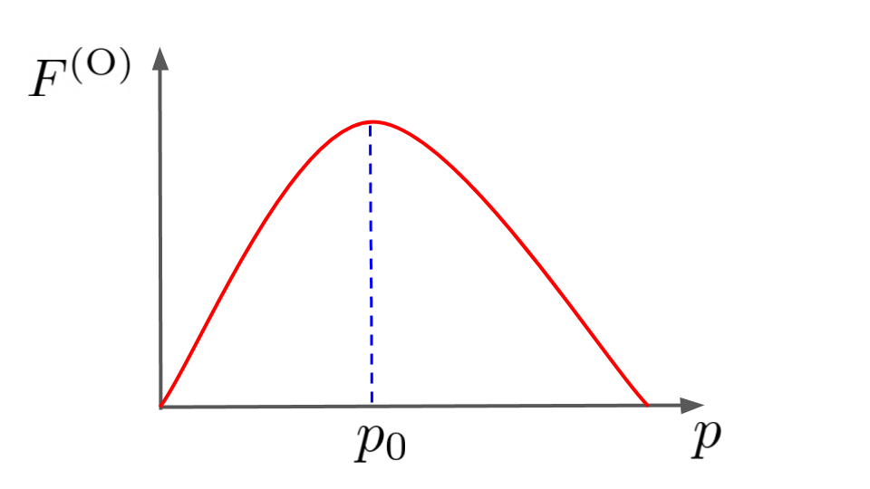
We define equivalent distribution function(EDF) as the summation of normalized distribution function weighted by their plasma frequency(squared) of the species involved.
| (37) |
where where is the plasma frequency of a reference species.
Gardner’s theorem states that a single humped equivalent distribution function(EDF) cannot support a growing set of waves.
We adopt the method of contradiction. Let us assume on the contrary that there is a wave with .
The dispersion relation in terms of the EDF can be written as
| (38) |
Subsituting we get
| (39) |
Separating the real and the imaginary part we get
| (40) |
From Fig. 11 of the EDF we have the maximum of the equivalent distribution function at which corresponds to which gives us
| (41) |
so that
| (42) |
Since and we have
| (43) |
Using B in the equation above we get ,
| (44) |
The integrand is non-negative for all values of as seen from 42. Hence, the left hand side is always greater than unity so that the equation cannot be satisfied. This proves that our original assumption must be incorrect.
Appendix C Useful derivations for the Langmuir mode
C.1 Energy distribution among Langmuir waves and particles in the plasma
Following “Introduction to Plasma Physics" by Nicholson (1983) we have
| (45) |
The above expression can be further simplified as
Using B the above expression can be further simplified to finally obtain
| (46) |
For our case we will evaluate the above expression at where the Langmuir mode touches the line. Please note the quantities for the Langmuir mode has been normalized at this frequency.
The energy distribution between particles and electric field for Langmuir mode for the relativistic pulsar plasma evaluated at the point where the mode touches the line is given as
| (47) |
Now, we have
| (48) |
Now, can be simplified as
| (49) |
For the ultra-relativistic case as is true for pulsar plasma which further simplifies to
| (50) |
Thus, can be simplified to
| (51) |
where where is the plasma frequency of some reference species.
Then we have
| (52) |
Making use of the ultra-relativistic approximation again we have
| (53) |
For a one-component plasma we have
Thus, in an ultra-relativistic plasma the electric field energy density of an electrostatic wave is much lower than the energy of oscillation of the particles. As the Lorentz factor of the particles becomes very high ,the electric field energy tends to be very very small.
C.2 Bandwidth of the growing waves
We have
| (54) |
Similarly we have
| (55) |
Using the ultra-relativistic approximation we can write
| (56) |
where
Comparing both the expressions we get
| (57) |
Again we have, from the normalised dispersion function
| (58) |
The bandwidth of the growing waves can be obtained using the constraint
| (59) |
We have
| (60) |
Thus we have
| (61) |
where
Appendix D Algorithm for numerically solving for the hydrodynamical equations and using python packages
Location of the hydrodynamic pole and the EDF: The imaginary part of the hydrodynamic dispersion relation is a corollary of the Gardner’s theorem discussed in section B. The condition can be satisfied only if of the hydrodynamic pole lies in the dip of the EDF. As discussed in A.2 the hydrodynamic pole is necessarily complex with > 0. As the dip in the EDF decreases and the growth rate also decreases until it vanishes altogether for a single humped EDF. Following this generic ideas we have carried out the following steps to solve the hydrodynamic equations.
- Step 1:
At a given we first check whether EDF is single-humped or not as shown in plot B of Fig.2,4 and 5 for ; and plots (C) and (D) for of Fig. 8 of the main paper. If it is not, the three-momenta values between the two peaks of the EDF/ dip of the EDF is divided uniformly into (n = 100) grid points to be used as guess values for . Using these we estimate guess values for .
- Step 2:
We first need the the solution () for K = 1. The guess values for is taken as K. The guess values for is taken from to uniformly divided into m = 1000 points. This gives a 2D grid with n m points such that each grid represents a guess value () for the hydrodynamic dispersion relations for K = 1. Both and are estimated for each grid point. The grid points for which were filtered to be used as guess values for the python package fsolve.
- Step 3:
The python package fsolve takes the filtered guess values () with arguments KEDF and a tolerance value . It then solves for the real and imaginary part of the hydrodynamic dispersion relation and simultaneously. It converges to a (. The solution so obtained is then inserted into the expression for and to get the residuals. We take a conservative approach wherein the solution is taken as valid only if the residuals are atleast 3 orders of magnitude lower than .
After getting a solution we can estimate by following these steps . The so obtained for K = 1 is shown as a black dashed line in plot(B) of Fig. 2, 4 and 5 ; and plot (C) and (D) of Fig.8 of the main paper.
- Step 4
After getting the solution for K = 1, the wavenumber is changed in steps of and the previous step is repeated with the difference that from now on only one guess value needs to be provided. The guess values () for the th iteration is the solution for th iteration. After a solution converges for wavenumber K = 1 + , the residuals for and are estimated. The process is terminated at a wavenumber where either or the residuals do not satisfy the criteria mentioned above, whichever occurs first.
At the end of this stage we have obtained the dimensionless dispersion relation. The first, second and third subplot of (C) in Fig. 2, 4 and 5 shows , and the residuals (numerical errors) of and as a function of K.
- Step 5
: To get the dispersion relation in the dimensionless form we estimate the scaling factor [in rad/s] via Eq. 3 of the main paper. The dispersion relation in the dimensional form is obtained by the following steps: [in rad/s] , [in s-1] and k = K [in cm-1]. The first and second subplot of (D) in Fig. 2, 4 and 5 of the main paper shows the dimensional dispersion relation ( also referred to as spectrum of the growing set of waves). The third subplot of (D) in the Fig. 2, 4 and 5 shows the group velocity dispersion [in cm2 s-1] as a function of the wavenumber k. In all three figures group velocity dispersion is positive for the growing set of waves.
- Step 6
: At a given the normalized bandwidth of the growing waves is given by . Using , , and in Eq. 9 and Eq. 10 of the main paper we obtain the maximum gain that can be associated with Re. The Re(), Re() and the gain curve are shown as upper, middle and lower subplots of panel (F) in Fig. 2, 4 and 5.
References
Nicholson D. R, 1983
Sturrock P.A , 1994