Entangled Photon-Pair Sources based on three-wave mixing in bulk crystalsPreprint: AIP/123-QED
Abstract
Entangled photon-pairs are a critical resource in quantum communication protocols ranging from quantum key distribution to teleportation. The current workhorse technique for producing photon-pairs is via spontaneous parametric down conversion (SPDC) in bulk nonlinear crystals. The increased prominence of quantum networks has led to growing interest in deployable high performance entangled photon-pair sources. This manuscript provides a review of the state-of-the-art for bulk-optics-based SPDC sources with continuous wave pump, and discusses some of the main considerations when building for deployment.
I Introduction
The nonlocal correlations of entangled systems play a central role in quantum technologies across domains as varied as communication, sensing and computation. Generating entangled states in a reliable and reproducible manner while pushing the limits of repetition rates and quality of entanglement can thus be considered a key prerequisite towards practical applications.
From an applications perspective, even the most basic form of entanglement - bi-partite entanglement in two-level quantum systems - promises to play a major role in quantum information science and technology. In the context of quantum communications for example (but also for some scenarios in sensing and information processing), entangled photon-pairs which can readily be distributed to remote parties are a basic building block for many envisioned applications.
The last two decades have seen significant efforts dedicated to the proof-of-concept demonstration and then refinement of methods for photon-pair generation on a variety of technological platforms. Technologies ranging from atom- and ion-based systems to engineered defects in solid-state devices and 2-D materials are steadily improving in performance such that the ultimate goal of scalable and on-demand emission of single- and multi-photon states is well within reach. At present, however, the most widely employed approach remain probabilistic photon-pair sources based on spontaneous wave-mixing processes in nonlinear optical materials. Decades of research in nonlinear optics have provided a vast set of tools for engineering wave-mixing processes, resulting in highly efficient and versatile photon-pair generation schemes for entanglement in a variety of photonic degrees of freedom.
The most common wave-mixing techniques employed in photon-pair sources are based on accessing either the second order () or third order () optical nonlinearities, which lead to the three-wave or four-wave mixing regimes, respectively. Higher-order wave mixing for direct generation of photon multiplets has been studied and proposed, for instance in Corona et al. 2011, yet is not commonly employed in the optical regime due to the low conversion rates but has recently been achieved in microwave systems Sandbo Chang et al. 2018. Note however, that equivalent higher-order nonlinear interactions have already been realized via cascading of nonlinearities Huebel et al. 2010.
The major differences between three- and four-wave mixing is in the magnitude of the optical nonlinearity governing the process as well as the number of fields involved in the process. The nonlinearity on which the spontaneous four-wave mixing (SFWM) process occurs is very weak and efficient SFWM sources are thus most commonly implemented in guided wave systems such as integrated photonics ring resonators, pulsed pump in single mode fibers, or highly nonlinear photonic crystal fibers Fulconis et al. 2005. Even higher nonlinear interactions may be achieved via mode-confinement in waveguides, which significantly improves the rate of photon-pair production, but also limits the degrees-of-freedom accessible. Spontaneous three-wave mixing processes (STWM), on the other hand, have much stronger optical nonlinearity and are thus routinely achieved within both bulk and waveguide optical systems.
An important feature of three-wave mixing in bulk material is the access to various degrees-of-freedom and this has been utilised to demonstrate entanglement in polarization Kwiat et al. 1995; Kwiat et al. 1999, spatial mode Krenn et al. 2017; Forbes and Nape 2019, time Brendel et al. 1999 and frequency Avenhaus et al. 2009. Moreover, these sources have been shown to provide entanglement across degrees-of-freedom simultaneously in a so-called hyper-entangled state Fujiwara et al. 2009; Ma et al. 2009. As a result of this flexibility, the spontaneous three-wave mixing process, commonly referred to as Spontaneous Parametric Down Conversion (SPDC), is a widely used tool in quantum information science implementations.
The supporting technology needed for implementing SPDC are readily obtainable and setups work reliably at room temperature. The components can be easily modified to explore multiple applications. For these reasons, bulk-based SPDC systems have a higher technological maturity when compared to waveguide based systems Meyer-Scott et al. 2018; Orieux et al. 2017; Huber et al. 2018.
In this review article, we focus mainly on the development of entangled photon sources based on the process of SPDC in bulk nonlinear materials, and make a brief comparison to waveguided SPDC. For a more detailed discussion of nonlinear quantum optics on integrated platforms, we refer the interested reader to the comprehensive review articles, see e.g. Vergyris et al. 2017. Furthermore, we will primarily discuss continuous wave pumped SPDC, where the pump is generally considered a monochromatic wave. In particular, SPDC pumped with ultra-fast laser pulses is widely used in studies of multi-partite photonic entanglement where the sub-coherence pumping Żukowski et al. 1993 allows the coherent interaction between multiple photon-pairs. This technique has been used for instance in the implementation of four-photon entanglement Pan et al. 2001, or quantum state teleportation Bouwmeester et al. 1997, and we refer the reader to the following review article Pan et al. 2012. We begin with a description on the principles governing SPDC production, followed by identifying the relevant performance parameters for an entangled photon source (section II). We provide a detailed description of polarization entangled photon sources in different phase-matching geometries in section III. In section V, we discuss the progress of entangled photon sources in other degrees of freedom. Finally, our review will conclude with a discussion of the main application areas for entangled photon sources and an outlook (section VI).
II Spontaneous Parametric Down Conversion
The response of a dielectric medium to an electromagnetic field is given in terms of polarization of the material written as a sum of electric fields
| (1) |
where is the vacuum electric permittivity, is the linear susceptibility and are the nonlinear susceptibilities of the medium. The second order () process enables three electromagnetic fields to interact in a non-centrosymmetric medium leading to a transfer of energies between the fields. This is known as three-wave mixing. The specific case where the two lower energy fields are initially vacuum modes is known as Spontaneous Parametric Down Conversion and is illustrated in Fig. 1.

The process is spontaneous as there are no input signal and idler photons to stimulate the process, but only the inherent vacuum fluctuations of the modes. SPDC is therefore a direct manifestation of the quantized description of the electro-magnetic fields. The term parametric refers to the fact that the interaction medium does not add or subtract energy or momentum in the process.
II.1 The Interaction Hamiltonian
The Hamiltonian governing SPDC inside an nonlinear interaction volume can be written as Mandel and Wolf 1995; Glauber 2007; Ou 2007; Torres et al. 2011:
| (2) |
The interaction of the pump and target fields is commonly expressed using the non-depleted pump approximation. This is appropriate as the susceptibility has a very small magnitude, and most of the pump energy is not down converted. The non-depleted pump field with wave-vector and frequency may be expressed classically as
| (3) |
where = is the normalization factor, is the spatial mode of the pump in transverse momentum coordinates , is the spectral function and is the polarization vector of the pump. This expression is generally known as the squeeze-operator Loudon 1983, and SPDC is considered as the result of the squeeze-operator acting on vacuum modes, and thus the output states of SPDC are also referred to as squeezed vacuum. The electric field operators for the signal and idler photons have the form
| (4) |
where = is the normalization factor and , are the respective refractive indices and polarization vectors. The quantum state of SPDC output at time is then given by
| (5) |
where is the initial vacuum state. The Taylor series expansion of the above equation suggests that multi-pair events in SPDC are possible Takesue and Shimizu 2010; Takeoka et al. 2015; Tsujimoto et al. 2018a, with a strong dependence on pump power. The probability of single pair emission is obtained by assuming the weak-pump regime, which allows to truncate the series expansion to first order,
| (6) |
Keep in mind that the higher-order emissions (multi-pair emissions) of SPDC must be considered in some scenarios as they could reduce the entanglement quality at sufficiently large pump intensities. The general description of the bi-photon state emitted by SPDC (or squeezed vacuum) is Loudon 1983; Braunstein and van Loocuk 2005
| (7) | |||||
where are the photon number states in the signal and idler modes, , and is the interaction parameter in the Hamiltonian. In many applications of SPDC pair sources the truncation to single-pairs is a valid approach because the interaction strength is chosen relatively low, e.g. , less than 1% of all emission events contain more than one photon-pair.
The integral in (6) can be evaluated by decomposing the respective wave-vectors into transverse and longitudinal components. The integral is explicitly written as
| (8) |
One simplifying condition is that the pump and SPDC transverse modes are much smaller than the cross-section of the non-linear material, which is usually a crystal. The crystal structure further reduces the susceptibility tensor to a single coefficient where . Over a suitable interaction time, the integral along the crystal volume can be expressed as
| (9) |
where is the SPDC mode function given by
| (10) |
The effective nonlinear coefficient is now
| (11) |
and = is the longitudinal wave-vector mismatch. The mode function in Eqn.(10) obeys energy and momentum conservation :
| (12) | ||||
| (13) | ||||
| (14) |
The transverse function of the pump and targeted SPDC modes can be modeled in order to optimize brightness and heralding efficiency in practical sources Ling et al. 2008; Bennink 2010. Note that for a continuous-wave pump (monochromatic), , which will further simplify the bi-photon mode generated by SPDC, expression (10). If the SPDC pump is a wide-band and/or pulsed laser, the bi-photon mode will have an internal structure and potentially have mixed spectra, which has been extensively studied, see for instance Grice and Walmsley 1997; Pan et al. 2012.
Based on phase-matching geometry, SPDC sources have collinear or non-collinear emission of photon-pairs. Figure 2 shows the wave-vector diagrams for collinear and non-collinear cases of phase-matching. Here, and are the angles of signal and idler wave-vector with reference to the pump, which are different for non-degenerate photon-pairs. is the mismatch among the pump, signal and idler wave-vectors, mathematically expressed as . This wave-vector mismatch has great significance in designing entangled photon sources.
II.2 Phase matching techniques
When using bulk crystal SPDC there are two main ways to achieve phase-matching: (a) by exploiting birefringence to compensate for phase mismatch, or (b) using periodic poling of the material which leads to quasi-phase matching (QPM). Typically this involves at least one of the fields propagating at an angle with respect to the optical axis (critical phase matching configuration), and the resulting transverse walk-off limiting the maximum interaction length for the process. The more desirable non-critical phase matching condition, where propagation of all fields is along an axis perpendicular to the optical axis is usually only fulfilled for very specific materials and wavelength combinations. Alternatively, non-critical collinear interaction can also be achieved quasi phase-matching in periodically-poled nonlinear materials. All of these methods try to achieve the momentum conservation condition:
| (15) |
This condition cannot be achieved with normal dispersion but requires the above mentioned approaches, i.e. either materials exhibiting birefringence, or the use of quasi-phase matching. Note that SPDC in waveguides can also make use of the propagation parameters of guided modes to achieve modal phase-matching, as will be discussed later.
In a birefringent optical material, the wave polarized orthogonal to the principal plane is denoted as ordinary () beam and the wave polarized along the plane is denoted as extra-ordinary (). For commonly used uniaxial crystals the refractive index of the ordinary wave () is independent of the orientation of its wave-vector inside the crystal, whereas the extra-ordinary refractive index depends on the angle between the wave-vector and the optic axis (). In sources based on biaxial crystals the orientation of all wave-vectors to the optic axis must be considered Boeuf et al. 2000. This effective extra-ordinary refractive index is expressed as:
| (16) |
Critical phase matching is then achieved by tuning the angle of the pump wave vector with respect to the optic axis. There are two possible configurations known as type-I or type-II. In type-I phase-matching the generated photon-pairs are co-polarized with their polarization orthogonal to that of the pump. In type-II, the photon-pairs are orthogonally polarized to each other.
The other phase-matching technique is quasi phase-matching (QPM) where there is a spatial modulation of the linear and nonlinear properties in the medium along the propagation direction Fejer et al. 1992. A common QPM method uses periodic flipping of the crystal lattice orientation to achieve an effective nonlinearity. This method makes use of a multi-domain material, unlike in critical phase-matching where the entire material is a single domain with the optical axis fixed in one direction. Moreover, the periodic domains compensate the spatial walk off between the three waves which effectively increases the interaction length Shichijyo et al. 2004.

Due to this periodic domain structure the intensity of generated photons grows in a step-wise manner along the interaction medium (Fig. 3). The phase mismatch in QPM is mathematically expressed as
| (17) |
Here, , is the phase mismatch of the bulk material. The grating wave-vector has a magnitude of , with being the grating or poling period. This grating wave-vector allow us to engineer the spectral and spatial properties of the down-converted photon-pairs. Moreover, QPM can allow type-0 phase matching where pump, signal and idler photons are co-polarized.
II.3 Basic performance parameters for photon-pair sources
This section discusses the performance parameters commonly used to characterise photon-pair sources.
1. Brightness: The brightness of a source is defined as the number of pairs produced in one second for unit pump power typically written as the number of pairs/s/mW. The intrinsic brightness of a source can be traced back to the nonlinear coefficient of the material which determines the probability that a pump photon will be converted to a photon-pair Ling et al. 2008. It is important to make a distinction between observed and generated brightness. The observed brightness is highly dependent on heralding efficiency (see below) and other system parameters such as detector efficiency. The generated brightness can often be inferred once the system losses are taken into account. In terms of applications, the observed brightness is often the more relevant parameter.
The SPDC process is typically a broadband process, and for specific application it is important to understand the spectral brightness where the typical unit is pairs/s/nm/mW. This is the brightness divided by the spectral bandwidth of the SPDC output. It should be noted that brightness values reported for SPDC sources often ignores the contribution of multiple pairs, and so is valid only in the weakly pumped regime.
2. Heralding efficiency: Here, we define the heralding efficiency as the ratio of observed coincidence counts to the signal/idler counts 11 1 In the context of heralded single photon generation, the heralding efficiency is typically normalized with respect to detection efficiency.. This parameter, also known as the coincidence-to-singles ratio or Klyshko efficiency, is a very practical and readily accessible performance estimator that depends upon both the efficiency of collection and detection. Note that, while detectors can be changed in principle, the collection efficiency is closely related to the spatial properties of the SPDC emission, specifically the spatial mode distribution of the signal (idler) conditioned on the partner photon coupling into a specific spatial mode Bennink 2010, 22 2 In the context of characterizing the spatial mode distribution in the SPDC process, the concept of conditional spatial mode overlap, may also be considered equivalent to the heralding efficiency.. The number of photons registered by signal () and idler () detectors for a given resolution time are given by Takesue and Shimizu 2010
| (18) | ||||
| (19) |
and the rate of coincidence events between the two detectors is
| (20) |
where is the number of photon-pairs produced in the given resolution time and , are the heralding efficiencies of signal and idler respectively. The heralding efficiencies are expressed as and , where and are the detection and collection efficiencies.
II.4 Photonic Entanglement and its experimental measures
In this article, we mainly focus on two qubit entanglement in different degrees of freedom such as polarization, time bin etc. The target state of such entangled photon-pair sources fall to any of the maximally entangled bell states, given as
| (21) |
The and are two orthogonal states. Below we discuss some of the experimentally observable measures of entanglement.
Polarization correlation visibility / contrast:
Entangled photon-pairs exhibits non-local correlation which can be observed from their measurement outcomes. In case of polarization entanglement, signal and idler photons are projected to different linear polarization states
| (22) |
The probability of finding the entangled photon-pair in the projected state is given by
| (23) |

To examine polarization entanglement, polarization in one arm is projected to one among the four horizontal, vertical, diagonal or anti-dagonal polarizations represented by the states , , or respectively, and the coincidence counts are plotted for different polarizer angles of the second arm. Figure 4(a) represents the polarization curves corresponding to the Bell state . The polarization visibility for each basis is determined by the expression
| (24) |
where and are the maximum and minimum values of the curve in a given measurement basis. A major contribution to error when estimating visibility is the rate of accidental coincidences across the detectors, due to stray light, multi-pair emissions and internal detector noise. The rate of accidental coincidences is approximated as
| (25) |
where is the coincidence window used in coincidence counting. By subtracting , the rate of true coincidences can be determined. Note that the Eqn. (25) is an approximation which works for lower values of heralding efficiencies. In the regime of high photon pair rate and higher detection efficiencies, accidental coincidences due to multi-pair emission needs to be accounted separately for estimating the visibility Takesue and Shimizu 2010. Many single photon detectors exhibit saturation behaviour at higher detection counts and this needs to be addressed while estimating the accidental coincidences Grieve et al. 2016.
Note that it is also possible to obtain practical estimates on the quality of entanglement using only common polarization measurement acting on both signal and idler photons. This is particularly useful for quick characterization of entangled photon-pair sources in collinear design using a single polarizing element that is placed in the common path of the co-propagating signal and idler photons. For example, in Villar et al. 2018, it is shown that a joint linear polarization measurements allow to differentiate the state from or a mixed state by observing the polarization correlations. The photons prepared in state are co-polarized in one basis (H/V) and anti-polarized in the other linear basis (D/A). So, in the case of , the curve from single polarizer measurements show high contrast between minima and maxima, while show a constant pair rate for any polarizer setting (Fig. 4(b)). Similarly, for maximally entangled states of the form , recording the visibility of coincidence fringes over the relative phase (e.g. by tilting a birefringent plate or a Soleil Babinet compensator) it is possible to certify entanglement with a common diagonally oriented polarizer in the signal and idler path Steinlechner et al. 2017.
Bell’s inequality:
The violation of Bell’s inequality is one of the most commonly used parameters to qualify or witness polarization entanglement. An experimentally very accessible form of Bell’s inequality is given by the inequality proposed by Clauser, Horne, Shimony, and Holt (CHSH) in 1969 Clauser et al. 1969. The CHSH version of Bell’s inequality is expressed as
| (26) |
where correlation values, , can conveniently be normalized using the measured coincidences given by Aspect et al. 1982
| (27) |
Here is the coincidence counts for each polarization angle and . All Bell states clearly violates the inequality given in Eqn.(26). For example, consider a source emitting polarization entangled photons in the state . Substituting the probability corresponding to the state from Eqn.(23) in Eqn.(27), we obtain for angles = , = and = . The CHSH values can be estimated from the visibility curves (Fig. 4).
State fidelity:
The quantum state fidelity determines the closeness of the experimental quantum state expressed by the density matrix to a particular target state expressed by the density matrix . It is mathematically expressed as
| (28) |
will have values ranging from 0 to 1 depending on the overlap of the experimental with the desired target state. For an ideal state , . Typically, the experimenter’s goal is that the target state be a pure maximally-entangled Bell state. In this case, one often refers to the Bell-state Fidelity or simply the entanglement fidelity of a state. The Bell-state fidelity of a classical mixed state to the maximally entangled state is 0.5. In order to determine how to calculate the Bell state Fidelity, let us first consider the density matrix of a perfect target state for example, the density matrix of the Bell state :
| (29) |
In order to evaluate the Bell state Fidelity of the two-photon SPDC state produced in the source according to the definition above, we must first reconstruct the experimental density matrix . This can be accomplished by performing a series of polarization correlation measurements on the two photon state. In general, at least 16 such polarization measurements are required to reconstruct the density matrix using a procedure called quantum state tomography. However, errors and noise in the measurement data can lead to unphysical density matrices. A physically allowed density matrix can be obtained using maximum likelihood estimation Banaszek et al. 1999; James et al. 2001. For more detailed description of the experimental estimation of photonic qubits, the reader may refer to Ref. Altepeter et al. 2005a.
The aforementioned procedure is not always the most efficient way of characterizing entanglement generated in an SPDC source. Whenever the fidelity of an unknown experimental state with a particular Bell state is the main property of interest, then a complete reconstruction of the density matrix is not strictly required. From the properties of the density matrix, it can be shown that the following expression Jennewein et al. 2009; Gühne and Tóth 2009 gives the the Bell-state fidelity as:
| (30) |

where refers to the absolute values of the two-photon correlation functions in three mutually unbiased measurement bases (here linear H/V, D/A and circular L/R), each of which can derived from four protective measurements, thus requiring only a total of 12 settings. Note that when a lower bound on the Bell-state fidelity is sufficient the number of required measurements can be further reduced. It can be shown Steinlechner et al. 2017 that the Bell-state fidelity is lower bounded by experimental visibilities in two mutually unbiased measurement bases, e.g. in the linear horizontal vertical and diagonal/antidiagonal bases via the relation:
| (31) |
Other frequently employed measures of entanglement are the tangle and the concurrence, and entanglement of formation Coffman et al. 2000; Wootters 1998. The concurrence can be calculated from the tomographically reconstructed density matrix, or lower bounded via:
| (32) |
The entanglement of formation is particularly relevant to quantum information processing as it has clear operational meaning; the entanglement of formation represents the minimal number of maximally entangled bits required to produce produce the state via local operations and classical communication (LOCC) procedure. The entanglement of formation may be lower bounded by the concurrence according to:
| (33) |
The interested reader is referred to Refs. Gühne and Tóth 2009; Horodecki et al. 2009; Bavaresco et al. 2018 for more detailed discussion on measures of entanglement, in particular extension to high-dimensional and multi-partite entanglement.
III Polarization Entangled photon-pair sources - variations on a theme
Photons generated via SPDC in a single decay channel are not inherently entangled in the polarization degree of freedom. To see how we may obtain polarization entangled photon-pairs, let us consider two generic SPDC sources, each producing orthogonally polarized photon-pairs in a sate and , where the labels (1,2) denote any spatial, spectral, or temporal features of the respective source. In many experimental settings these properties are not directly accessible, e.g. the characteristic features of the temporal wave function occur on the ps timescale, whereas the detectors’ timing resolution is on the order of ns. In order to determine the experimentally accessible polarization correlations for the combined SPDC emission from the two sources
| (34) |
let us consider the result of a joint projective polarization measurement of the signal and idler photons in a local superposition basis . The probability for coincidence detection is given by
| (35) |
Hence, if the photon-pairs emitted from the two sources are distinguishable, i.e. the labels correspond to orthogonal states (), the phase- dependent term vanishes, and we can not observe the characteristic non-local coherence of a polarization-entangled state. In order to directly obtain a maximally entangled Bell state , the labels indicating the source of origin must factor out of the picture. Only then can we consider the state as coherent superposition of two, otherwise identical, orthogonal polarization states and .
Engineering the pairs to exhibit polarization entanglement is thus generally associated with the concept of a ’quantum eraser’ Scully and Drühl 1982; Scully et al. 1991; Aharonov and Zubairy 2005 to remove any distinguishing features. These concepts have been applied to polarization entangled photon sources by using one or two beam splitters (Fig. 5(a)) to erase the photon path information. The photons are detected after the beam splitter(s) and the non-local correlations can be observed by employing post-selection and only considering a certain subset of all possible detection outcomes. This approach, while elegant, however reduces the efficiency of the source by at least 50% and is therefor not suitable for loophole-free Bell-tests. First demonstrations of entanglement from single-path SPDC include the work by Ou and Mandel 1988 Ou and Mandel 1988a or Rarity and Tapster in 1990 Rarity and Tapster 1990.
By using nonlinear interferometers Chekhova and Ou 2016, researchers have come up with a large variety of entangled photon-pair sources. What follows are the general steps to be taken when realizing a polarization entangled photon-pair source.
Selection of two pump decay paths:
Two decay paths with orthogonal polarization states from Type-I/0 ( and ) or Type-II ( and ) phase matching are used. In any case, the two decay paths must be indistinguishable in spectral and spatial modes. It is important to note that the pump decay paths can occur within a single process (e.g. from a single crystal Kwiat et al. 1995), or from different processes (in different crystals e.g. crossed crystal source Kwiat et al. 1999).
Superposition:
The two decay paths need to be put in a coherent superposition to obtain the entangled state. This can be achieved by using regular or polarizing beam splitters. In Fig. 5(a), the interference of orthogonally polarized photons from two input ports of the beam splitter generates entanglement after post-selection. Two orthogonally polarized photon-pairs each at the two input ports of a polarizing beam splitter can be superposed to generate entangled state, as shown in Fig. 5(b). Superposition can also be achieved by making use of spatially overlap from beam walk-off within birefringent crystals (Fig. 5(c)). Spatial filtering (using pinholes or single mode fibers) can be used to remove residual spatial distinguishability.
Temporal compensation:
SPDC is a broadband process which allows phase-matching over a broad spectrum of wavelengths. In many source configurations, the generated SPDC output travel through dispersive materials where the photon-pairs will pick up a wavelength dependent phase. This results in spectral distinguishability, and thereby reducing the quality of entanglement. This wavelength dependent phase can be removed by employing additional ’compensation’ crystals (e.g. Yttrium orthovanadate, YVO4,). Methods of temporal compensation using birefringent crystals is illustrated in Fig. 5(d).
Splitting:
The signal and idler photons must be separated before they are useful for downstream applications. These photons can be separated by emission angle Kwiat et al. 1995; Kwiat et al. 1999, polarization property Kim et al. 2006, or wavelength Hentschel et al. 2009. Emission angle splitting is typically associated with non-collinear SPDC. However, this is also possible in collinear cases where the signal and idler can be split using a wedge mirror Perumangatt et al. 2020; Lohrmann et al. 2020, as shown in Fig. 5(e). Many modern sources prepare the signal and idler photons with different wavelengths (non-degenerate) for easy separation. For wavelength based separation, dichroic mirrors are a natural choice (Fig. 5(f)). However, many dichroic mirrors comes with group delay dispersion which introduce additional wavelength dependent phase between and polarization states degrading the quality of entanglement. Wavelength division multiplexers (WDM) based on fused fibers employing evanescent coupling are an alternative technology for splitting the two wavelengths without introducing the wavelength dependent phase Trojek and Weinfurter 2008; Steinlechner et al. 2013 (Fig. 5(g)).
In the following we detail concrete examples involving these basic steps in a variety of geometric arrangements and phase-matching configurations.
Non-collinear phase-matched sources
Photon-pair sources with non-collinear emission can be grouped into three general types: 1. Single pass of the pump through a single crystal, 2. Single pass of the pump through two crystals, and 3. Two pump passes through a single crystal. In these sources, the signal and idler photons have degenerate wavelengths. The major characteristics for each category are discussed below.
III.0.1 Single crystal, single pass configuration
In this geometry,
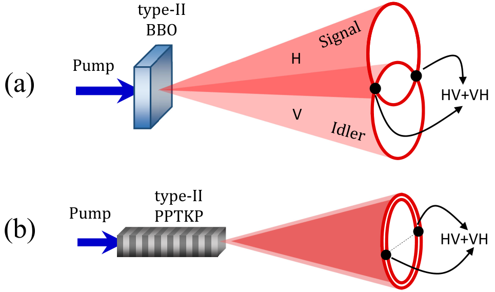

type-II phase matching is preferred where a single crystal emitting photon-pairs polarized orthogonal to each other can be a source of polarization entanglement (Fig. 6) Kwiat et al. 1995; Trojek et al. 2004. The signal and idler photons are emitted in separate cones, which can be made to intersect at two points where the polarization of the emitted photon is undefined (Fig. 6(a)). The photon-pairs collected from these intersection points are entangled in polarization with the state
| (36) |
By using a type-II quasi phase-matched crystal, the same state can be obtained, but where the signal and idler cones complete overlap (Fig.6(b)). This geometry has been very popular with a large number of ground-breaking experiments adopting the design. Its simple alignment requirements, and small part number also make it a useful teaching tool. The quasi phase-matching allows access to higher nonlinearity leading to a relatively brighter source Fiorentino et al. 2005; Lee et al. 2016. Overlap of two concurrent type-I QPM structures in a single crystal can produce highly non-degenerate entangled photon-pairs de Chatellus et al. 2006.
The temporal walkoff between ordinary and extra-ordinary photons travelling through the crystal degrades the entanglement. This is corrected by the use of a half-wave plate and a compensation crystal that is half the thickness of the SPDC crystal Kwiat et al. 1995 (Fig. 7(a)-(c)). This compensation technique partially corrects for spatial walk-off (Fig. 7(d)). The source can act as a ’universal Bell state synthesizer’ if a half-wave plate is introduced in one arm and the two paths are combined at a polarizing beam splitter Kim et al. 2003.
Focusing of the pump brings the SPDC conditions towards the thick-crystal regime, and the spatial-walkoff can be quite pronounced Lee et al. 2005. However, with proper spatial filtering, the entanglement visibility can be preserved at the cost of the brightness. In general, type-II non-collinear SPDC sources employ Barium Borate (BBO) as the nonlinear material. The brightness of the sources could be improved by using other materials with a larger nonlinear coefficient, e.g. Bismuth Borate (BIBO) Halevy et al. 2011.
III.0.2 Double crystal, single pass configuration
Polarization entanglement can be achieved by superposition of photons from two successive non-linear crystals. This geometry accepts both type-I and type-II phase matching. This technique was first reported using two thin Type-I BBO crystals Kwiat et al. 1999 (Fig. 8(a)). A diagonally polarized pump photon incident on the crossed crystals have an equal chance to be down converted in either crystal. These two possible SPDC processes are coherent, and when their spatial output overlap, the photon-pairs can be in the maximally entangled state
| (37) |
This geometry enables non-maximally entangled states White et al. 1999 by tuning the pump polarization. Various optimization techniques can be found in the literature Migdall 1997; Rangarajan et al. 2011a; Nambu et al. 2002; Rangarajan et al. 2009; Rangarajan et al. 2011b.

Apart from the original scheme using two crossed crystals, there has been several other two crystal alignment techniques that have been studied. In Ref.Bitton et al. 2002, two crystals are used with flipped optical axes (Fig. 8(b)). The emission cones with orthogonal polarization overlap completely removing the dependence of photons’ polarization on their azimuthal positions within the cone. This ensures entanglement of photon-pairs at any point of the cone if proper temporal compensation is used. Since polarization of the pump is same for both crystals, this doubles the brightness of the SPDC output compared to Kwiat et al. 1999. Instead of emission cones, overlapping of beam-like emission from two crystals can also be used Niu et al. 2008 (Fig. 8(c)). Finally, a thin half wave plate sandwiched between two type-II parallel crystals can also give a beam-like emission of entangled photon-pairs Zhang et al. 2015a (Fig. 8(d)). Notice that in all of these configurations, the pump field driving the second pair-emission process, co-propagates with the SPDC emission from the first source. In configurations with a common optical path for pump, singal and idler, phase shifts due to changes of the path length between the two SPDC emitters perfectly cancel, and do not contribute to the overall phase of the polarization-entangled state. This auto-compensating feature of ’common-path configurations’ leads to long-term stability without the need for active interferometric stabilization.
III.0.3 Single crystal, double pass configuration
Another method for entanglement generation is to use two paths for the pump beam within the same crystal. There have been two schemes using this method. In the first scheme Herzog et al. 1994; Herzog et al. 1995; Vallone et al. 2009, the pump, after passing through a type-I crystal, is reflected back (Fig. 9(a)). Additional mirrors reflect the photon-pairs from the first pass to overlap with the output of the second pass producing the state , where is the phase difference from the path length differences. Since any changes in the path length of the pump and the SPDC photons will also contribute to changes in this phase shift, interferometric stability of the system is required. This poses a critical challenge, which is not present in two-crystal configuration.

It has been shown that this scheme can be utilized for optimal generation of pulsed entangled photon-pairs that give better quantum interference visibility even without spectral filtering Hodelin et al. 2006.
The second scheme (Fig. 9(b)) employs a quasi phase-matched crystal inside a polarizing Sagnac interferometer Slussarenko et al. 2010. This can be realised using a Type-0 PPKTP crystal with either continuous-wave Jabir and Samanta 2017 or pulsed Kim et al. 2019 pump. Counter-propagating pump beams in the interferometer generate photon-pairs in the state . In one arm, an achromatic half-wave plate (denoted as aHWP) rotates the polarization of all beams. The photon-pair passing through the aHWP will flip its polarization to the state. The output from both arms combine at the PBS to give the state . The notations & are used to distinguish the propagation direction with the loop. The inherent symmetry of the Sagnac loop configuration thus removes the need for additional compensation optics. Fine-tuning of the SPDC overlap can be done by adjusting the crystal position inside the loop.
Collinear phase-matched sources
Non-collinear emission of entangled photon-pairs enable straightforward separation of the photons, but are generally more complicated to align and also need a larger footprint. Collinear emission simplifies the collection leading to brighter and potentially more compact sources. Collinear photon-pair sources found in the literature can be grouped into the same categories as the non-collinear sources apart from a recent design using a double pump pass through two crystals.
III.0.4 Single crystal, single pass configuration
One of the earliest sources in this configuration made use of type-II SPDC with a temporal walk-off compensation crystal Kuklewicz et al. 2004; Zhou et al. 2013.

In the original implementation, the entangled state was post-selected from the output of a 50:50 beamsplitter (Fig. 10(a)). We note that post-selection can be avoided if nearly collinear signal and idler photons could also be separated using their momentum correlations Prabhakar et al. 2020 (see Fig. 5(e)).
A different approach uses two different poling periods in the same crystal. There are two reported schemes. In the first scheme, two halves of the crystal have different poling periods (Fig. 10(b)), while the second scheme employs a phase-modulated structure with two interlaced poling periods (Fig. 10(c)). In both cases, the non-degenerate photon-pairs emitted due to first poling period () are orthogonal to the pairs from second poling period (). The collinear propagation of both pairs gives the state
| (38) |
A third approach is to convert the intrinsic position correlations in SPDC into polarization entanglement Shimizu et al. 2008; Perumangatt et al. 2020. For example, in a single type-0 PPKTP crystal (Fig. 11), photon-pairs may be generated in either the upper or lower half of the interaction volume. Using a segmented half-wave plate to swap the polarization state of photon-pairs from one half, followed by an -BBO crystal to overlap the output will generate an entangled state.

This can be very compact as this geometry requires minimal components, and in principle can be extended to other physical systems (such as four-wave mixing in atomic vapor) with an extended interaction volume.
III.0.5 Double crystal, single pass configuration
An early approach used a polarizing Mach-Zehnder interferometer (MZI) with a SPDC crystal in each arm (Fig. 12(a)). Kim et al. 2001; Kwiat et al. 1994; Shapiro and Wong 2000. Entangled photons in all four Bell states can be generated with this scheme by selecting appropriate phase-matching combined with the correct type of (non-)polarizing beam splitter (Fig 12(b) & (c)).

Instead of building an interferometer, a single diagonally polarized pump can act on two crossed crystals to produce collinear photon-pairs in the state . An early attempt for this configuration used two vertically stacked crystals with a diagonally polarized pump passing through both of them equally to generate entangled photon-pairs (Fig. 12(d)) Shi and Tomita 2003. A similar method uses horizontally stacked crossed-crystals instead of vertical stacking to produce collinear photon-pairs (Fig. 13(a)). This approach can use thick crystals to give high collection efficiency and brightness as the spatial walk-off can be readily compensated Septriani et al. 2016. The wavelength dependent phase associated with the pump and the SPDC photons are independently compensated using two YVO4 crystals each in the pump and SPDC paths. This scheme enables the use of a broadband pump.
When performing critical phase-matching there are always spatial walk-off effects. This is more pronounced when two crossed crystals are used because the walk-offs are not in the same direction and produce an elongated SPDC output (Fig. 13(d)).

To get the centres of the output to overlap, additional crystals must be used. Complete spatial mode overlap of the SPDC output is obtained in the “parallel-crystal” geometry (Fig. 13(b) & (e)). In contrast to the crossed-crystal scheme where only half of the pump power is used in each crystal, the parallel-crystal configuration utilizes the full pump power. One drawback of using parallel crystals is that a broadband pump cannot be used. The elongated SPDC output can be avoided using quasi phase-matching Pelton et al. 2004; Ljunggren et al. 2006; Hübel et al. 2007; Steinlechner et al. 2012; Scheidl et al. 2014 (Fig. 13(c) & (f)).
Using periodically poled crystals also enables type-0 and type-II phase-matching. In all cases, however, the wavelength of the SPDC output from both crystals must be matched carefully. For critical phase matching, the angle tuning and stability is important, while for periodically poled materials, it is the temperature control that must be maintained.
III.0.6 Single crystal, double pass configuration
In the collinear emission type sources, another way to obtain two different decay paths is to propagate the pump beam twice through the same SPDC material. This avoids having to compensate for material defects in different crystals (assuming the single crystal is uniform). This section reviews the set of schemes that use a double pass through the same crystal and they all employ interferometric techniques such as the Michelson, Mach-Zehnder and Sagnac designs. In some of these cases, the full pump power can be used in each pass, leading to brighter sources.

Figure 14(a) shows the folded Mach-Zehnder scheme where entangled photons are generated by bidirectional pumping of a single crystal Fiorentino et al. 2004. The photons generated in each direction are filtered out using dichroic mirrors. An additional arm manipulates the photon polarization before recombination to produce the entangled state . This scheme can also work with type-0/I crystals König et al. 2005.
The major disadvantage of the scheme in Fig. 14(a) is that it requires two different interferometers to be stabilised. Common-path interferometers based on the Sagnac design Anderson et al. 1994) have improved stability. The first entangled photon source using this scheme employed a type-I BBO crystal with post-selection at a beam-splitter Shi and Tomita 2004. Modern designs, however, do not need post-selection and instead use a polarization beam splitter as the first element (Fig. 14(b)). This polarizing Sagnac configuration Slussarenko et al. 2010 is currently one of the most common sources in modern studies as it supports the use of all types (0,I & II) of phase-matching Kim et al. 2006; Fedrizzi et al. 2007; Kuzucu and Wong 2008; Predojević et al. 2012; Hentschel et al. 2009; Steinlechner et al. 2014. This design also has progressed to field deployment Beckert et al. 2019, and has been demonstrated on the Micius spacecraft Yin et al. 2017a.

The Sagnac scheme has advantages in stability, but has a larger physical footprint as there is always an enclosure that is unused. Furthermore, the separation of the pump beam into two parts means that the SPDC production in each arm is not utilising the full pump power. A compact and bright source fully utilising the pump power is the “folded-sandwich” design (Fig. 15) Steinlechner et al. 2013; Steinlechner 2015. The folded-sandwich design uses less components and the full pump power is utilised in each pass. To date, this design holds the record in the literature for detected brightness. The design is not intrinsically stable and generally requires active stabilisation.
To combine the advantages from the previous designs, i.e. better stability and reduced physical footprint, it is possible to use the concept of a linear displacement interferometer (Fig. 16). In this scheme, the pump does not backtrack on itself, but takes two distinct paths through the material.

One approach uses a loop-back configuration (Fig. 16(a)) where the pump beams pass through two different regions of the same crystal. The design uses achromatic waveplates to manipulate the polarization of both pump and SPDC photons. This particular Sagnac design can be used for all phase-matching types. The other approach would separate the pump beams laterally to propagate in the same direction through a type-0 PPKTP crystal Fiorentino and Beausoleil 2008; Lohrmann et al. 2020 (Fig. 16(b)). This linear beam-displacement interferometer is intrinsically very stable. In a similar configuration, the two laterally displaced pump beams can also be passed through a type-II PPKTP crystal to produce entangled photons after combining signal photons and idler photons separately using two beam displacers Evans et al. 2010.
III.0.7 Double crystal, double pass configuration
When two crossed crystals are oriented in a polarizing Sagnac loop, entangled photon-pairs can be obtained using time-reversed Hong-Ou-Mandel interference Chen et al. 2007 (Fig. 17).

This enables photon-pairs with the same color to be deterministically separated without using dichroic mirrors or momentum correlations. This was first reported for fiber-based systems, but has also been implemented for bulk crystals Chen et al. 2018a.
A modified linear interferometric source based on double displacement technique was recently introduced Horn and Jennewein 2019 (Fig. 17). In this scheme, two beam displacing (BD) crystals are used in the input and output and this can also achieve spatial and temporal balance, leading to a high quality entangled photon-pair output.
III.0.8 Polarization-entangled photon sources based on cavity-enhanced PDC
Typically, single-pass SPDC produces photon-pairs with a bandwidth that corresponds to the phase mismatch which typically spans several GHZ. The bandwidth of these sources can be reduced by passive filtering using narrow-band spectral filters or by placing the SPDC-crystal inside a resonator. The advantage of the passive filtering approach is its flexibility - almost any spectral profile can be ’cut out’ from the emission spectrum. However, in order to counteract the filter losses that occur in this process, a correspondingly high number of emitted photons is required.
Alternatively, it is also possible to imprint the desired spectral characteristics on the generation process itself, by embedding the nonlinear medium in a resonant cavity. In this case, the cavity finesse and the ratio of its free-spectral range with respect to the natural phase-matching bandwidth - as well as which of the fields are on resonance - all act together in determining the photons’ spectral properties. Depending on how many of the interacting fields are resonantly enhanced, one distinguishes between singly-, doubly-, and triply resonant cavity PDC configurations.
When the signal and/or idler photons are on resonance, the SPDC emission is squeezed into frequency modes permitted by the optical cavity, resulting in a series of emission peaks with reduced spectral bandwidth. Cavity enhanced SPDC thus prolongs the coherence time of the created photon-pairs Ou and Lu 1999 and enhances the spectral brightness within the resonance bandwidth by a factor of up to , where is the Finesse of the resonator. Another advantage of this approach is that locking the cavity to another material system, allows to produce entangled photons that spectrally match another quantum system of interest such as atoms or ions which are relatively narrow band of just a few MHz.
Since the first theory papers on this topic, several groups have reported on narrowband photon-pair sources based on cavity-enhanced SPDC. A detailed account of the body of experimental research is beyond the scope of this article, andcan be found in Ref. Slattery et al. 2019. Section IV merely highlights some of the work on polarization-entangled photon sources with cavity-enhancement.
In 2000, Oberparleiter et al. demonstrated a SPDC source for polarization entangled photons with a pump cavity Oberparleiter and Weinfurter 2000, thereby enhancing the effective pump power for a 2 mm BBO crystal by a factor of 7, while observing a polarization correlation visibility of up to 96%. The bandwidth of the 702 nm SPDC photons remained relatively broadband, about 5 nm FWHM.
Producing narrow-band SPDC, on the other hand, requires a cavity for the SPDC signals themselves, essentially representing a optical parametric oscillator (OPO) that is operated below threshold Kuklewicz et al. 2002. An important application of narrow-band photons is compatibility with atomic resonances. One such design weas demonstrated by Kuklewiecz et al. Kuklewicz et al. 2006, where a cavity around a PPKTP crystal with a free-spectral range of 1.21 GHZ generated 795nm SPDC signals with a bandwidth of about 22 MHz, and a spectral brightness of 0.7 pairs/s/mW/MHz. Polarization entanglement was not implemented in that design.
The generation of narrow-band polarization-entanglement in cavities is associated with the additional challenge that resonance conditions for orthogonal polarizations must be matched inside the cavity. Polarization-etnanglement can then be achieved in post-selection Wolfgramm et al. 2010; Zhang et al. 2011 or by superimposing narrowband pair emission processes on a polarizing beam splitter.
One example for cavity enhanced polarization entanglement was demonstrated by Bao et al. in 2008, who reported a narrow-band polarization entangled photon source Bao et al. 2008 generating pairs at 790 nm with about 9.6 MHz bandwidth (or a 32 m coherence length), and a entanglement visibility of about 94%. The spectral brightness was reported at about pairs/s/MHz/mW. In this source, polarization entanglement was generated in post-selection on coincidence events after probabilistic separation on e.g. a beam splitter.
The first report, to the best of our knowledge, of a narrow-band cavity-enhanced source without the requirement for post-selection was reported in Ref. Arenskotter et al. 2017, where photons were deterministically separated by embedding a resonant down-conversion cavity inside a polarization Sagnac loop configuration.
More recently, the other forms of entanglement have also been studied in cavities. In resonators with corresponding dispersion properties, complex emission profiles with multiple resonances can also be realized, a so-called bi-photon frequency comb Lu et al. 2003; Zavatta et al. 2008; Xie et al. 2015. Such an approach was recently used to demonstrate frequency-bin entanglement Rieländer et al. 2017. Similar approaches have recently been demonstrated in micro-ring resonators in silica Caspani et al. 2017, aided by the great flexibility in engineering dispersion on this platform.
IV Comparison with waveguide sources of entangled photons
Sources of entangled photon-pairs based on non-resonant SPDC in periodically poled crystals and bulk-optical systems are highly flexible and still mark the state of the art with respect to several critical performance characteristics (see Appendix for a detailed comparison). They are, however, subject to practical limitations with respect to their scalability to higher mode and photon numbers, overall footprint, as well as to the complexity of the possible state transformations. To this end, integrated photonic technology offers a variety of promising platforms for ultra-compact turn-key photon sources that will be discussed briefly in the following. For the sake of consistency with the scope of the Section III on bulk SPDC sources, this section will cover only source based on SPDC in second-order nonlinear materials, and refer to Ref. Caspani et al. 2017; Wang et al. 2020 for a comprehensive review on the topic of integrated sources based on SFWM in structured fibers, chip-integrated micro ring resonators and silicon waveguides.
Integrated waveguide structures may be realized in a number of second-order nonlinear materials, such as poled silica fibers, planar waveguides in KTP and LN, and semiconductor Bragg reflection waveguides Vallés et al. 2013. Due to stronger mode-confinement in waveguides, the spectral efficiency of PDC scales beneficially with the length of the nonlinear interaction region (, as opposed to in bulk crystals Helt et al. 2012). The propagation parameters of the guided modes are critical in establishing modal phase-matching Christ et al. 2009, and they can actually be used to accomplish phase matching in non-birefringent materials such as Gallium-Arsenide Horn et al. 2013.
Additionally, guided wave technology promises additional functionalities such as the integration of narrow-bandwidth Bragg filters for pump suppression, fiber-based wavelength division multiplexers, tunable on-chip routing of photons via ultra-fast electro-optic modulators, and - most importantly - the possibility of dispersion engineering for biphoton states in order to tailor their spectral properties, e.g. spectrally pure biphoton states for multi-photon experiments at low pump powers. In the telecom wavelength range sources based on SPDC in periodically-poled lithium niobate waveguides have emerged as one of the key platforms for photonic integration, owing in particular to the maturity of fabrication processes adapted from classical telecommunication systems. It should, however, be mentioned that fabrication and poling technologies for other materials, such as Stoichiometric Lithium Tantalate (SLT) and Potassium Tantalate (KT) rapidly advancing, making these very promising platforms for future PDC sources.
Dating back as early as 2003, Yoshizawa et al. reported on a source consisting of two type-0 PPLN waveguides in a fiber-based Mach–Zehnder interferometer configuration Yoshizawa et al. 2003. Since then, several other groups have adapted the previously-mentioned bulk optics polarization-entangled photon schemes to on-chip platforms. In-fiber Sagnac loop configurations being a particularly popular choice, owning to the intrinsic phase stability of this configuration, without the stringent alignment tolerances of the bulk optical counterpart Vergyris et al. 2017. A very different approach, was demonstrated by Hermann et al. Herrmann et al. 2013. Using mature PPLN poling technology, an integrated waveguide chip with two interlaced poling periods was realized. The poling periods where chosen for type-II SPDC at slightly different wavelengths, so that a post-selection free, integrated optical source of non-degenerate, polarization-entangled photon-pairs was achieved. Refining this approach, Sun et al. Sun et al. 2019 recently demonstrated polarization entanglement with a state fidelity of >95% and an estimated pair generation rate inside the waveguide of pairs/s/mW/nm.
Next to the adaptation of bulk optic source schemes discussed in Section III, readily available fiber-based wavelength-division multiplexers, with channel spacing far below the typical PDC bandwidth have enabled novel integrated sources that do not have a bulk-optics counterpart. Ref Kaiser et al. 2012 demonstrated polarization entangled photon source operating at 1540 nm employing type-II PPLN waveguide and a polarization-maintaining fiber for walk-off compensation, a cascade of two dense wavelength division multiplexers was used to determnistically separate signal and idler photons into distinct channels of the ITU wavelength grid. Later, the same group reported a source configuration based on SPDC in a type-0 PPLN waveguide. Polarization entanglement was prepared by mapping temporal entanglement to the polarization domain using an unbalanced Mach-Zehnder interferometer with in-fiber polarization beam splitters and detection by post selection Kaiser et al. 2014.
Another promising platform for in-fiber photon-pair generation is based on inducing a second-order nonlinearity in glass by thermal poling or UV illumination in a strong (typically kV) field. Upon cooling of the sample, a residual electric field remains, thus breaking the materials centro-symmetry and inducing a potentially strong second-order nonlinearity. A significant advantage of this approach is that it allows for the generation of entangled photons directly within an optical single mode fiber. After the pioneering work demonstrating parametric fluorescence in poled fibers in 1999 Bonfrate et al. 1999, this approach has since led to several high-performance sources. For example, Ref. Zhu et al. 2013 reported on the generation of polarization entangled photons with visibilities of more than 97% via a type-II quasi phase-matching in a poled polarization-maintaining fiber. Further optimization of this scheme has led to sources with high-fidelity polarization-entanglement over spectral bandwidths approaching 100 nm, making these sources highly suitable for multiplexing in fiber networks Chen et al. 2017.
In conclusion, integrated platforms such as on-chip waveguides, nonlinear fiber optics and resonant nonlinear microresonators offer not only practical advantages such as reduction of form factor and improvement of long-term stability, but also the possibility to significantly increase pair generation rates, mode numbers and coherence. These sources hold great promise for future applications - in particular, once the demand for efficient pair sources reaches levels that require scalable mass-producable devices. At present, however, with the exception of reported emitted pair rates, integrated optics sources are yet to match the performance of their bulk-optical counterparts in key parameters for quantum optics experimentation such as fiber coupling efficiency Shalm et al. 2015; Giustina et al. 2015 and entanglement fidelity Poh et al. 2015. This is owing mostly to the larger total loss (as reflected in the lower heralding efficiency typically observed for on-chip sources, see comparison in Appendix) and will undoubtedly be tackled with increasing availability of ultra-low-loss on-chip components and maturity of fabrication processes. As an intermediate alternative solution, hybrid approaches promise the best of the two worlds. In Ref. Meyer-Scott et al. 2018, the authors reported on a hybrid bulk-waveguide source with performance close to the best bulk-optics sources. In this scheme photon-pairs were produced in a type-II PPLN waveguide, which was bi-directionally pumped inside a bulk Sagnac loop configuration. A similar approach based on SPDC generated in a PPLN waveguide with the more effiecient type-0 QPM interaction was recently demonstrated to achieve even higher performance Tsujimoto et al. 2018b.
The intention of this section was to highlight the vast amount of research dedicated to integrated entangled photon sources. For a more comprehensive review on the topic of integrated source technology based on SPDC, the reader is referred to Refs. Tanzilli et al. 2012; Alibart et al. 2016.
V Photonic entanglement in other degrees of freedom
The correlations between photon-pairs in SPDC extend beyond polarization to include position-momentum, energy-time and spatial modes. From these correlations it is possible to implement entanglement using different degrees of freedom. This can lead to hyper and hybrid entanglement. Hyper entanglement occurs when the photon-pair has entanglement in two or more degrees-of-freedom Kwiat 1997. Hybrid entanglement occurs when different degrees of freedom are entangled (e.g. polarization and spatial mode Nagali and Sciarrino 2010). These non-polarization entanglement arise from the conservation of momentum and energy (Eqn. (13)), and can be classified accordingly.
Entanglement from momentum conservation
V.0.1 Spatial entanglement
Photon-pairs produced by SPDC are correlated in position, as they are generated at the same position in the interaction volume, and are anti-correlated in momentum due to momentum conservation Walborn et al. 2010. Position correlation is commonly measured using -imaging (Fig. 18(a)), whereas momentum correlations are measured using -imaging (Fig. 18(b)). These correlations have been used to demonstrate the Einstein-Podolsky-Rosen paradox Howell et al. 2004; Chen et al. 2019a.

These correlations can give rise to spatial entanglement (sometimes also known as transverse entanglement, or pixel entanglement) when the position or momentum state is discretized Law and Eberly 2004; Just et al. 2013. Experimentally, this is done using multiple slits Neves et al. 2007; Neves et al. 2005, coupling into a fiber array O’Sullivan-Hale et al. 2005 or with programmable optical devices Lima et al. 2009. Imaging of transverse spatial entanglement uses either a raster scanning method Ostermeyer et al. 2009 or low-light imaging devices Edgar et al. 2012. An alternative approach to spatial entanglement is by proper domain engineering and linear chirping of quasi phase-matched crystals Yu et al. 2008; Svozilík et al. 2012.
Photon-pairs from diametrically opposite points on a non-collinear SPDC output are used for path encoding for multi-path entanglement (Fig. 18(e)) Rossi et al. 2009. Spatial entanglement has applications in non-local imaging Gomes et al. 2009 and demonstration of higher dimensional quantum protocols Tasca et al. 2011; Zhang et al. 2008a.
V.0.2 Orbital angular momentum entanglement
Light beams carrying orbital angular momentum (OAM) have received attention due to applications in optical tweezers and optical communication. Padgett 2017. The Laguerre-Gauss mode was the first to be identified to carry a well defined OAM Allen et al. 1992; Beijersbergen et al. 1993; Padgett 2017. The OAM modes have a doughnut-like intensity distribution and a helical phase structure where the phase changes azimuthally around the optic axis. Such beams are also known as optical vortices. These beams can be generated using holography where a Gaussian beam diffracted through a forked holographic grating generate an OAM mode in the first order (Fig. 19(a)).

The use of OAM modes enables photons to access a degree-of-freedom which spans an infinite dimensional Hilbert space. In contrast, polarization is restricted to two-level systems. In SPDC orbital angular momentum is also conserved, +, where , are are OAMs of pump, signal and idler respectively Walborn et al. 2004. A pump beam with a Gaussian intensity distribution has and imposes a condition of . The OAM state of the SPDC output is then given by
| (39) |
where is the probability amplitude for the state . Realization of OAM entanglement is achieved by restricting the dimension via post selection.
In the first experimental verification of OAM entanglement Mair et al. 2001, the Hilbert space is restricted to . To measure the correlations in OAM, the photon-pair is diffracted through a pair of holograms before collection into a single mode fiber (Fig. 19(b)). An alternative method uses spiral phase plates Oemrawsingh et al. 2005 and sector plates Oemrawsingh et al. 2006; Pors et al. 2008; Pors et al. 2011. The use of dynamic spatial light modulators (SLM) instead of static mode projectors gave a significant boost in the OAM entanglement experiments. SLMs allow the use of any desired projected spatial mode which can be changed dynamically without any realignment in the experiment Franke-Arnold et al. 2002; Leach et al. 2009; Dada et al. 2011. This leads to the development of various methods for generation and analysis of muti-dimensional quantum states with a single pair of photons Vaziri et al. 2002; Torres et al. 2003a; Vaziri et al. 2003 as well as multi-pair systems Malik et al. 2016. Alternatively even and odd states of OAM could be used as measurement basis in quantum information tasks involving OAM entanglement Perumangatt et al. 2017.
In the above examples, there is only one sub-space for the OAM states, corresponding to +. Increasing the number of states in the pump, would increase the number of sub-spaces Romero et al. 2012; Kovlakov et al. 2018; Liu et al. 2018; Anwar et al. 2020. The bandwidth of the OAM spectrum can be controlled by adjusting the pump waist Torres et al. 2003b. The two photon OAM spectrum of photon-pairs is not uniform as the contribution of higher OAM in Laguerre-Gaussian basis is less due to the dependence of OAM on the radial part of the mode Qassim et al. 2014. Also, there is significant effect of atmospheric turbulence on the OAM content in the spectrum Tyler and Boyd 2009; Ibrahim et al. 2013, which causes decay of high dimensional entanglement Zhang et al. 2016. To overcome some of these effects, entanglement of OAM were investigated with other elegant spatial modes Kovlakov et al. 2017; McLaren et al. 2012; McLaren et al. 2013; McLaren et al. 2014; Krenn et al. 2013.
Entanglement from energy conservation
The conservation of energy in SPDC ensures frequency correlation and simultaneity in the generation of the photons in each pair. The time-bandwidth product of a photon obeys the uncertainty principle, , where and are uncertainties in energy and time of the photon, respectively. However, for a photon-pair in SPDC, the joint uncertainties and of signal () and idler () violate inequality for the classical separability bound Howell et al. 2004, leading to different forms of entanglement in the temporal degree-of-freedom. This can allow high-dimensional entangled states which can be distributed over fibre, along with polarization encoding, to increase the capacity of quantum communications.
V.0.3 Energy-time entanglement
Energy-time entangled photonic states have been realized through SPDC Rarity et al. 1990; Kwiat et al. 1990; Ou et al. 1990; Brendel et al. 1992; Chiao et al. 1995, following the proposal by Franson Franson 1989. Entanglement in such systems is characterized by analysis of Bell states Weinfurter 1994 from correlated interference effects.
The basic experimental scheme for energy-time entanglement using SPDC is given in Fig. 20(a). An unbalanced interferometer is introduced in each SPDC arm such that the time delays in both interferometers are much larger than the coherence times of individual photons, but much smaller than the coherence times of photon-pairs. The interference effects show up from the joint measurement of photon-pairs. Coincidence events are detected when a photon-pair travels through either ’longer’ arms () or ’shorter’ arms () of the interferometers. So, the entangled state created by SPDC pairs is
| (40) |
In the schemes discussed above, the fringe visibility is limited by slow detectors and lower counts due to restriction of coincidence window. The interference visibility was significantly improved by means of post-selection using fast photodetectors Kwiat et al. 1993. The reduction in coincidence detection due to post-selection is eliminated by the use polarization entangled photon source with type-II crystal Kwiat et al. 1995 to demonstrate energy-time entanglement Strekalov et al. 1996. Energy-time entangled states in high dimensions were also demonstrated with continuous-wave SPDC sources Khan and Howell 2006; Ali-Khan et al. 2007; Shalm et al. 2013; Schwarz et al. 2015 and discretization of frequency spectrum using spatial light modulators for labelling qudits Bessire et al. 2014. It was proposed that the use of multiple Franson interferometers in Alice and Bob increases the sensitivity against certain photon localization attacks in high dimensional energy-time entanglement based quantum key distribution systems Brougham et al. 2013.
Some major schemes for energy-time entanglement discussed above suffer from an intrinsic post-selection loophole (PSL) Aerts et al. 1999 as well as a geometrical loophole (GL) that could affect the security of communication Larsson 2002. The polarization and energy-time hyper-entanglement realized in SPDC Barreiro et al. 2005 is exploited in overcoming PSL Strekalov et al. 1996 and utilized in distributing entanglement through intra-city free-space link Steinlechner et al. 2017. To address PSL and GL, a ’hug’ type configuration for genuine time-energy entanglement based on interferometers wrapped around the photon-pair source, was introduced Cabello et al. 2009 (Fig. 20(b)). Sources based on this have a mutual interlocking of interferometers and are convenient in table-top experiments Lima et al. 2010; Vallone et al. 2011. Although such scheme is practical in distribution of entanglement over larger distances Cuevas et al. 2013, the source requires stabilization of longer interferometers.
As a concluding remark, we note that - much like spatial mode entanglement, the continuous energy-time entanglement may also be decomposed into field orthogonal temporal modes. To make the number of temporal modes experimentally tractable, discrete time-energy entanglement, so-called temporal-mode entanglement, typically involves SPDC with ps pump pulses. Detection of field orthogonal temporal modes can be accomplished either using SFG techniques or ultra-fast EOM. For a review refer to Ref. Brecht et al. 2015.
V.0.4 Time-bin entanglement
Similar to energy-time entanglement, Franson interferometers are also used to generate time-bin entanglement but with a pulsed pump Brendel et al. 1999; Marcikic et al. 2002; Marcikic et al. 2004. The experimental scheme is shown in Fig. 21(a). Entanglement is characterized by three-fold coincidence measurements in gated mode with the pump as the trigger. Unlike energy-time entanglement, this design does not need information about the coherence of the pump laser because the information of arrival times of the pump at the crystal is obtained directly from the pump superposition state in the bases and . The use of all fiber Michelson interferometers along with Faraday mirrors in the pump as well as down-converted arms, makes the source compact and suitable for long distance fiber based quantum communication Tittel et al. 1998; Tittel et al. 2000. Time-bin entangled qubits are also constructed using SPDC with a multi-mode continuous-wave pump Kwon et al. 2013 based on coherence revival of such lasers with short coherence length Baek et al. 2007; Kwon et al. 2009.

Instead of an unbalanced interferometer, an alternative method of giving temporal delay between pulses was implemented based on a combination of -BBO, quarter-wave plate (QWP), half-wave plate (HWP) and a polarizing beam splitter (PBS) MacLean et al. 2018 (Fig. 21(b)). Another method is the generation of active time-bin states with a modified Franson interferometer after replacing the input beam-splitter by a balanced Mach-Zehnder interferometer (MZI) Vedovato et al. 2018. The MZI acts as a fast optical switch that makes the ’early’ and ’late’ photon pulses in the measurement interferometer indistinguishable.
Another interesting configuration is the generation of hybrid-entangled states, such as polarization for one photon, and and time-bin encoding for the other. A straight forward method to implement such entangled states is to utilize a source for time-bin entangled photon-pairs, and effectively convert the time-bin state of one photon into a polarization state using a polarized unbalanced interferometer Fujiwara et al. 2009.
V.0.5 Frequency-bin entanglement
Time-energy and time-bin entanglement has been successfully distributed in numerous experimental field trials and proof-of-concept experiments. While the generation of entanglement of this form is relatively straightforwardly obtained via SPDC, the analysis of energy-time and time-bin superposition states typically requires actively stabilized unbalanced interferometers. Another promising manifestation of entanglement due to energy conservation is entanglement of discrete frequency bins Rarity et al. 1990; Ou and Mandel 1988b, superposition of which may be analysed using microwave domain electro-optic modulation and optical waveshaping techniques Lu et al. 2018 or quantum interference on a beam splitter Chen et al. 2020.
Frequency entangled states may be generated by adaptive approaches discussed in the context of polarization-entanglement. For example, in Ref. Ramelow et al. 2009 the authors used a modified Sagnac loop geometry with non-degenerate signal and idler wavelengths, to generate tunable entanglement of frequencies separated by up to 10 THz, without additional spectral filtering. Likewise, modified crossed-crystal configuration Chen et al. 2019b and two-period quasi-phase-matched parametric down conversion Kaneda et al. 2019 have been used to this end.
Frequency-bin entanglement of many narrowband frequency modes – a biphoton frequency comb Lu et al. 2003 – may be achieved by engineering cavity-enhanced SPDC to exhibit multiple narrow-band resonances Rieländer et al. 2017, an approach that is also highly suited to photonic integration, in particular on-chip micro-ring resonators Kues et al. 2019. Moreover, the approach has already been combined with entanglement in polarization Xie et al. 2015 and time-bin Reimer et al. 2019 – a hyperentangled frequency comb – as a very promising platform for high-dimensional quantum information processing.
VI Applications
Development of SPDC entangled photon sources using different generation techniques has motivated researchers for their use in major quantum based applications. For a polarization entangled source, the major performance parameters such as source brightness, pair-to-singles ratio and entanglement fidelity determines its suitability for different applications. Time-energy and time-bin entanglement have been well widely exploited for long-distance fiber communications. Spatial correlations and orbital angular momentum entanglement of photon-pairs are used in quantum metrology, imaging and sensing applications Giovannetti et al. 2011; Pirandola et al. 2018; Polino et al. 2020; Moreau et al. 2019; Magaña-Loaiza and Boyd 2019. Some of the major applications of SPDC entangled photon sources are discussed below. Also, Table 5 gives the list of some applications of entangled photon sources and their practical realization using different source designs.
VI.1 Fundamental quantum physics
Presence of non-local correlation of photon-pairs in different degrees of freedom makes SPDC sources a useful resource for testing foundations of quantum physics Zeilinger 1999; Shadbolt et al. 2014. Non-collinear source of polarization entangled photon-pairs are widely used in experiments for testing foundations of quantum physics, such as complementarity principle Weston et al. 2013, delayed-choice quantum eraser Ma et al. 2016, non-locality Weihs et al. 1998; Christensen et al. 2013 and EPR steering Saunders et al. 2010. Recently, similar experiments for testing fundamental quantum physics Vermeyden et al. 2013; Xiao et al. 2017; Giustina et al. 2013 make use of sources with stable Sagnac interferometric designs Anderson et al. 1994; Kim et al. 2006; Kuzucu and Wong 2008; Fedrizzi et al. 2007; Predojević et al. 2012; Steinlechner et al. 2014, which ensures compactness for their use in both laboratory as well as outdoor environments. Non-collinear sources with overlapping SPDC cones are a useful resources for multi-path experiments involving two or more entangled photon-pairs from different parts of the cone Pan et al. 2019.
VI.2 Multi-photon experiments
Correlation and entanglement among three or more photons are experimentally realized using photon-pair sources by entangling two independent photons each from separate sources, based on quantum interference Zukowski et al. 1995. This typically involves the use of ultra-fast pumped SPDC and the technique of forcing indistiguishability Żukowski et al. 1993 of photons from photon-pairs through narrow-band filtering, which was used first used in quatnum teleportation experiments Bouwmeester et al. 1997. Multiple non-collinear sources of polarization entangled photon-pairs in crossed-crystal and parallel crystal designs are used to demonstrate six- Zhang et al. 2015a, eight- Yao et al. 2012 and ten-photon Wang et al. 2016 entanglement. Another method is group-velocity matching of pump and signal (or idler) pulses, to achieve high-quality multi-pair interference. The group-velocity matching can be achieved through careful design and selection of the SPDC phase matching and configuration to generate bi-photon states that leave the photons spectral uncorrelated states. For instance, by using 5 mm thick KDP, pumped with 415nm, 50 fs pulses Mosley et al. Mosley et al. 2008 where able to achieve two-photon interference for the 830 nm photons generated from two different SPDC processes with around 90%, without applying the filtering technique. Another approach is to match the group-velocities through geometric configuration of the emission cones. For instance, 1550nm photon-pairs produced from type-II SPDC in BBO, will match the group velocity of the pump event at modest emission angles of Lutz et al. 2014, allowing to control the spectral correlations with optimal beam waists (ca. m) and pump pulse length (90 fs).
VI.3 Quantum communication
Entangled photon sources are advantageous in QKD schemes Ekert 1991; Bennett et al. 1992 because the inherent randomness in the generation of photon-pairs leads to pure random key generation. Energy-time and time-bin qubits are extensively used for demonstrating quantum communication over large distances through optical fiber Jennewein et al. 2000; Ribordy et al. 2000; Naik et al. 2000; Tittel et al. 2000; Ribordy et al. 2000; Marcikic et al. 2003; Fasel et al. 2004; Poppe et al. 2004; Ursin et al. 2004; Honjo et al. 2007; Honjo et al. 2008; Zhang et al. 2008b; Dynes et al. 2009; Takesue et al. 2010; Inagaki et al. 2013; Takesue et al. 2015; Sun et al. 2017; Huo et al. 2018; Wengerowsky et al. 2019; Wengerowsky et al. 2020. Recently, distribution of multidimensional entanglement in spatial degrees of freedom through long fibers was demonstrated Ikuta and Takesue 2018; Liu et al. 2020a; Cao et al. 2020.
While several ground-based QKD or Bell-test experiments were performed using non-collinear polarization entangled photon-pairs Aspelmeyer et al. 2003; Resch et al. 2005; Marcikic et al. 2006; Jin et al. 2010; Yin et al. 2012, some realizations used the brighter and more stable Sagnac sources to reach record distances of up to 144 km on ground Ursin et al. 2007; Ma et al. 2012. Free-space distribution of high dimensional entanglement using spatial modes of light was demonstrated Vallone et al. 2014; Krenn et al. 2015; Ecker et al. 2019. Recently, entanglement distribution was accomplished using flying drones, constructing a scalable airborne system for multi-node connection leading towards mobile quantum networks Liu et al. 2021.
Quantum communication based on satellites can benefit from a quadratic loss scaling, and therefore overcome the exponential scaling of losses which is a major drawback of ground-based QKD systems Bedington et al. 2017. Different schemes for performing satellite QKD are depicted in Fig.22.

Micius - the first satellite that successfully demonstrated the distribution of polarization entangled photon-pairs over 1200 km from a Sagnac SPDC source Yin et al. 2017a. Following this, intercontinental communication networks was established Yin et al. 2017b; Ren et al. 2017; Liao et al. 2018.
Because the satellite-ground link is inherently variable due to satellite motion, the optimal pair-production rate for entangled photons will also vary. This is due to the increase of multi-photon emissions at higher pump powers. In 2013, Holloway et al. Holloway et al. 2013 modelled satellite-QKD links and found that the optimal pair production for SPDC entanglement sources could vary between <1 MHz up to 500 MHz, depending on the link losses, detector timing performance and background noise. And, during the pass of a low-earth-orbit satellite the optimal SPDC pair rate would even have to be adjusted to match the instantaneous link conditions. In particular, the uplink scenario depicted in Fig. 22(b) could make use of various quantum sources at the ground station Jennewein et al. 2014a, and implementing a high-performance, tunable-rate entangled photon source is certainly feasible.
The development of low-cost nanosatellites carrying compact entangled photon sources has become popular in the quantum space race Jennewein et al. 2014b; Oi et al. 2017; Lee et al. 2019. Iterations of small photon entangling quantum system (SPEQS series) aimed on achieving optimal performance of source as required for entanglement distribution and satellite QKD Bedington et al. 2016. The robustness of such sources under harsh environments was verified Tang et al. 2014; Tang et al. 2016a; Tang et al. 2016b. An all-in-line design of polarization entangled photon source Villar et al. 2018 was used in a quantum nanosatellite which successfully demonstrated polarization entanglement distribution to the ground Villar et al. 2020. Future mission aims at deployment and testing of high performance entanglement-QKD system in space with the use of photon-pair source based on linear displacement interferometer Lohrmann et al. 2020. Recently, a drone-based entanglement distribution using unmanned aerial vehicle (UAV) was introduced, which offers a full-time all-location multi-weather coverage in a cost-effective way Liu et al. 2020b.
Apart from a free-space atmospheric channel, quantum communication in a water environment has attracted researchers due to the fact that major part of Earth’s area comprises of water. Recent theoretical studies Gariano and Djordjevic 2019 and experimental demonstrations Ji et al. 2017; Bouchard et al. 2018 with entangled photon-pair sources show promising avenues for underwater quantum networking.
VI.4 Quantum sensing, metrology and imaging
SPDC sources generating entangled photons are found to be useful in the broad field of quantum sensing Pirandola et al. 2018, which includes the enhancement of quantum resources for the detection of faint objects, extraction of information from optical memories and optical resolution of extremely close point-like sources. Photon-pair sources are effectively used for quantum sensing Lopaeva et al. 2013; Zhang et al. 2015b and imaging Gregory et al. 2020 protocols based on the idea of ’Quantum illumination’ Tan et al. 2008; Lloyd 2008, which show significant improvement in noise resilience over other classical schemes. With the use of ultra-high efficient photon source and detectors, performing an unconditional entanglement-enhanced photonic interferometry demonstrated a precision beyond the shot-noise limit Slussarenko et al. 2017.
SPDC sources of entangled photon-pairs are extensively used in quantum metrology, which aims at beating standard bounds on estimation precision by exploiting quantum probes Braunstein 1992; Braunstein and Caves 1994; Giovannetti et al. 2004; Giovannetti et al. 2006; Paris 2009; Giovannetti et al. 2011; Demkowicz-Dobrzański et al. 2015. Entanglement-assisted quantum metrology protocol was experimentally demonstrated in a noisy environment Wang et al. 2018. Orbital angular momentum entanglement between photon-pairs in SPDC is well exploited for performing ultra-sensitive angular measurements Courtial et al. 1998; Lavery et al. 2013; Jha et al. 2011; Fickler et al. 2012; D’ambrosio et al. 2013; Zhang et al. 2019.
Spatial correlation of photon-pairs are utilized for quantum imaging Gilaberte Basset et al. 2019. This was practically realized using different techniques Pittman et al. 1995; Simon and Sergienko 2012; Fickler et al. 2013. Quantum imaging experiments such as sub-shot noise imaging Blanchet et al. 2008; Brida et al. 2010; Toninelli et al. 2017 and quantum ghost imaging Strekalov et al. 1995; Morris et al. 2015; Padgett and Boyd 2017 overcome the spatial resolution beyond classical bound. Entanglement of photon-pairs has found to have a key role in various imaging experiments beating classical limits Boto et al. 2000; Tsang 2009; Shin et al. 2011; Rozema et al. 2014; Xu et al. 2015; Hong and Zhang 2017. Entangled photon-pairs are also used for practical realization of various quantum-enhanced sensing and imaging technologies such as quantum lithography Boto et al. 2000; Björk et al. 2001; D’Angelo et al. 2001; Kothe et al. 2011, quantum ellipsometry Abouraddy et al. 2002; Graham et al. 2006, quantum optical coherence tomography Nasr et al. 2003; Booth et al. 2011; Mazurek et al. 2013; Graciano et al. 2019, clock synchronization Valencia et al. 2004 and optical gyroscope Fink et al. 2019.
VII Summary
In this article, we have discussed various designs of entangled photon sources using bulk nonlinear crystals and waveguides. These bulk sources have been used to demonstrate many quantum technology applications and will continue to play a role in the practical realization of quantum information. Some novel technological possibilities in source design like domain engineering of QPM crystals that are yet unexplored further, may add further scope in building compact sources for future technologies.
data availability statement
All the available data will be shared upon reasonable request.
Acknowledgements.
FS acknowledges financial support by the Fraunhofer Internal Programs under Grant No. Attract 066-604178. This research is supported by the Research Centres of Excellence programme supported by the National Research Foundation (NRF) Singapore and the Ministry of Education, Singapore.*
Appendix A Performance parameters of polarization entangled photon-pair sources
This section gives comparison tables of the performance parameters of major sources for polarization entangled photon-pairs. Table 1 & 3 lists the sources in infrared and telecom wavelengths respectively. Table 3 and 5 list the sources based on cavity-enhanced designs and waveguide (WG) devices respectively. Entangled photon-pair source based applications are listed in Table 5 with examples. denotes values estimated from published data and denotes values corresponding to pair production. The spectral characteristics listed are central wavelengths of the signal and idler photons (, ) and the full width at half maximum bandwidth (). In order to facilitate a comparison of the heralding efficiency for different detector efficiencies, both the uncorrected experimental values () as well as the values corrected for the estimated detector efficiency () are listed. The Bell-state fidelity is that obtained for low pump powers. In particular, entanglement fidelity is approximated from reported visibilities as where is the highest reported average visibility in rectilinear and diagonal bases without subtracting accidental coincidences. SB - Spectral Brightness; SCSP - Single Crystal Single Pass; DCSP - Double Crystal Single Pass;; SCDP - Single Crystal Double Pass;; DCDP - Double Crystal Double Pass; TES - Transition Edge Sensor; SPCM - Single Photon Counting Module; APD - Avalanche Photodiode;
| Process (Material) | Detector used | Comments | Brightness (cps/mW) | SB (cps/mW/nm) | , , () (in nm) | ,() (in %) | ,() (in %) | Fidelity (in %) | Reference | ||
| Non-collinear | SCSP | type-II CPM (BBO) | - | Overlapping cones | 702, 702, (5) | >10 | >10 | 98.4 | Kwiat 1995 Kwiat et al. 1995 | ||
| type-II QPM (PPKTP) | SPCM | Overlapping cones | 797, 797, (1) | - | - | Fiorentino 2005 Fiorentino et al. 2005 | |||||
| type-II CPM (BiBO) | - | Universal Bell-state synthesizer | 797, 797, (3) | 8.7 | 8.7 | 94 | Halevy 2011 Halevy et al. 2011 | ||||
| type-II QPM (PPKTP) | SPCM | Single-mode pump | 812.4, 812.4, (0.55) | 0.4 | 0.4 | Lee 2016 Lee et al. 2016 | |||||
| type-II QPM (PPKTP) | - | Universal Bell-state synthesizer | - | 812, 812, (8.7,5.8) | - | - | 99.2 | Jeong 2016 Jeong et al. 2016 | |||
| DCSP | type-I CPM (BBO) | SPCM | crossed crystal | 701, 701, (5) | 10, (15) | 10, (15) | Kwiat 1999 Kwiat et al. 1999 | ||||
| type-I CPM (BBO) | SPCM | crossed crystal,phase compensated | 701, 701, (25) | 30, (46) | 30, (46) | 97.7 | Altepeter 2005 Altepeter et al. 2005b | ||||
| type-II CPM (BBO) | SPCM | flipped crystal, pulsed pump | - | - | - | - | 97.4 | Niu 2008 Niu et al. 2008 | |||
| type-I CPM (BBO) | - | crossed crystal, pulsed pump | 810, 810, (10) | - | - | 98.9 | Rangarajan 2009 Rangarajan et al. 2009 | ||||
| type-I CPM (BiBO) | - | crossed crystal, pulsed pump | 810, 810, (10) | - | - | - | Rangarajan 2009 Rangarajan et al. 2009 | ||||
| type-I CPM (BiBO) | TES | crossed crystal,pulsed pump, SMF | - | - | 710, 710, (20) | 75 | 75 | Christensen 2013 Christensen et al. 2013 | |||
| type-II CPM (BBO) | Si-APD | flipped crystal, pulsed pump | - | - | - | - | 99 | Zhang 2015 Zhang et al. 2015a | |||
| SCDP | type-II CPM (BBO) | Si-APD | rail-cross, pulsed pump | 780, 780, (5) | - | - | 98.1 | Hodelin 2006 Hodelin et al. 2006 | |||
| type-0 QPM (PPKTP) | SPCM | Sagnac loop,overlapping cones | - | - | 810, 810, (2,10) | - | - | 97.5 | Jabir 2017 Jabir and Samanta 2017 | ||
| Collinear | SCSP | type-II QPM (PPKTP) | Si-APD | beam splitter post-selection | 795, 795, (1) | 10, (20) | - | 99.3 | Kuklewicz 2004 Kuklewicz et al. 2004 | ||
| type-0 QPM (PPKTP) | Si-APD | position correlation based | - | 792, 829 | 18 | 15 | 99.1 | Perumangatt 2019 Perumangatt et al. 2020 | |||
| DCSP | type-I CPM (BBO) | Si-APD | crossed-crystal, broadband pump | 763, 850, (14.5, 15.4) | 38, (75) | - | 99.4 | Trojek 2008 Trojek and Weinfurter 2008 | |||
| type-0 QPM (PPKTP) | Si-SPAD | crossed-crystal, SMF | 783, 839, (2.3) | 18, (36) | 9, (18) | 98.3 | Steinlechner 2012 Steinlechner et al. 2012 | ||||
| type-II QPM (PPKTP) | Si-APD | crossed-crystal, pulsed pump | 760, 810, (3) | 15 | 15 | 95.8 | Scheidl 2014 Scheidl et al. 2014 | ||||
| type-I CPM (BBO) | Si-APD | parallel crystal | - | 776, 847 | 27 | 22 | 99.6 | Villar 2018 Villar et al. 2018 | |||
| type-I CPM (BBO) | Si-APD | parallel crystal, circular field stop | 785, 837, (15) | 18.7 | 20 | 99.5 | Lohrmann 2018 Lohrmann et al. 2018 | ||||
| SCDP | type-II QPM (PPKTP) | SPCM | bi-directional Mach-Zehnder | 797, 797, (3) | , () | , () | Fiorentino 2004 Fiorentino et al. 2004 | ||||
| type-II QPM (PPKTP) | SPCM | Sagnac loop | 810, 810, (1) | Kim 2006 Kim et al. 2006 | |||||||
| type-II QPM (PPKTP) | SPCM | Sagnac loop, tunable wavelength | 81026, (0.3) | 20, (71) | - | 99.6 | Fedrizzi 2007 Fedrizzi et al. 2007 | ||||
| type-II QPM (PPKTP) | Si-APD | Sagnac loop, pulsed pump | 808, 808, (1.8, 2.7) | - | - | 98.2 | Predojevic 2012 Predojević et al. 2012 | ||||
| type-II QPM (PPKTP) | TES | Sagnac loop, SMF | 820, 820, (0.5) | 60, (80) | 60, (80) | 98 | Smith 2012 Smith et al. 2012 | ||||
| type-II QPM (PPKTP) | TES | Sagnac loop, SMF. herlading | 810, 810, (0.5) | 12 | 83 | 92 | Ramelow 2013 Ramelow et al. 2013 | ||||
| type-0 QPM (PPKTP) | SPAD | folded sandwich, SMF | 783, 839, (2.9) | 19, (35) | 13, (25) | 99.1 | Steinlechner 2013 Steinlechner et al. 2013 | ||||
| type-II QPM (PPKTP) | SPAD | Sagnac loop, SMF | 810, 810, (0.3) | 45, (83) | 39, (78) | 99.4 | Steinlechner 2014 Steinlechner et al. 2014 | ||||
| type-0 QPM (PPKTP) | SPAD | Sagnac loop, SMF | 783, 839, (2.3) | 45, (83) | 35, (78) | 99.1 | Steinlechner 2014 Steinlechner et al. 2014 | ||||
| type-0 QPM (PPKTP) | SPAD | folded sandwich, SMF coupled | 783, 839, (3) | 18, (32) | 9, (17) | 98.3 | Steinlechner 2014 Steinlechner 2015 | ||||
| type-II QPM (PPKTP) | TES | Sagnac loop, SMF | 810, 810, (0.4) | 81.4, (86) | 69.6, (86) | 99.8 | Joshi 2014 Joshi 2014 | ||||
| type-0 QPM (PPKTP) | SPCM | Sagnac loop, two pump pass | 810, 810, (3) | - | - | 87.3 | Terashima 2018 Terashima et al. 2018 | ||||
| type-II QPM (PPKTP) | SNSPD | Sagnac loop | - | 807.8, 807.8, (3) | 12.5 | 12.5 | 99.7 | Sandra 2020 Chapman et al. 2020 | |||
| type-0 QPM (PPKTP) | Si-APD | beam displacer, broadband pump | 810, 810, (14) | 21 | 21 | Lohrmann 2020 Lohrmann et al. 2020 | |||||
| type-0 QPM (PPKTP) | Si-APD | beam displacer, narrowband pump | 810, 810, (14) | 21 | 21 | Lohrmann 2020 Lohrmann et al. 2020 | |||||
| DCDP | type-0 QPM (PPKTP) | Si-APD | crossed crystal, Sagnac loop | 810, 810, (3) | 18.5 | 18.5 | 99.2 | Chen 2018 Chen et al. 2018a | |||
| Process (Material) | Detector | Comments | Brightness (cps/mW) | SB (cps/mW/nm) | , , () (in nm) | ,() (in %) | ,() (in %) | Fidelity (in %) | Reference |
| Collinear type-0 QPM (PPKTP) | Si-APD, InGaAs | Crossed crystal | 810, 1550, (3) | 21, () | 7.5, () | Pelton 2004 Pelton et al. 2004 | |||
| Collinear type-0 QPM (PPLN) | Si-SPCM, InGaAs | Folded MZI, SMF | 795, 1609, (0.11) | - | 9.4, () | 98 | König 2004 König et al. 2005 | ||
| Non-collinear type-I QPM (PPLN) | Si-APD, InGaAs | Single crystal, dual process | - | - | 810, 1550, (10) | - | - | Hugues 2006 de Chatellus et al. 2006 | |
| Non-collinear type-II CPM (BBO) | InGaAs/InP | Single crystal | - | - | 1550, 1550, (10) | - | - | Noh 2007 Noh et al. 2007 | |
| Collinear type-I QPM (PPKTP) | Si-APD, InGaAs | Crossed crystals | - | 810, 1550, (1) | - | 3 | Hübel 2007 Hübel et al. 2007 | ||
| Collinear type-I QPM (PPLN) | Si-APD, InGaAs | Folded Mach-Zehnder | 810, 1550, (0.8) | 3, () | - | Sauge 2008 Sauge et al. 2008 | |||
| Collinear type-0 QPM (PPKTP) | Si-APD, InGaAs | Modified sagnac loop | 810, 1550, (0.4, 1.5) | 1.55, () | 1.55, () | 97.5 | Hentschel 2009 Hentschel et al. 2009 | ||
| Collinear type-II QPM (PPKTP) | InGaAs/InP | Pulsed, double displacement | - | 1552, 1552 | - | - | Evans 2010 Evans et al. 2010 | ||
| Collinear type-II QPM (PPLN) | InGaAs | Pulsed, Two-period QPM | - | - | 1506, 1594, (1.4) | - | - | 94 | Ueno 2012 Ueno et al. 2012 |
| Collinear type-II QPM (PPKTP) | InGaAs | Single crystal, broadband | - | - | 1540-1600 | - | - | Zhou 2013 Zhou et al. 2013 | |
| Collinear type-II QPM (PPKTP) | SNSPD | Pulsed, GVM based Sagnac | - | 792, 1584 | - | - | Jin 2014 Jin et al. 2014 | ||
| Collinear type-II QPM (PPKTP) | InGaAs | Sagnac | - | 1550, 1550, (2.4) | - | - | 93.5 | Yan 2015 Li et al. 2015 | |
| Collinear type-II QPM (PPKTP) | SNSPD | Pulsed, Sagnac | - | 1570, 1570, (8) | 52 | 52 | 99 | Weston 2016 Weston et al. 2016 | |
| Non-collinear type-0 QPM (PPLN) | InGaAs/InP | Sagnac loop, pulsed pump | - | 1550, 1550 | - | - | Kim 2019 Kim et al. 2019 | ||
| Collinear type-0 QPM (PPLN) | - | MZI, double displacement | - | - | 1552, 1552 | - | - | 98 | Horn 2019 Horn and Jennewein 2019 |
| Collinear type-II QPM (PPLN) | SNSPD | Domain engineered | - | - | 1530, 1569 | - | - | Kuo 2020 Kuo et al. 2020 | |
| Collinear type-0 QPM (PPLN) | SNSPD | Pulsed pump | - | - | 2090, 2090 | - | - | Prabhakar 2020 Prabhakar et al. 2020 | |
| Collinear type-0 QPM (PPLN) | SNSPD | MgO doped | - | - | 1549, 1552 (0.6) | - | - | 93.5 | Sören 2020 Wengerowsky et al. 2020 |
| Process (Material) | Detector | Comments | Brightness (cps/mW) | SB (cps/mW/nm) | , , () (in nm) | ,() (in %) | ,() (in %) | Fidelity (in %) | Reference |
| Non-collinear type-I CPM (BBO) | Si-APD | Linear cavity | 702, 702, (5) | - | - | Oberparleiter 2000 Oberparleiter and Weinfurter 2000 | |||
| Collinear type-I CPM (KTP) | SPCM | Crossed-crystal, Z-cavity | 860, 860, (10) | - | - | Wang 2004 Wang et al. 2004 | |||
| Collinear type-II QPM (PPKTP) | - | Linear cavity | 780, 780 | - | - | 94.3 | Bao 2008 Bao et al. 2008 | ||
| Collinear type-0 QPM (PPKTP) | - | Sagnac loop, Z-cavity | - | 854, 854 | - | - | 99.2 | Arenskotter 2017 Arenskotter et al. 2017 | |
| Process (Material) | Detector | Comments | Generated brightness (cps/mW) | Detected brightness (cps/mW) | Generated SB (cps/mW/nm) | Detected SB (cps/mW/nm) | ,,() (in nm) | , () (in %) | , () (in %) | Fidelity (in %) | Reference | |
| CW-pumped | type-I (PPLN) | - | Two WGs | - | - | 1550, 1550 | , () | , () | Yoshizawa 2003 Yoshizawa et al. 2003 | |||
| type-II (PPLN) | Ge-APD, InGaAs | Ti in-diffused WG | 1310, 1310, (0.7) | , () | , () | Martin 2010 Martin et al. 2010 | ||||||
| type-II (PPKTP) | SNSPD | post-selection | - | - | 1316, 1316, (0.7) | - | - | Zhong 2010 Zhong et al. 2010 | ||||
| type-II (PPLN) | InGaAs | post-selection | - | 1540, 1540, (0.8) | - | - | Kaiser 2012 Kaiser et al. 2012 | |||||
| type-II (PPLN) | InGaAs | double-poling | - | - | 1551, 1571, (0.7) | Herrmann 2013 Herrmann et al. 2013 | ||||||
| type-II (AlGaAs) | InGaAs | Bragg grating | - | - | - | - | 1537, 1575 | - | - | 83 | Horn 2013 Horn et al. 2013 | |
| type-0 (PPKTP) | InGaAs | MZI | - | 1560, 1560, (32) | - | - | Kaiser 2014 Kaiser et al. 2014 | |||||
| type-I (PPKTP) | SPCM, SNSPD | free-space MZI | - | - | - | 883, 1338, (2.1, 4.3) | 3.1 | 7.4 | Clausen 2014 Clausen et al. 2014 | |||
| type-I (PPLN) | SPCM, SNSPD | free-space MZI | - | - | 883, 1338, (1.1, 2.0) | 2.6 | 6.6 | Clausen 2014 Clausen et al. 2014 | ||||
| type-II (AlGaAs) | InGaAs | Bragg grating | - | - | 1560, 1560 | 1 | 1 | Autebert 2016 Autebert et al. 2016 | ||||
| type-0 (MgO:PPLN) | InGaAs | fiber Sagnac | 1546, 1574, (1) | 3 | 3 | Vergyris 2017 Vergyris et al. 2017 | ||||||
| type-0 (PPLN) | InGaAs | fbr WG + pol MZI | - | - | 1530, 1570 | 0.05 | 0.12 | Shalm 2013 Shalm et al. 2013(SI) | ||||
| type-0 (PPLN) | InGaAs | WG+BS, MZI | - | - | 1560, 1560 | 0.04 () | 0.04 () | Atzeni 2018 Atzeni et al. 2018 | ||||
| type-0 (PPKTP) | SNSPD | WG+Sagnac | - | - | - | 1550, 1550 | 27 | 27 | 98.8 | Meyer 2018 Meyer-Scott et al. 2018 | ||
| type-0 (Ti:LiNbO3) | InGaAs | WG+Sagnac | 1335, 1490, (6, 2) | 5.4 (36) | 5.4 (22) | 94.5 | Sun 2019 Sun et al. 2019 | |||||
| Pulse-pumped | type-I (PPLN) | InGaAs | two WGs | 1431, 1611, (15) | 16.3 | 6.3 | Jiang 2007 Jiang and Tomita 2007 | |||||
| type-I (PPLN) | InGaAs SPCM | fiber Sagnac | - | - | - | - | 1542, 1562, (9) | 0.6 | 0.6 | 96.8 | Lim 2008 Lim et al. 2008 | |
| type-0 (PPLN) | InGaAs/InP | cascaded Sagnac | - | - | - | 1539, 1559, (36) | Arahira 2011 Arahira et al. 2011 | |||||
| type-0 (PPLN) | SNSPD | MZI | 1554, 1554, (0.2) | 0.12 | 0.09 | 97.3 | Sansoni 2017 Sansoni et al. 2017 | |||||
| type-I (silica fiber) | InGaAs | periodically poled | 1517, 1594, (0.2) | 98.9 | Chen 2017 Chen et al. 2017 | |||||||
| type-II (BRW) | InGaAs APD | Bragg grating | 1535, 1535, (40) | 93.2 | Schlager 2017 Schlager et al. 2017 | |||||||
| type-II (silica fiber) | InGaAs | periodically poled | - | - | 1554, 1577, (1.1) | - | - | 98.1 | Chen 2018 Chen et al. 2018b | |||
| Application | Key requirements | Examples of source designs |
| Bell test, foundation of entanglement science, Multi-path experiments | Relatively compact and stable, but with good entanglement visibility and count rates | Sagnac Vermeyden et al. 2013; Giustina et al. 2013; Xiao et al. 2017, Standard BBO (or BiBO) Herzog et al. 1995; Weihs et al. 1998; Saunders et al. 2010; Pan et al. 2019, Crossed-crystal Christensen et al. 2013; Ono et al. 2013; Weston et al. 2013, Review article Ma et al. 2016 |
| Bell test - loophole free | Very high coupling efficiency and very high visibility | Sagnac Giustina et al. 2015, Beam displacer Shalm et al. 2015. |
| Entanglement distribution and QKD - high rate | Compact, robust and movable, high count rate | Single-crystal (BBO) Liu et al. 2016; Ursin et al. 2007; Poppe et al. 2004, Sagnac Beckert et al. 2019; Liu et al. 2020b; Ji et al. 2017; Horn and Jennewein 2019, Crossed-crystal Trojek and Weinfurter 2008; Hübel et al. 2007, Beam displacer Shi et al. 2020 |
| Satellite entanglement distribution and QKD | Compact, very high count rate and mechanically stable | Parallel-crystal Villar et al. 2020, Sagnac Beckert et al. 2019; Yin et al. 2017a; Yin et al. 2017b |
| Teleportation/Swapping | Spectrally separable biphoton states, group-velocity matching | BBO (or BiBO) Ibarra-Borja et al. 2020, BBO (BiBO) with PBSKim and Grice 2002; Yin et al. 2012; Ma et al. 2012 which also works well at telecomLutz et al. 2014, QPM crystal Yepiz-Graciano et al. 2020, GVM based Sagnac Jin et al. 2015, Sagnac Ren et al. 2017, Review article Pirandola et al. 2015 |
| Multi-photon entanglement | Generate multiple photon-pairs with high count rates, heralded photons for multi-photon interference | Crossed-crystal Wang et al. 2016, Cascaded SPDC of triplets Huebel et al. 2010; Hamel et al. 2014, multi-SPDC interference Yao et al. 2012; Wang et al. 2016 based on BBO with PBS Kim and Grice 2002 |
| HOM interference, Optical coherence tomography, Quantum sensing, metrology and imaging | High count rate, spectrally factorizable | Single-crystal Lopez-Mago and Novotny 2012; Slussarenko et al. 2017; Fink et al. 2019, Group velocity matched crystalsMosley et al. 2008; Gerrits et al. 2015, Review articles Pirandola et al. 2018; Magaña-Loaiza and Boyd 2019; Moreau et al. 2019; Polino et al. 2020; Gregory et al. 2020. |
References
- Corona et al. (2011) M. Corona, K. Garay-Palmett, and A. B. U’Ren, Opt. Lett. 36, 190 (2011).
- Sandbo Chang et al. (2018) C. W. Sandbo Chang, M. Simoen, J. Aumentado, C. Sabín, P. Forn-Díaz, A. M. Vadiraj, F. Quijandría, G. Johansson, I. Fuentes, and C. M. Wilson, Phys. Rev. Appl. 10, 044019 (2018).
- Huebel et al. (2010) H. Huebel, D. R. Hamel, A. Fedrizzi, S. Ramelow, K. J. Resch, and T. Jennewein, Nature 466, 601 (2010).
- Fulconis et al. (2005) J. Fulconis, O. Alibart, W. J. Wadsworth, P. S. J. Russell, and J. G. Rarity, Opt. Express 13, 7572 (2005).
- Kwiat et al. (1995) P. G. Kwiat, K. Mattle, H. Weinfurter, A. Zeilinger, A. V. Sergienko, and Y. Shih, Phys. Rev. Lett. 75, 4337 (1995).
- Kwiat et al. (1999) P. G. Kwiat, E. Waks, A. G. White, I. Appelbaum, and P. H. Eberhard, Phys. Rev. A 60, R773 (1999).
- Krenn et al. (2017) M. Krenn, M. Malik, M. Erhard, and A. Zeilinger, Phil. Trans. Roy. Soc. A: Math. Phys. Engg. Sci. 375, 20150442 (2017).
- Forbes and Nape (2019) A. Forbes and I. Nape, AVS Quant. Sci. 1, 011701 (2019).
- Brendel et al. (1999) J. Brendel, N. Gisin, W. Tittel, and H. Zbinden, Phys. Rev. Lett. 82, 2594 (1999).
- Avenhaus et al. (2009) M. Avenhaus, M. V. Chekhova, L. A. Krivitsky, G. Leuchs, and C. Silberhorn, Phys. Rev. A 79, 043836 (2009).
- Fujiwara et al. (2009) M. Fujiwara, M. Toyoshima, M. Sasaki, K. Yoshino, Y. Nambu, and A. Tomita, Appl. Phys. Lett. 95, 261103 (2009).
- Ma et al. (2009) X.-s. Ma, A. Qarry, J. Kofler, T. Jennewein, and A. Zeilinger, Phys. Rev. A 79, 042101 (2009).
- Meyer-Scott et al. (2018) E. Meyer-Scott, N. Prasannan, C. Eigner, V. Quiring, J. M. Donohue, S. Barkhofen, and C. Silberhorn, Opt. Express 26, 32475 (2018).
- Orieux et al. (2017) A. Orieux, M. A. M. Versteegh, K. D. Jöns, and S. Ducci, Rep. Prog. Phys. 80, 076001 (2017).
- Huber et al. (2018) D. Huber, M. Reindl, J. Aberl, A. Rastelli, and R. Trotta, J. Opt. 20, 073002 (2018).
- Vergyris et al. (2017) P. Vergyris, F. Kaiser, E. Gouzien, G. Sauder, T. Lunghi, and S. Tanzilli, Quant. Sci. Tech. 2, 024007 (2017).
- Żukowski et al. (1993) M. Żukowski, A. Zeilinger, M. A. Horne, and A. K. Ekert, Phys. Rev. Lett. 71, 4287 (1993).
- Pan et al. (2001) J.-W. Pan, M. Daniell, S. Gasparoni, G. Weihs, and A. Zeilinger, Phys. Rev. Lett. 86, 4435 (2001).
- Bouwmeester et al. (1997) D. Bouwmeester, J.-W. Pan, K. Mattle, M. Eibl, H. Weinfurter, and A. Zeilinger, Nature 390, 575 (1997).
- Pan et al. (2012) J.-W. Pan, Z.-B. Chen, C.-Y. Lu, H. Weinfurter, A. Zeilinger, and M. Żukowski, Rev. Mod. Phys. 84, 777 (2012).
- Mandel and Wolf (1995) L. Mandel and E. Wolf, Optical coherence and quantum optics (Cambridge university press, 1995).
- Glauber (2007) R. J. Glauber, Quantum theory of optical coherence: selected papers and lectures (John Wiley & Sons, 2007).
- Ou (2007) Z.-Y. J. Ou, Multi-photon quantum interference, Vol. 43 (Springer, 2007).
- Torres et al. (2011) J. P. Torres, K. Banaszek, and I. Walmsley, in Progress in Optics, Vol. 56 (Elsevier, 2011) pp. 227–331.
- Loudon (1983) R. Loudon, The Quantum Theory of Light, 2nd ed. (Oxford University Press, Oxford, 1983).
- Takesue and Shimizu (2010) H. Takesue and K. Shimizu, Opt. Commun. 283, 276 (2010).
- Takeoka et al. (2015) M. Takeoka, R.-B. Jin, and M. Sasaki, New J. Phys. 17, 043030 (2015).
- Tsujimoto et al. (2018a) Y. Tsujimoto, K. Wakui, M. Fujiwara, K. Hayasaka, S. Miki, H. Terai, M. Sasaki, and M. Takeoka, Phys. Rev. A 98, 063842 (2018a).
- Braunstein and van Loocuk (2005) S. L. Braunstein and P. van Loocuk, Rev. Mod. Phys. 77, 513 (2005).
- Ling et al. (2008) A. Ling, A. Lamas-Linares, and C. Kurtsiefer, Phys. Rev. A 77, 043834 (2008).
- Bennink (2010) R. S. Bennink, Phys. Rev. A 81, 053805 (2010).
- Grice and Walmsley (1997) W. P. Grice and I. A. Walmsley, Phys. Rev. A 56, 1627 (1997).
- Boeuf et al. (2000) N. Boeuf, D. Branning, I. Chaperot, E. Dauler, S. Guerin, G. Jaeger, A. Muller, and A. Migdall, OPTICAL ENGINEERING-BELLINGHAM-INTERNATIONAL SOCIETY FOR OPTICAL ENGINEERING- 39, 1016 (2000).
- Fejer et al. (1992) M. M. Fejer, G. A. Magel, D. H. Jundt, and R. L. Byer, IEEE J. Quant. Electron. 28, 2631 (1992).
- Shichijyo et al. (2004) S. Shichijyo, J. Hirohashi, H. Kamio, and K. Yamada, Jap. J. Appl. Phys. 43, 3413 (2004).
- (36) In the context of heralded single photon generation, the heralding efficiency is typically normalized with respect to detection efficiency.
- (37) In the context of characterizing the spatial mode distribution in the SPDC process, the concept of conditional spatial mode overlap, may also be considered equivalent to the heralding efficiency.
- Grieve et al. (2016) J. A. Grieve, R. Chandrasekara, Z. Tang, C. Cheng, and A. Ling, Opt. Express 24, 3592 (2016).
- Villar et al. (2018) A. Villar, A. Lohrmann, and A. Ling, Opt. Express 26, 12396 (2018).
- Steinlechner et al. (2017) F. Steinlechner, S. Ecker, M. Fink, B. Liu, J. Bavaresco, M. Huber, T. Scheidl, and R. Ursin, Nat. Commun. 8, 15971 (2017).
- Clauser et al. (1969) J. F. Clauser, M. A. Horne, A. Shimony, and R. A. Holt, Phys. Rev. Lett. 23, 880 (1969).
- Aspect et al. (1982) A. Aspect, P. Grangier, and G. Roger, Phys. Rev. Lett. 49, 91 (1982).
- Banaszek et al. (1999) K. Banaszek, G. M. D’ariano, M. G. A. Paris, and M. F. Sacchi, Phys. Rev. A 61, 010304 (1999).
- James et al. (2001) D. F. V. James, P. G. Kwiat, W. J. Munro, and A. G. White, Phys. Rev. A 64, 052312 (2001).
- Altepeter et al. (2005a) J. B. Altepeter, E. R. Jeffrey, and P. G. Kwiat, Adv. At. Mol. Opt. Phys. 52, 105 (2005a).
- Jennewein et al. (2009) T. Jennewein, R. Ursin, M. Aspelmeyer, and A. Zeilinger, J Phys. B: At. Mol. Opt. Phys. 42, 114008 (2009).
- Gühne and Tóth (2009) O. Gühne and G. Tóth, Phys. Rep. 474, 1 (2009).
- Coffman et al. (2000) V. Coffman, J. Kundu, and W. K. Wootters, Phys. Rev. A 61, 052306 (2000).
- Wootters (1998) W. K. Wootters, Phys. Rev. Lett. 80, 2245 (1998).
- Horodecki et al. (2009) R. Horodecki, P. Horodecki, M. Horodecki, and K. Horodecki, Rev. Mod. Phys. 81, 865 (2009).
- Bavaresco et al. (2018) J. Bavaresco, N. H. Valencia, C. Klöckl, M. Pivoluska, P. Erker, N. Friis, M. Malik, and M. Huber, Nat. Phys. 14, 1032 (2018).
- Scully and Drühl (1982) M. O. Scully and K. Drühl, Phys. Rev. A 25, 2208 (1982).
- Scully et al. (1991) M. O. Scully, B.-G. Englert, and H. Walther, Nature 351, 111 (1991).
- Aharonov and Zubairy (2005) Y. Aharonov and M. S. Zubairy, Science 307, 875 (2005).
- Ou and Mandel (1988a) Z. Ou and L. Mandel, Phys. Rev. Lett. 61, 50 (1988a).
- Rarity and Tapster (1990) J. Rarity and P. Tapster, Phys. Rev. Lett. 64, 2495 (1990).
- Chekhova and Ou (2016) M. V. Chekhova and Z. Y. Ou, Adv. Opt. Photon. 8, 104 (2016).
- Kim et al. (2006) T. Kim, M. Fiorentino, and F. N. C. Wong, Phys. Rev. A 73, 012316 (2006).
- Hentschel et al. (2009) M. Hentschel, H. Hübel, A. Poppe, and A. Zeilinger, Opt. Express 17, 23153 (2009).
- Perumangatt et al. (2020) C. Perumangatt, A. Lohrmann, and A. Ling, Phys. Rev. A 102, 012404 (2020).
- Lohrmann et al. (2020) A. Lohrmann, C. Perumangatt, A. Villar, and A. Ling, Appl. Phys. Lett. 116, 021101 (2020).
- Trojek and Weinfurter (2008) P. Trojek and H. Weinfurter, Appl. Phys. Lett. 92, 211103 (2008).
- Steinlechner et al. (2013) F. Steinlechner, S. Ramelow, M. Jofre, M. Gilaberte, T. Jennewein, J. P. Torres, M. W. Mitchell, and V. Pruneri, Opt. Express 21, 11943 (2013).
- Trojek et al. (2004) P. Trojek, C. Schmid, M. Bourennane, H. Weinfurter, and C. Kurtsiefer, Opt. Express 12, 276 (2004).
- Fiorentino et al. (2005) M. Fiorentino, C. E. Kuklewicz, and F. N. C. Wong, Opt. Express 13, 127 (2005).
- Lee et al. (2016) S. M. Lee, H. Kim, M. Cha, and H. S. Moon, Opt. Express 24, 2941 (2016).
- de Chatellus et al. (2006) H. G. de Chatellus, A. V. Sergienko, B. E. A. Saleh, M. C. Teich, and G. Di Giuseppe, Opt. Express 14, 10060 (2006).
- Kim et al. (2003) Y.-H. Kim, S. P. Kulik, M. V. Chekhova, W. P. Grice, and Y. Shih, Phys. Rev. A 67, 010301 (2003).
- Lee et al. (2005) P. S. K. Lee, M. P. Van Exter, and J. P. Woerdman, Phys. Rev. A 72, 033803 (2005).
- Halevy et al. (2011) A. Halevy, E. Megidish, L. Dovrat, H. S. Eisenberg, P. Becker, and L. Bohatỳ, Opt. Express 19, 20420 (2011).
- White et al. (1999) A. G. White, D. F. James, P. H. Eberhard, and P. G. Kwiat, Phys. Rev. Lett. 83, 3103 (1999).
- Migdall (1997) A. Migdall, J. Opt. Soc. Am. B 14, 1093 (1997).
- Rangarajan et al. (2011a) R. Rangarajan, A. B. U’Ren, and P. G. Kwiat, J. Mod. Opt. 58, 312 (2011a).
- Nambu et al. (2002) Y. Nambu, K. Usami, Y. Tsuda, K. Matsumoto, and K. Nakamura, Phys. Rev. A 66, 033816 (2002).
- Rangarajan et al. (2009) R. Rangarajan, M. Goggin, and P. Kwiat, Opt. Express 17, 18920 (2009).
- Rangarajan et al. (2011b) R. Rangarajan, L. E. Vicent, A. B. U’Ren, and P. G. Kwiat, J. Mod. Opt. 58, 318 (2011b).
- Bitton et al. (2002) G. Bitton, W. Grice, J. Moreau, and L. Zhang, Phys. Rev. A 65, 063805 (2002).
- Niu et al. (2008) X.-L. Niu, Y.-F. Huang, G.-Y. Xiang, G.-C. Guo, and Z. Ou, Opt. Lett. 33, 968 (2008).
- Zhang et al. (2015a) C. Zhang, Y.-F. Huang, Z. Wang, B.-H. Liu, C.-F. Li, and G.-C. Guo, Phys. Rev. Lett. 115, 260402 (2015a).
- Herzog et al. (1994) T. Herzog, J. Rarity, H. Weinfurter, and A. Zeilinger, Phys. Rev. Lett. 72, 629 (1994).
- Herzog et al. (1995) T. J. Herzog, P. G. Kwiat, H. Weinfurter, and A. Zeilinger, Phys. Rev. Lett. 75, 3034 (1995).
- Vallone et al. (2009) G. Vallone, G. Donati, F. De Martini, and P. Mataloni, Appl. Phys. Lett. 95, 181110 (2009).
- Hodelin et al. (2006) J. F. Hodelin, G. Khoury, and D. Bouwmeester, Phys. Rev. A 74, 013802 (2006).
- Jabir and Samanta (2017) M. Jabir and G. Samanta, Sci. Rep. 7, 12613 (2017).
- Kim et al. (2019) H. Kim, O. Kwon, and H. S. Moon, Sci. Rep. 9, 5031 (2019).
- Slussarenko et al. (2010) S. Slussarenko, V. D’Ambrosio, B. Piccirillo, L. Marrucci, and E. Santamato, Opt. Express 18, 27205 (2010).
- Kuklewicz et al. (2004) C. E. Kuklewicz, M. Fiorentino, G. Messin, F. N. Wong, and J. H. Shapiro, Phys. Rev. A 69, 013807 (2004).
- Zhou et al. (2013) Z.-Y. Zhou, Y.-K. Jiang, D.-S. Ding, and B.-S. Shi, J. Mod. Opt. 60, 720 (2013).
- Ueno et al. (2012) W. Ueno, F. Kaneda, H. Suzuki, S. Nagano, A. Syouji, R. Shimizu, K. Suizu, and K. Edamatsu, Opt. Express 20, 5508 (2012).
- Gong et al. (2011) Y.-X. Gong, Z.-D. Xie, P. Xu, X.-Q. Yu, P. Xue, and S.-N. Zhu, Phys. Rev. A 84, 053825 (2011).
- Laudenbach et al. (2017) F. Laudenbach, S. Kalista, M. Hentschel, P. Walther, and H. Hübel, Sci. Rep. 7, 1 (2017).
- Kuo et al. (2020) P. S. Kuo, V. B. Verma, and S. W. Nam, OSA Cont. 3, 295 (2020).
- Prabhakar et al. (2020) S. Prabhakar, T. Shields, A. C. Dada, M. Ebrahim, G. G. Taylor, D. Morozov, K. Erotokritou, S. Miki, M. Yabuno, H. Terai, et al., Sci. Adv. 6, eaay5195 (2020).
- Shimizu et al. (2008) R. Shimizu, T. Yamaguchi, Y. Mitsumori, H. Kosaka, and K. Edamatsu, Phys. Rev. A 77, 032338 (2008).
- Kim et al. (2001) Y.-H. Kim, M. V. Chekhova, S. P. Kulik, M. H. Rubin, and Y. Shih, Phys. Rev. A 63, 062301 (2001).
- Kwiat et al. (1994) P. G. Kwiat, P. H. Eberhard, A. M. Steinberg, and R. Y. Chiao, Phys. Rev. A 49, 3209 (1994).
- Shapiro and Wong (2000) J. H. Shapiro and N. Wong, J. Opt. B: Quant. Semiclass. Opt. 2, L1 (2000).
- Shi and Tomita (2003) B.-S. Shi and A. Tomita, Phys. Rev. A 67, 043804 (2003).
- Septriani et al. (2016) B. Septriani, J. A. Grieve, K. Durak, and A. Ling, Optica 3, 347 (2016).
- Pelton et al. (2004) M. Pelton, P. Marsden, D. Ljunggren, M. Tengner, A. Karlsson, A. Fragemann, C. Canalias, and F. Laurell, Opt. Express 12, 3573 (2004).
- Ljunggren et al. (2006) D. Ljunggren, M. Tengner, P. Marsden, and M. Pelton, Phys. Rev. A 73, 032326 (2006).
- Hübel et al. (2007) H. Hübel, M. R. Vanner, T. Lederer, B. Blauensteiner, T. Lorünser, A. Poppe, and A. Zeilinger, Opt. Express 15, 7853 (2007).
- Steinlechner et al. (2012) F. Steinlechner, P. Trojek, M. Jofre, H. Weier, D. Perez, T. Jennewein, R. Ursin, J. Rarity, M. W. Mitchell, J. P. Torres, et al., Opt. Express 20, 9640 (2012).
- Scheidl et al. (2014) T. Scheidl, F. Tiefenbacher, R. Prevedel, F. Steinlechner, R. Ursin, and A. Zeilinger, Phys. Rev. A 89, 042324 (2014).
- Fiorentino et al. (2004) M. Fiorentino, G. Messin, C. E. Kuklewicz, F. N. Wong, and J. H. Shapiro, Phys. Rev. A 69, 041801 (2004).
- König et al. (2005) F. König, E. J. Mason, F. N. Wong, and M. A. Albota, Phys. Rev. A 71, 033805 (2005).
- Anderson et al. (1994) R. Anderson, H. Bilger, and G. E. Stedman, Am. J. Phys. 62, 975 (1994).
- Kuzucu and Wong (2008) O. Kuzucu and F. N. Wong, Phys. Rev. A 77, 032314 (2008).
- Fedrizzi et al. (2007) A. Fedrizzi, T. Herbst, A. Poppe, T. Jennewein, and A. Zeilinger, Opt. Express 15, 15377 (2007).
- Predojević et al. (2012) A. Predojević, S. Grabher, and G. Weihs, Opt. Express 20, 25022 (2012).
- Steinlechner et al. (2014) F. Steinlechner, M. Gilaberte, M. Jofre, T. Scheidl, J. P. Torres, V. Pruneri, and R. Ursin, J. Opt. Soc. Am. B 31, 2068 (2014).
- Shi and Tomita (2004) B.-S. Shi and A. Tomita, Phys. Rev. A 69, 013803 (2004).
- Beckert et al. (2019) E. Beckert, O. de Vries, R. Ursin, F.-O. Steinlechner, M. Gräfe, and M. G. Basset, in Free-Space Laser Communications XXXI, Vol. 10910 (International Society for Optics and Photonics, 2019) p. 1091016.
- Yin et al. (2017a) J. Yin, Y. Cao, Y.-H. Li, S.-K. Liao, L. Zhang, J.-G. Ren, W.-Q. Cai, W.-Y. Liu, B. Li, H. Dai, et al., Science 356, 1140 (2017a).
- Steinlechner (2015) F. Steinlechner, Sources of photonic entanglement for applications in space, Ph.D. thesis, Universitat Politècnica de Catalunya (2015).
- Terashima et al. (2018) H. Terashima, S. Kobayashi, T. Tsubakiyama, and K. Sanaka, Sci. Rep. 8, 15733 (2018).
- Fiorentino and Beausoleil (2008) M. Fiorentino and R. G. Beausoleil, Opt. Express 16, 20149 (2008).
- Evans et al. (2010) P. G. Evans, R. S. Bennink, W. P. Grice, T. S. Humble, and J. Schaake, Phys. Rev. Lett. 105, 253601 (2010).
- Chen et al. (2007) J. Chen, K. F. Lee, and P. Kumar, Phys. Rev. A 76, 031804 (2007).
- Chen et al. (2018a) Y. Chen, S. Ecker, S. Wengerowsky, L. Bulla, S. K. Joshi, F. Steinlechner, and R. Ursin, Phys. Rev. Lett. 121, 200502 (2018a).
- Horn and Jennewein (2019) R. Horn and T. Jennewein, Opt. Express 27, 17369 (2019).
- Ou and Lu (1999) Z. Ou and Y. Lu, Phys. Rev. Lett. 83, 2556 (1999).
- Slattery et al. (2019) O. Slattery, L. Ma, K. Zong, and X. Tang, J. Res. Nat. Inst. Stand. Tech. 124, 1 (2019).
- Oberparleiter and Weinfurter (2000) M. Oberparleiter and H. Weinfurter, Opt. Commun. 183, 133 (2000).
- Kuklewicz et al. (2002) C. E. Kuklewicz, E. Keskiner, F. N. C. Wong, and J. H. Shapiro, J. Opt. B: Quant. Semiclass. Opt. 4, S162 (2002).
- Kuklewicz et al. (2006) C. E. Kuklewicz, F. N. C. Wong, and J. H. Shapiro, Phys. Rev. Lett. 97, 223601 (2006).
- Wolfgramm et al. (2010) F. Wolfgramm, A. Cere, and M. W. Mitchell, J Opt. Soc. Am. B 27, A25 (2010).
- Zhang et al. (2011) H. Zhang, X.-M. Jin, J. Yang, H.-N. Dai, S.-J. Yang, T.-M. Zhao, J. Rui, Y. He, X. Jiang, F. Yang, et al., Nat. Photonics 5, 628 (2011).
- Bao et al. (2008) X.-H. Bao, Y. Qian, J. Yang, H. Zhang, Z.-B. Chen, T. Yang, and J.-W. Pan, Phys. Rev. Lett. 101, 190501 (2008).
- Arenskotter et al. (2017) J. Arenskotter, S. Kucera, and J. Eschner, in Proc. CLEO/Europe-EQEC (IEEE, 2017) pp. 1–1.
- Lu et al. (2003) Y. J. Lu, R. L. Campbell, and Z. Y. Ou, Phys. Rev. Lett. 91, 163602 (2003).
- Zavatta et al. (2008) A. Zavatta, V. Parigi, and M. Bellini, Phys. Rev. A 78, 033809 (2008).
- Xie et al. (2015) Z. Xie, T. Zhong, S. Shrestha, X. Xu, J. Liang, Y.-X. Gong, J. C. Bienfang, A. Restelli, J. H. Shapiro, F. N. Wong, et al., Nat. Photonics 9, 536 (2015).
- Rieländer et al. (2017) D. Rieländer, A. Lenhard, O. J. Farìas, A. Máttar, D. Cavalcanti, M. Mazzera, A. Acín, and H. de Riedmatten, Quant. Sci. Tech. 3, 014007 (2017).
- Caspani et al. (2017) L. Caspani, C. Xiong, B. J. Eggleton, D. Bajoni, M. Liscidini, M. Galli, R. Morandotti, and D. J. Moss, Light: Sci. Appl. 6, e17100 (2017).
- Wang et al. (2020) J. Wang, F. Sciarrino, A. Laing, and M. G. Thompson, Nat. Photonics 14, 273 (2020).
- Vallés et al. (2013) A. Vallés, M. Hendrych, J. Svozilik, R. Machulka, P. Abolghasem, D. Kang, B. Bijlani, A. Helmy, and J. Torres, Opt. Express 21, 10841 (2013).
- Helt et al. (2012) L. G. Helt, M. Liscidini, and J. E. Sipe, J. Opt. Soc. Am. B 29, 2199 (2012).
- Christ et al. (2009) A. Christ, K. Laiho, A. Eckstein, T. Lauckner, P. J. Mosley, and C. Silberhorn, Phys. Rev. A 80, 033829 (2009).
- Horn et al. (2013) R. T. Horn, P. Kolenderski, D. Kang, P. Abolghasem, C. Scarcella, A. Della Frera, A. Tosi, L. G. Helt, S. V. Zhukovsky, J. E. Sipe, et al., Sci. Rep. 3, 2314 (2013).
- Yoshizawa et al. (2003) A. Yoshizawa, R. Kaji, and H. Tsuchida, Electron. Lett. 39, 621 (2003).
- Herrmann et al. (2013) H. Herrmann, X. Yang, A. Thomas, A. Poppe, W. Sohler, and C. Silberhorn, Opt. Express 21, 27981 (2013).
- Sun et al. (2019) C.-W. Sun, S.-H. Wu, J.-C. Duan, J.-W. Zhou, J.-L. Xia, P. Xu, Z. Xie, Y.-X. Gong, and S.-N. Zhu, Opt. Lett. 44, 5598 (2019).
- Kaiser et al. (2012) F. Kaiser, A. Issautier, L. A. Ngah, O. Dănilă, H. Herrmann, W. Sohler, A. Martin, and S. Tanzilli, New J. Phys. 14, 085015 (2012).
- Kaiser et al. (2014) F. Kaiser, L. A. Ngah, A. Issautier, T. Delord, D. Aktas, M. De Micheli, A. Kastberg, L. Labonté, O. Alibart, A. Martin, et al., Opt. Commun. 327, 7 (2014).
- Bonfrate et al. (1999) G. Bonfrate, V. Pruneri, P. Kazansky, P. Tapster, and J. Rarity, Appl. Phys. Lett. 75, 2356 (1999).
- Zhu et al. (2013) E. Zhu, Z. Tang, L. Qian, L. Helt, M. Liscidini, J. Sipe, C. Corbari, A. Canagasabey, M. Ibsen, and P. Kazansky, Opt. Lett. 38, 4397 (2013).
- Chen et al. (2017) C. Chen, E. Y. Zhu, A. Riazi, A. V. Gladyshev, C. Corbari, M. Ibsen, P. G. Kazansky, and L. Qian, Opt. Express 25, 22667 (2017).
- Shalm et al. (2015) L. K. Shalm, E. Meyer-Scott, B. G. Christensen, P. Bierhorst, M. A. Wayne, M. J. Stevens, T. Gerrits, S. Glancy, D. R. Hamel, M. S. Allman, et al., Phys. Rev. Lett. 115, 250402 (2015).
- Giustina et al. (2015) M. Giustina, M. A. Versteegh, S. Wengerowsky, J. Handsteiner, A. Hochrainer, K. Phelan, F. Steinlechner, J. Kofler, J.-Å. Larsson, C. Abellán, et al., Phys. Rev. Lett. 115, 250401 (2015).
- Poh et al. (2015) H. S. Poh, S. K. Joshi, A. Cere, A. Cabello, and C. Kurtsiefer, Phys. Rev. Lett. 115, 180408 (2015).
- Tsujimoto et al. (2018b) Y. Tsujimoto, M. Tanaka, N. Iwasaki, R. Ikuta, S. Miki, T. Yamashita, H. Terai, T. Yamamoto, M. Koashi, and N. Imoto, Sci. Rep. 8, 1 (2018b).
- Tanzilli et al. (2012) S. Tanzilli, A. Martin, F. Kaiser, M. P. De Micheli, O. Alibart, and D. B. Ostrowsky, Laser Photon. Rev. 6, 115 (2012).
- Alibart et al. (2016) O. Alibart, V. D’Auria, M. De Micheli, F. Doutre, F. Kaiser, L. Labonté, T. Lunghi, É. Picholle, and S. Tanzilli, J. Opt. 18, 104001 (2016).
- Kwiat (1997) P. G. Kwiat, J. Mod. Opt. 44, 2173 (1997).
- Nagali and Sciarrino (2010) E. Nagali and F. Sciarrino, Opt. Express 18, 18243 (2010).
- Walborn et al. (2010) S. P. Walborn, C. Monken, S. Pádua, and P. S. Ribeiro, Phys. Rep. 495, 87 (2010).
- Howell et al. (2004) J. C. Howell, R. S. Bennink, S. J. Bentley, and R. Boyd, Phys. Rev. Lett. 92, 210403 (2004).
- Chen et al. (2019a) L. Chen, T. Ma, X. Qiu, D. Zhang, W. Zhang, and R. W. Boyd, Phys. Rev. Lett. 123, 060403 (2019a).
- Neves et al. (2007) L. Neves, G. Lima, E. Fonseca, L. Davidovich, and S. Pádua, Phys. Rev. A 76, 032314 (2007).
- Rossi et al. (2009) A. Rossi, G. Vallone, A. Chiuri, F. De Martini, and P. Mataloni, Phys. Rev. Lett. 102, 153902 (2009).
- Law and Eberly (2004) C. Law and J. Eberly, Phys. Rev. Lett. 92, 127903 (2004).
- Just et al. (2013) F. Just, A. Cavanna, M. V. Chekhova, and G. Leuchs, New J. Phys. 15, 083015 (2013).
- Neves et al. (2005) L. Neves, G. Lima, J. A. Gómez, C. Monken, C. Saavedra, and S. Pádua, Phys. Rev. Lett. 94, 100501 (2005).
- O’Sullivan-Hale et al. (2005) M. N. O’Sullivan-Hale, I. A. Khan, R. W. Boyd, and J. C. Howell, Phys. Rev. Lett. 94, 220501 (2005).
- Lima et al. (2009) G. Lima, A. Vargas, L. Neves, R. Guzmán, and C. Saavedra, Opt. Express 17, 10688 (2009).
- Ostermeyer et al. (2009) M. Ostermeyer, D. Korn, D. Puhlmann, C. Henkel, and J. Eisert, J. Mod. Opt. 56, 1829 (2009).
- Edgar et al. (2012) M. P. Edgar, D. S. Tasca, F. Izdebski, R. E. Warburton, J. Leach, M. Agnew, G. S. Buller, R. W. Boyd, and M. J. Padgett, Nat. Commun. 3, 984 (2012).
- Yu et al. (2008) X. Yu, P. Xu, Z. Xie, J. Wang, H. Leng, J. Zhao, S. Zhu, and N. Ming, Phys. Rev. Lett. 101, 233601 (2008).
- Svozilík et al. (2012) J. Svozilík, J. Peřina Jr, and J. P. Torres, Phys. Rev. A 86, 052318 (2012).
- Gomes et al. (2009) R. Gomes, A. Salles, F. Toscano, P. S. Ribeiro, and S. Walborn, Phys. Rev. Lett. 103, 033602 (2009).
- Tasca et al. (2011) D. Tasca, R. Gomes, F. Toscano, P. S. Ribeiro, and S. Walborn, Phys. Rev. A 83, 052325 (2011).
- Zhang et al. (2008a) L. Zhang, C. Silberhorn, and I. A. Walmsley, Phys. Rev. Lett. 100, 110504 (2008a).
- Padgett (2017) M. J. Padgett, Opt. Express 25, 11265 (2017).
- Allen et al. (1992) L. Allen, M. W. Beijersbergen, R. Spreeuw, and J. Woerdman, Phys. Rev. A 45, 8185 (1992).
- Beijersbergen et al. (1993) M. W. Beijersbergen, L. Allen, H. Van der Veen, and J. Woerdman, Opt. Commun. 96, 123 (1993).
- Mair et al. (2001) A. Mair, A. Vaziri, G. Weihs, and A. Zeilinger, Nature 412, 313 (2001).
- Walborn et al. (2004) S. Walborn, A. De Oliveira, R. Thebaldi, and C. Monken, Phys. Rev. A 69, 023811 (2004).
- Oemrawsingh et al. (2005) S. Oemrawsingh, X. Ma, D. Voigt, A. Aiello, E. t. Eliel, J. Woerdman, et al., Phys. Rev. Lett. 95, 240501 (2005).
- Oemrawsingh et al. (2006) S. Oemrawsingh, J. De Jong, X. Ma, A. Aiello, E. Eliel, J. Woerdman, et al., Phys. Rev. A 73, 032339 (2006).
- Pors et al. (2008) J. Pors, S. Oemrawsingh, A. Aiello, M. Van Exter, E. Eliel, J. Woerdman, et al., Phys. Rev. Lett. 101, 120502 (2008).
- Pors et al. (2011) B.-J. Pors, F. Miatto, E. Eliel, J. Woerdman, et al., J. Opt. 13, 064008 (2011).
- Franke-Arnold et al. (2002) S. Franke-Arnold, S. M. Barnett, M. J. Padgett, and L. Allen, Phys. Rev. A 65, 033823 (2002).
- Leach et al. (2009) J. Leach, B. Jack, J. Romero, M. Ritsch-Marte, R. Boyd, A. Jha, S. Barnett, S. Franke-Arnold, and M. Padgett, Opt. Express 17, 8287 (2009).
- Dada et al. (2011) A. C. Dada, J. Leach, G. S. Buller, M. J. Padgett, and E. Andersson, Nat. Phys. 7, 677 (2011).
- Vaziri et al. (2002) A. Vaziri, G. Weihs, and A. Zeilinger, Phys. Rev. Lett. 89, 240401 (2002).
- Torres et al. (2003a) J. P. Torres, Y. Deyanova, L. Torner, and G. Molina-Terriza, Phys. Rev. A 67, 052313 (2003a).
- Vaziri et al. (2003) A. Vaziri, J.-W. Pan, T. Jennewein, G. Weihs, and A. Zeilinger, Phys. Rev. Lett. 91, 227902 (2003).
- Malik et al. (2016) M. Malik, M. Erhard, M. Huber, M. Krenn, R. Fickler, and A. Zeilinger, Nat. Photonics 10, 248 (2016).
- Perumangatt et al. (2017) C. Perumangatt, N. Lal, A. Anwar, S. G. Reddy, and R. Singh, Phys. Lett. A 381, 1858 (2017).
- Romero et al. (2012) J. Romero, D. Giovannini, M. McLaren, E. Galvez, A. Forbes, and M. Padgett, J. Opt. 14, 085401 (2012).
- Kovlakov et al. (2018) E. Kovlakov, S. Straupe, and S. Kulik, Phys. Rev. A 98, 060301 (2018).
- Liu et al. (2018) S. Liu, Z. Zhou, S. Liu, Y. Li, Y. Li, C. Yang, Z. Xu, Z. Liu, G. Guo, and B. Shi, Phys. Rev. A 98, 062316 (2018).
- Anwar et al. (2020) A. Anwar, N. Lal, S. Prabhakar, and R. Singh, New J. Phys. 22, 113020 (2020).
- Torres et al. (2003b) J. Torres, A. Alexandrescu, and L. Torner, Phys. Rev. A 68, 050301 (2003b).
- Qassim et al. (2014) H. Qassim, F. M. Miatto, J. P. Torres, M. J. Padgett, E. Karimi, and R. W. Boyd, J. Opt. Soc. Am. B 31, A20 (2014).
- Tyler and Boyd (2009) G. A. Tyler and R. W. Boyd, Opt. Lett. 34, 142 (2009).
- Ibrahim et al. (2013) A. H. Ibrahim, F. S. Roux, M. McLaren, T. Konrad, and A. Forbes, Phys. Rev. A 88, 012312 (2013).
- Zhang et al. (2016) Y. Zhang, S. Prabhakar, F. S. Roux, A. Forbes, T. Konrad, et al., Phys. Rev. A 94, 032310 (2016).
- Kovlakov et al. (2017) E. Kovlakov, I. Bobrov, S. Straupe, and S. Kulik, Phys. Rev. Lett. 118, 030503 (2017).
- McLaren et al. (2012) M. McLaren, M. Agnew, J. Leach, F. S. Roux, M. J. Padgett, R. W. Boyd, and A. Forbes, Opt. Express 20, 23589 (2012).
- McLaren et al. (2013) M. McLaren, J. Romero, M. J. Padgett, F. S. Roux, and A. Forbes, Phys. Rev. A 88, 033818 (2013).
- McLaren et al. (2014) M. McLaren, T. Mhlanga, M. J. Padgett, F. S. Roux, and A. Forbes, Nat. Commun. 5, 3248 (2014).
- Krenn et al. (2013) M. Krenn, R. Fickler, M. Huber, R. Lapkiewicz, W. Plick, S. Ramelow, and A. Zeilinger, Phys. Rev. A 87, 012326 (2013).
- Rarity et al. (1990) J. G. Rarity, P. R. Tapster, E. Jakeman, T. Larchuk, R. A. Campos, M. C. Teich, and B. E. A. Saleh, Phys. Rev. Lett. 65, 1348 (1990).
- Kwiat et al. (1990) P. G. Kwiat, W. A. Vareka, C. K. Hong, H. Nathel, and R. Chiao, Phys. Rev. A 41, 2910 (1990).
- Ou et al. (1990) Z. Y. Ou, X. Y. Zou, L. J. Wang, and L. Mandel, Phys. Rev. Lett. 65, 321 (1990).
- Brendel et al. (1992) J. Brendel, E. Mohler, and W. Martienssen, Europhys. Lett. 20, 575 (1992).
- Chiao et al. (1995) R. Y. Chiao, P. Kwiat, and A. M. Steinberg, Quant. Semiclass. Opt.: J. Eur. Opt. Soc. B 7, 259 (1995).
- Franson (1989) J. D. Franson, Phys. Rev. Lett. 62, 2205 (1989).
- Weinfurter (1994) H. Weinfurter, Europhys. Lett. 25, 559 (1994).
- Cabello et al. (2009) A. Cabello, A. Rossi, G. Vallone, F. De Martini, and P. Mataloni, Phys. Rev. Lett. 102, 040401 (2009).
- Kwiat et al. (1993) P. G. Kwiat, A. M. Steinberg, and R. Y. Chiao, Phys. Rev. A 47, R2472 (1993).
- Strekalov et al. (1996) D. Strekalov, T. Pittman, A. Sergienko, Y. Shih, and P. G. Kwiat, Phys. Rev. A 54, R1 (1996).
- Khan and Howell (2006) I. A. Khan and J. C. Howell, Phys. Rev. A 73, 031801 (2006).
- Ali-Khan et al. (2007) I. Ali-Khan, C. J. Broadbent, and J. C. Howell, Phys. Rev. Lett. 98, 060503 (2007).
- Shalm et al. (2013) L. K. Shalm, D. R. Hamel, Z. Yan, C. Simon, K. J. Resch, and T. Jennewein, Nat. Phys. 9, 19 (2013).
- Schwarz et al. (2015) S. Schwarz, B. Bessire, and A. Stefanov, Intl. J. Quant. Inf. 12, 1560026 (2015).
- Bessire et al. (2014) B. Bessire, C. Bernhard, T. Feurer, and A. Stefanov, New J. Phys. 16, 033017 (2014).
- Brougham et al. (2013) T. Brougham, S. M. Barnett, K. T. McCusker, P. G. Kwiat, and D. J. Gauthier, J. Phys. B: At. Mol. Opt. Phys. 46, 104010 (2013).
- Aerts et al. (1999) S. Aerts, P. Kwiat, J.-Å. Larsson, and M. Zukowski, Phys. Rev. Lett. 83, 2872 (1999).
- Larsson (2002) J. Larsson, Quant.Inf. Comput. 2, 434 (2002).
- Barreiro et al. (2005) J. T. Barreiro, N. K. Langford, N. A. Peters, and P. G. Kwiat, Phys. Rev. Lett. 95, 260501 (2005).
- Lima et al. (2010) G. Lima, G. Vallone, A. Chiuri, A. Cabello, and P. Mataloni, Phys. Rev. A 81, 040101 (2010).
- Vallone et al. (2011) G. Vallone, I. Gianani, E. B. Inostroza, C. Saavedra, G. Lima, A. Cabello, and P. Mataloni, Phys. Rev. A 83, 042105 (2011).
- Cuevas et al. (2013) A. Cuevas, G. Carvacho, G. Saavedra, J. Cariñe, W. Nogueira, M. Figueroa, A. Cabello, P. Mataloni, G. Lima, and G. Xavier, Nat. Commun. 4, 1 (2013).
- Brecht et al. (2015) B. Brecht, D. V. Reddy, C. Silberhorn, and M. Raymer, Phys. Rev. X 5, 041017 (2015).
- Marcikic et al. (2002) I. Marcikic, H. de Riedmatten, W. Tittel, V. Scarani, H. Zbinden, and N. Gisin, Phys. Rev. A 66, 062308 (2002).
- Marcikic et al. (2004) I. Marcikic, H. De Riedmatten, W. Tittel, H. Zbinden, M. Legré, and N. Gisin, Phys. Rev. Lett. 93, 180502 (2004).
- Tittel et al. (1998) W. Tittel, J. Brendel, B. Gisin, T. Herzog, H. Zbinden, and N. Gisin, Phys. Rev. A 57, 3229 (1998).
- Tittel et al. (2000) W. Tittel, J. Brendel, H. Zbinden, and N. Gisin, Phys. Rev. Lett. 84, 4737 (2000).
- Kwon et al. (2013) O. Kwon, K.-K. Park, Y.-S. Ra, Y.-S. Kim, and Y.-H. Kim, Opt. Express 21, 25492 (2013).
- Baek et al. (2007) S.-Y. Baek, O. Kwon, and Y.-H. Kim, Jap. J. Appl. Phys. 46, 7720 (2007).
- Kwon et al. (2009) O. Kwon, Y.-S. Ra, and Y.-H. Kim, Opt. Express 17, 13059 (2009).
- MacLean et al. (2018) J.-P. W. MacLean, J. M. Donohue, and K. J. Resch, Phys. Rev. A 97, 063826 (2018).
- Vedovato et al. (2018) F. Vedovato, C. Agnesi, M. Tomasin, M. Avesani, J.-Å. Larsson, G. Vallone, and P. Villoresi, Phys. Rev. Lett. 121, 190401 (2018).
- Ou and Mandel (1988b) Z. Y. Ou and L. Mandel, Phys. Rev. Lett. 61, 54 (1988b).
- Lu et al. (2018) H.-H. Lu, J. M. Lukens, N. A. Peters, B. P. Williams, A. M. Weiner, and P. Lougovski, Optica 5, 1455 (2018).
- Chen et al. (2020) Y. Chen, S. Ecker, J. Bavaresco, T. Scheidl, L. Chen, F. Steinlechner, M. Huber, and R. Ursin, Phys. Rev. A 101, 032302 (2020).
- Ramelow et al. (2009) S. Ramelow, L. Ratschbacher, A. Fedrizzi, N. Langford, and A. Zeilinger, Phys. Rev. Lett. 103, 253601 (2009).
- Chen et al. (2019b) Y. Chen, M. Fink, F. Steinlechner, J. P. Torres, and R. Ursin, npj Quant. Inf. 5, 1 (2019b).
- Kaneda et al. (2019) F. Kaneda, H. Suzuki, R. Shimizu, and K. Edamatsu, Opt. Express 27, 1416 (2019).
- Kues et al. (2019) M. Kues, C. Reimer, J. M. Lukens, W. J. Munro, A. M. Weiner, D. J. Moss, and R. Morandotti, Nat. Photonics 13, 170 (2019).
- Reimer et al. (2019) C. Reimer, S. Sciara, P. Roztocki, M. Islam, L. R. Cortés, Y. Zhang, B. Fischer, S. Loranger, R. Kashyap, A. Cino, et al., Nat. Phys. 15, 148 (2019).
- Giovannetti et al. (2011) V. Giovannetti, S. Lloyd, and L. Maccone, Nat. Photonics 5, 222 (2011).
- Pirandola et al. (2018) S. Pirandola, B. R. Bardhan, T. Gehring, C. Weedbrook, and S. Lloyd, Nat. Photonics 12, 724 (2018).
- Polino et al. (2020) E. Polino, M. Valeri, N. Spagnolo, and F. Sciarrino, AVS Quant. Sci. 2, 024703 (2020).
- Moreau et al. (2019) P.-A. Moreau, E. Toninelli, T. Gregory, and M. J. Padgett, Nat. Rev. Phys. 1, 367 (2019).
- Magaña-Loaiza and Boyd (2019) O. S. Magaña-Loaiza and R. W. Boyd, Rep. Prog. Phys. 82, 124401 (2019).
- Zeilinger (1999) A. Zeilinger, in More Things in Heaven and Earth (Springer, 1999) pp. 482–498.
- Shadbolt et al. (2014) P. Shadbolt, J. C. Mathews, A. Laing, and J. L. O’brien, Nat. Phys. 10, 278 (2014).
- Weston et al. (2013) M. M. Weston, M. J. Hall, M. S. Palsson, H. M. Wiseman, and G. J. Pryde, Phys. Rev. Lett. 110, 220402 (2013).
- Ma et al. (2016) X.-s. Ma, J. Kofler, and A. Zeilinger, Rev. Mod. Phys. 88, 015005 (2016).
- Weihs et al. (1998) G. Weihs, T. Jennewein, C. Simon, H. Weinfurter, and A. Zeilinger, Phys. Rev. Lett. 81, 5039 (1998).
- Christensen et al. (2013) B. Christensen, K. McCusker, J. Altepeter, B. Calkins, T. Gerrits, A. E. Lita, A. Miller, L. K. Shalm, Y. Zhang, S. Nam, et al., Phys. Rev. Lett. 111, 130406 (2013).
- Saunders et al. (2010) D. J. Saunders, S. J. Jones, H. M. Wiseman, and G. J. Pryde, Nat. Phys. 6, 845 (2010).
- Vermeyden et al. (2013) L. Vermeyden, M. Bonsma, C. Noel, J. Donohue, E. Wolfe, and K. Resch, Phys. Rev. A 87, 032105 (2013).
- Xiao et al. (2017) Y. Xiao, Y. Kedem, J.-S. Xu, C.-F. Li, and G.-C. Guo, Opt. Express 25, 14463 (2017).
- Giustina et al. (2013) M. Giustina, A. Mech, S. Ramelow, B. Wittmann, J. Kofler, J. Beyer, A. Lita, B. Calkins, T. Gerrits, S. W. Nam, et al., Nature 497, 227 (2013).
- Pan et al. (2019) W.-W. Pan, X.-Y. Xu, Y. Kedem, Q.-Q. Wang, Z. Chen, M. Jan, K. Sun, J.-S. Xu, Y.-J. Han, C.-F. Li, et al., Phys. Rev. Lett. 123, 150402 (2019).
- Zukowski et al. (1995) M. Zukowski, A. Zeilinger, and H. Weinfurter, Ann. New York Acad. Sci. 755, 91 (1995).
- Yao et al. (2012) X.-C. Yao, T.-X. Wang, P. Xu, H. Lu, G.-S. Pan, X.-H. Bao, C.-Z. Peng, C.-Y. Lu, Y.-A. Chen, and J.-W. Pan, Nat. Photonics 6, 225 (2012).
- Wang et al. (2016) X.-L. Wang, L.-K. Chen, W. Li, H.-L. Huang, C. Liu, C. Chen, Y.-H. Luo, Z.-E. Su, D. Wu, Z.-D. Li, et al., Phys. Rev. Lett. 117, 210502 (2016).
- Mosley et al. (2008) P. J. Mosley, J. S. Lundeen, B. J. Smith, P. Wasylczyk, A. B. U’Ren, C. Silberhorn, and I. A. Walmsley, Phys. Rev. Lett. 100, 133601 (2008).
- Lutz et al. (2014) T. Lutz, P. Kolenderski, and T. Jennewein, Opt. Lett. 39, 1481 (2014).
- Ekert (1991) A. K. Ekert, Phys. Rev. Lett. 67, 661 (1991).
- Bennett et al. (1992) C. H. Bennett, G. Brassard, and N. D. Mermin, Phys. Rev. Lett. 68, 557 (1992).
- Jennewein et al. (2000) T. Jennewein, C. Simon, G. Weihs, H. Weinfurter, and A. Zeilinger, Phys. Rev. Lett. 84, 4729 (2000).
- Ribordy et al. (2000) G. Ribordy, J. Brendel, J.-D. Gautier, N. Gisin, and H. Zbinden, Phys. Rev. A 63, 012309 (2000).
- Naik et al. (2000) D. Naik, C. Peterson, A. White, A. Berglund, and P. G. Kwiat, Phys. Rev. Lett. 84, 4733 (2000).
- Marcikic et al. (2003) I. Marcikic, H. De Riedmatten, W. Tittel, H. Zbinden, and N. Gisin, Nature 421, 509 (2003).
- Fasel et al. (2004) S. Fasel, N. Gisin, G. Ribordy, and H. Zbinden, Eur. Phys. J. D - At. Mol. Opt. Plasma Phys. 30, 143 (2004).
- Poppe et al. (2004) A. Poppe, A. Fedrizzi, R. Ursin, H. Böhm, T. Lorünser, O. Maurhardt, M. Peev, M. Suda, C. Kurtsiefer, H. Weinfurter, et al., Opt. Express 12, 3865 (2004).
- Ursin et al. (2004) R. Ursin, T. Jennewein, M. Aspelmeyer, R. Kaltenbaek, M. Lindenthal, P. Walther, and A. Zeilinger, Nature 430, 849 (2004).
- Honjo et al. (2007) T. Honjo, H. Takesue, and K. Inoue, Opt. Lett. 32, 1165 (2007).
- Honjo et al. (2008) T. Honjo, S. W. Nam, H. Takesue, Q. Zhang, H. Kamada, Y. Nishida, O. Tadanaga, M. Asobe, B. Baek, R. Hadfield, et al., Opt. Express 16, 19118 (2008).
- Zhang et al. (2008b) Q. Zhang, H. Takesue, S. W. Nam, C. Langrock, X. Xie, B. Baek, M. M. Fejer, and Y. Yamamoto, Opt. Express 16, 5776 (2008b).
- Dynes et al. (2009) J. F. Dynes, H. Takesue, Z. L. Yuan, A. W. Sharpe, K. Harada, T. Honjo, H. Kamada, O. Tadanaga, Y. Nishida, M. Asobe, et al., Opt. Express 17, 11440 (2009).
- Takesue et al. (2010) H. Takesue, K.-i. Harada, K. Tamaki, H. Fukuda, T. Tsuchizawa, T. Watanabe, K. Yamada, and S.-i. Itabashi, Opt. Express 18, 16777 (2010).
- Inagaki et al. (2013) T. Inagaki, N. Matsuda, O. Tadanaga, M. Asobe, and H. Takesue, Opt. Express 21, 23241 (2013).
- Takesue et al. (2015) H. Takesue, S. D. Dyer, M. J. Stevens, V. Verma, R. P. Mirin, and S. W. Nam, Optica 2, 832 (2015).
- Sun et al. (2017) Q.-C. Sun, Y.-F. Jiang, Y.-L. Mao, L.-X. You, W. Zhang, W.-J. Zhang, X. Jiang, T.-Y. Chen, H. Li, Y.-D. Huang, et al., Optica 4, 1214 (2017).
- Huo et al. (2018) M. Huo, J. Qin, J. Cheng, Z. Yan, Z. Qin, X. Su, X. Jia, C. Xie, and K. Peng, Sci. Adv. 4, eaas9401 (2018).
- Wengerowsky et al. (2019) S. Wengerowsky, S. K. Joshi, F. Steinlechner, J. R. Zichi, S. M. Dobrovolskiy, R. van der Molen, J. W. N. Los, V. Zwiller, M. A. M. Versteegh, A. Mura, et al., Proc. Natl. Acad. Sci. 116, 6684 (2019).
- Wengerowsky et al. (2020) S. Wengerowsky, S. K. Joshi, F. Steinlechner, J. R. Zichi, B. Liu, T. Scheidl, S. M. Dobrovolskiy, R. van der Molen, J. W. Los, V. Zwiller, et al., npj Quant. Inf. 6, 1 (2020).
- Ikuta and Takesue (2018) T. Ikuta and H. Takesue, Sci. Rep. 8, 1 (2018).
- Liu et al. (2020a) J. Liu, I. Nape, Q. Wang, A. Vallés, J. Wang, and A. Forbes, Sci. Adv. 6, eaay0837 (2020a).
- Cao et al. (2020) H. Cao, S.-C. Gao, C. Zhang, J. Wang, D.-Y. He, B.-H. Liu, Z.-W. Zhou, Y.-J. Chen, Z.-H. Li, S.-Y. Yu, et al., Optica 7, 232 (2020).
- Aspelmeyer et al. (2003) M. Aspelmeyer, H. R. Böhm, T. Gyatso, T. Jennewein, R. Kaltenbaek, M. Lindenthal, G. Molina-Terriza, A. Poppe, K. Resch, M. Taraba, et al., Science 301, 621 (2003).
- Resch et al. (2005) K. J. Resch, M. Lindenthal, B. Blauensteiner, H. Böhm, A. Fedrizzi, C. Kurtsiefer, A. Poppe, T. Schmitt-Manderbach, M. Taraba, R. Ursin, et al., Opt. Express 13, 202 (2005).
- Marcikic et al. (2006) I. Marcikic, A. Lamas-Linares, and C. Kurtsiefer, Appl. Phys. Lett. 89, 101122 (2006).
- Jin et al. (2010) X.-M. Jin, J.-G. Ren, B. Yang, Z.-H. Yi, F. Zhou, X.-F. Xu, S.-K. Wang, D. Yang, Y.-F. Hu, S. Jiang, et al., Nat. Photonics 4, 376 (2010).
- Yin et al. (2012) J. Yin, J.-G. Ren, H. Lu, Y. Cao, H.-L. Yong, Y.-P. Wu, C. Liu, S.-K. Liao, F. Zhou, Y. Jiang, et al., Nature 488, 185 (2012).
- Ursin et al. (2007) R. Ursin, F. Tiefenbacher, T. Schmitt-Manderbach, H. Weier, T. Scheidl, M. Lindenthal, B. Blauensteiner, T. Jennewein, J. Perdigues, P. Trojek, et al., Nat. Phys. 3, 481 (2007).
- Ma et al. (2012) X.-S. Ma, T. Herbst, T. Scheidl, D. Wang, S. Kropatschek, W. Naylor, B. Wittmann, A. Mech, J. Kofler, E. Anisimova, et al., Nature 489, 269 (2012).
- Vallone et al. (2014) G. Vallone, V. D’Ambrosio, A. Sponselli, S. Slussarenko, L. Marrucci, F. Sciarrino, and P. Villoresi, Phys. Rev. Lett. 113, 060503 (2014).
- Krenn et al. (2015) M. Krenn, J. Handsteiner, M. Fink, R. Fickler, and A. Zeilinger, Proc. Natl. Acad. Sci. 112, 14197 (2015).
- Ecker et al. (2019) S. Ecker, F. Bouchard, L. Bulla, F. Brandt, O. Kohout, F. Steinlechner, R. Fickler, M. Malik, Y. Guryanova, R. Ursin, et al., Phys. Rev. X 9, 041042 (2019).
- Liu et al. (2021) H.-Y. Liu, X.-H. Tian, C. Gu, P. Fan, X. Ni, R. Yang, J.-N. Zhang, M. Hu, J. Guo, X. Cao, et al., Phys. Rev. Lett. 126, 020503 (2021).
- Bedington et al. (2017) R. Bedington, J. M. Arrazola, and A. Ling, npj Quant. Inf. 3, 1 (2017).
- Yin et al. (2017b) J. Yin, Y. Cao, Y.-H. Li, J.-G. Ren, S.-K. Liao, L. Zhang, W.-Q. Cai, W.-Y. Liu, B. Li, H. Dai, et al., Phys. Rev. Lett. 119, 200501 (2017b).
- Ren et al. (2017) J.-G. Ren, P. Xu, H.-L. Yong, L. Zhang, S.-K. Liao, J. Yin, W.-Y. Liu, W.-Q. Cai, M. Yang, L. Li, et al., Nature 549, 70 (2017).
- Liao et al. (2018) S.-K. Liao, W.-Q. Cai, J. Handsteiner, B. Liu, J. Yin, L. Zhang, D. Rauch, M. Fink, J.-G. Ren, W.-Y. Liu, et al., Phys. Rev. Lett. 120, 030501 (2018).
- Holloway et al. (2013) C. Holloway, J. A. Doucette, C. Erven, J.-P. Bourgoin, and T. Jennewein, Phys. Rev. A 87, 022342 (2013).
- Jennewein et al. (2014a) T. Jennewein, J. P. Bourgoin, B. Higgins, C. Holloway, E. Meyer-Scott, C. Erven, B. Heim, Z. Yan, H. Huebel, G. Weihs, E. Choi, I. d’Souza, D. Hudson, and R. Laflamme, in ADVANCES IN PHOTONICS OF QUANTUM COMPUTING, MEMORY, AND COMMUNICATION VII, Proceedings of SPIE, Vol. 8997, edited by Hasan, ZU and Hemmer, PR and Lee, H and Santori, CM (2014) Conference on Advances in Photonics of Quantum Computing, Memory, and Communication VII, San Francisco, CA, FEB 04-06, 2014.
- Jennewein et al. (2014b) T. Jennewein, C. Grant, E. Choi, C. Pugh, C. Holloway, J. Bourgoin, H. Hakima, B. Higgins, and R. Zee, in Emerging technologies in security and defence II; and quantum-physics-based information security III, Vol. 9254 (International Society for Optics and Photonics, 2014) p. 925402.
- Oi et al. (2017) D. K. Oi, A. Ling, J. A. Grieve, T. Jennewein, A. N. Dinkelaker, and M. Krutzik, Contemp. Phys 58, 25 (2017).
- Lee et al. (2019) O. Lee, T. Vergoossen, and A. Ling, arXiv preprint arXiv:1909.13061 (2019).
- Bedington et al. (2016) R. Bedington, X. Bai, E. Truong-Cao, Y. C. Tan, K. Durak, A. V. Zafra, J. A. Grieve, D. K. Oi, and A. Ling, Eur. Phys. J. Quant. Tech. 3, 12 (2016).
- Tang et al. (2014) Z. Tang, R. Chandrasekara, Y. Y. Sean, C. Cheng, C. Wildfeuer, and A. Ling, Sci. Rep. 4, 6366 (2014).
- Tang et al. (2016a) Z. Tang, R. Chandrasekara, Y. C. Tan, C. Cheng, L. Sha, G. C. Hiang, D. K. Oi, and A. Ling, Phys. Rev. Applied 5, 054022 (2016a).
- Tang et al. (2016b) Z. Tang, R. Chandrasekara, Y. C. Tan, C. Cheng, K. Durak, and A. Ling, Sci. Rep. 6, 1 (2016b).
- Villar et al. (2020) A. Villar, A. Lohrmann, X. Bai, T. Vergoossen, R. Bedington, C. Perumangatt, H. Y. Lim, T. Islam, A. Reezwana, Z. Tang, et al., Optica 7, 734 (2020).
- Liu et al. (2020b) H.-Y. Liu, X.-H. Tian, C. Gu, P. Fan, X. Ni, R. Yang, J.-N. Zhang, M. Hu, J. Guo, X. Cao, et al., Nat. Sci. Rev. 7, 921 (2020b).
- Gariano and Djordjevic (2019) J. Gariano and I. B. Djordjevic, Opt. Express 27, 3055 (2019).
- Ji et al. (2017) L. Ji, J. Gao, A.-L. Yang, Z. Feng, X.-F. Lin, Z.-G. Li, and X.-M. Jin, Opt. Express 25, 19795 (2017).
- Bouchard et al. (2018) F. Bouchard, A. Sit, F. Hufnagel, A. Abbas, Y. Zhang, K. Heshami, R. Fickler, C. Marquardt, G. Leuchs, E. Karimi, et al., Opt. Express 26, 22563 (2018).
- Lopaeva et al. (2013) E. D. Lopaeva, I. R. Berchera, I. P. Degiovanni, S. Olivares, G. Brida, and M. Genovese, Phys. Rev. Lett. 110, 153603 (2013).
- Zhang et al. (2015b) Z. Zhang, S. Mouradian, F. N. C. Wong, and J. H. Shapiro, Phys. Rev. Lett. 114, 110506 (2015b).
- Gregory et al. (2020) T. Gregory, P.-A. Moreau, E. Toninelli, and M. J. Padgett, Sci. Adv. 6, eaay2652 (2020).
- Tan et al. (2008) S.-H. Tan, B. I. Erkmen, V. Giovannetti, S. Guha, S. Lloyd, L. Maccone, S. Pirandola, and J. H. Shapiro, Phys. Rev. Lett. 101, 253601 (2008).
- Lloyd (2008) S. Lloyd, Science 321, 1463 (2008).
- Slussarenko et al. (2017) S. Slussarenko, M. M. Weston, H. M. Chrzanowski, L. K. Shalm, V. B. Verma, S. W. Nam, and G. J. Pryde, Nat. Photonics 11, 700 (2017).
- Braunstein (1992) S. L. Braunstein, Phys. Rev. Lett. 69, 3598 (1992).
- Braunstein and Caves (1994) S. L. Braunstein and C. M. Caves, Phys. Rev. Lett. 72, 3439 (1994).
- Giovannetti et al. (2004) V. Giovannetti, S. Lloyd, and L. Maccone, Science 306, 1330 (2004).
- Giovannetti et al. (2006) V. Giovannetti, S. Lloyd, and L. Maccone, Phys. Rev. Lett. 96, 010401 (2006).
- Paris (2009) M. G. A. Paris, Intl. J. Quant. Inf. 7, 125 (2009).
- Demkowicz-Dobrzański et al. (2015) R. Demkowicz-Dobrzański, M. Jarzyna, and J. Kołodyński, in Prog. Opt., Vol. 60 (Elsevier, 2015) pp. 345–435.
- Wang et al. (2018) K. Wang, X. Wang, X. Zhan, Z. Bian, J. Li, B. C. Sanders, and P. Xue, Phys. Rev. A 97, 042112 (2018).
- Courtial et al. (1998) J. Courtial, K. Dholakia, D. A. Robertson, L. Allen, and M. J. Padgett, Phys. Rev. Lett. 80, 3217 (1998).
- Lavery et al. (2013) M. P. J. Lavery, F. C. Speirits, S. M. Barnett, and M. J. Padgett, Science 341, 537 (2013).
- Jha et al. (2011) A. K. Jha, G. S. Agarwal, and R. W. Boyd, Phys. Rev. A 83, 053829 (2011).
- Fickler et al. (2012) R. Fickler, R. Lapkiewicz, W. N. Plick, M. Krenn, C. Schaeff, S. Ramelow, and A. Zeilinger, Science 338, 640 (2012).
- D’ambrosio et al. (2013) V. D’ambrosio, N. Spagnolo, L. Del Re, S. Slussarenko, Y. Li, L. C. Kwek, L. Marrucci, S. P. Walborn, L. Aolita, and F. Sciarrino, Nat. Commun. 4, 1 (2013).
- Zhang et al. (2019) W. Zhang, D. Zhang, X. Qiu, and L. Chen, Phys. Rev. A 100, 043832 (2019).
- Gilaberte Basset et al. (2019) M. Gilaberte Basset, F. Setzpfandt, F. Steinlechner, E. Beckert, T. Pertsch, and M. Gräfe, Laser Photon. Rev. 13, 1900097 (2019).
- Pittman et al. (1995) T. B. Pittman, Y. H. Shih, D. V. Strekalov, and A. V. Sergienko, Phys. Rev. A 52, R3429 (1995).
- Simon and Sergienko (2012) D. S. Simon and A. V. Sergienko, Phys. Rev. A 85, 043825 (2012).
- Fickler et al. (2013) R. Fickler, M. Krenn, R. Lapkiewicz, S. Ramelow, and A. Zeilinger, Sci. Rep. 3, 1914 (2013).
- Blanchet et al. (2008) J.-L. Blanchet, F. Devaux, L. Furfaro, and E. Lantz, Phys. Rev. Lett. 101, 233604 (2008).
- Brida et al. (2010) G. Brida, M. Genovese, and I. R. Berchera, Nat. Photonics 4, 227 (2010).
- Toninelli et al. (2017) E. Toninelli, M. P. Edgar, P.-A. Moreau, G. M. Gibson, G. D. Hammond, and M. J. Padgett, Opt. Express 25, 21826 (2017).
- Strekalov et al. (1995) D. V. Strekalov, A. V. Sergienko, D. N. Klyshko, and Y. H. Shih, Phys. Rev. Lett. 74, 3600 (1995).
- Morris et al. (2015) P. A. Morris, R. S. Aspden, J. E. C. Bell, R. W. Boyd, and M. J. Padgett, Nat. Commun. 6, 1 (2015).
- Padgett and Boyd (2017) M. J. Padgett and R. W. Boyd, Phil. Trans. Roy. Soc. A: Math. Phys. Engg. Sci. 375, 20160233 (2017).
- Boto et al. (2000) A. N. Boto, P. Kok, D. S. Abrams, S. L. Braunstein, C. P. Williams, and J. P. Dowling, Phys. Rev. Lett. 85, 2733 (2000).
- Tsang (2009) M. Tsang, Phys. Rev. Lett. 102, 253601 (2009).
- Shin et al. (2011) H. Shin, K. W. C. Chan, H. J. Chang, and R. W. Boyd, Phys. Rev. Lett. 107, 083603 (2011).
- Rozema et al. (2014) L. A. Rozema, J. D. Bateman, D. H. Mahler, R. Okamoto, A. Feizpour, A. Hayat, and A. M. Steinberg, Phys. Rev. Lett. 112, 223602 (2014).
- Xu et al. (2015) D.-Q. Xu, X.-B. Song, H.-G. Li, D.-J. Zhang, H.-B. Wang, J. Xiong, and K. Wang, Appl. Phys. Lett. 106, 171104 (2015).
- Hong and Zhang (2017) P. Hong and G. Zhang, Opt. Express 25, 22789 (2017).
- Björk et al. (2001) G. Björk, L. L. Sánchez-Soto, and J. Söderholm, Phys. Rev. Lett. 86, 4516 (2001).
- D’Angelo et al. (2001) M. D’Angelo, M. V. Chekhova, and Y. Shih, Phys. Rev. Lett. 87, 013602 (2001).
- Kothe et al. (2011) C. Kothe, G. Björk, S. Inoue, and M. Bourennane, New J. Phys. 13, 043028 (2011).
- Abouraddy et al. (2002) A. F. Abouraddy, K. C. Toussaint, A. V. Sergienko, B. E. A. Saleh, and M. C. Teich, J. Opt. Soc. Am. B 19, 656 (2002).
- Graham et al. (2006) D. J. L. Graham, A. S. Parkins, and L. R. Watkins, Opt. Express 14, 7037 (2006).
- Nasr et al. (2003) M. B. Nasr, B. E. A. Saleh, A. V. Sergienko, and M. C. Teich, Phys. Rev. Lett. 91, 083601 (2003).
- Booth et al. (2011) M. C. Booth, B. E. A. Saleh, and M. C. Teich, Opt. Commun. 284, 2542 (2011).
- Mazurek et al. (2013) M. D. Mazurek, K. M. Schreiter, R. Prevedel, R. Kaltenbaek, and K. J. Resch, Sci. Rep. 3, 1 (2013).
- Graciano et al. (2019) P. Y. Graciano, A. M. A. Martínez, D. Lopez-Mago, G. Castro-Olvera, M. Rosete-Aguilar, J. Garduño-Mejía, R. R. Alarcón, H. C. Ramírez, and A. B. U’Ren, Sci. Rep. 9, 1 (2019).
- Valencia et al. (2004) A. Valencia, G. Scarcelli, and Y. Shih, Appl. Phys. Lett. 85, 2655 (2004).
- Fink et al. (2019) M. Fink, F. Steinlechner, J. Handsteiner, J. P. Dowling, T. Scheidl, and R. Ursin, New J. Phys. 21, 053010 (2019).
- Jeong et al. (2016) Y.-C. Jeong, K.-H. Hong, and Y.-H. Kim, Opt. Express 24, 1165 (2016).
- Altepeter et al. (2005b) J. B. Altepeter, E. R. Jeffrey, and P. G. Kwiat, Opt. Express 13, 8951 (2005b).
- Lohrmann et al. (2018) A. Lohrmann, A. Villar, A. Stolk, and A. Ling, Appl. Phys. Lett. 113, 171109 (2018).
- Smith et al. (2012) D. H. Smith, G. Gillett, M. P. De Almeida, C. Branciard, A. Fedrizzi, T. J. Weinhold, A. Lita, B. Calkins, T. Gerrits, H. M. Wiseman, et al., Nat. Commun. 3, 625 (2012).
- Ramelow et al. (2013) S. Ramelow, A. Mech, M. Giustina, S. Gröblacher, W. Wieczorek, J. Beyer, A. Lita, B. Calkins, T. Gerrits, S. W. Nam, et al., Opt. Express 21, 6707 (2013).
- Joshi (2014) S. K. Joshi, Entangled photon pairs: Efficient generation and detection, and bit commitment, Ph.D. thesis (2014).
- Chapman et al. (2020) R. J. Chapman, S. Außerlechner, S. Frick, M. Prilmüller, and G. Weihs, in Frontiers in Optics (Optical Society of America, 2020) pp. FTu6D–3.
- Noh et al. (2007) T.-G. Noh, H. Kim, T. Zyung, and J. Kim, Appl. Phys. Lett. 90, 011116 (2007).
- Sauge et al. (2008) S. Sauge, M. Swillo, M. Tengner, and A. Karlsson, Opt. Express 16, 9701 (2008).
- Jin et al. (2014) R.-B. Jin, R. Shimizu, K. Wakui, M. Fujiwara, T. Yamashita, S. Miki, H. Terai, Z. Wang, and M. Sasaki, Opt. Express 22, 11498 (2014).
- Li et al. (2015) Y. Li, Z.-Y. Zhou, D.-S. Ding, and B.-S. Shi, Opt. Express 23, 28792 (2015).
- Weston et al. (2016) M. M. Weston, H. M. Chrzanowski, S. Wollmann, A. Boston, J. Ho, L. K. Shalm, V. B. Verma, M. S. Allman, S. W. Nam, R. B. Patel, et al., Opt. Express 24, 10869 (2016).
- Wang et al. (2004) H. Wang, T. Horikiri, and T. Kobayashi, Phys. Rev. A 70, 043804 (2004).
- Martin et al. (2010) A. Martin, A. Issautier, H. Herrmann, W. Sohler, D. B. Ostrowsky, O. Alibart, and S. Tanzilli, New J. Phys. 12, 103005 (2010).
- Zhong et al. (2010) T. Zhong, X. Hu, F. N. C. Wong, K. K. Berggren, T. D. Roberts, and P. Battle, Opt. Lett. 35, 1392 (2010).
- Clausen et al. (2014) C. Clausen, F. Bussieres, A. Tiranov, H. Herrmann, C. Silberhorn, W. Sohler, M. Afzelius, and N. Gisin, New J. Phys. 16, 093058 (2014).
- Autebert et al. (2016) C. Autebert, J. Trapateau, A. Orieux, A. Lemaître, C. Gomez-Carbonell, E. Diamanti, I. Zaquine, and S. Ducci, Quantum Science and Technology 1, 01LT02 (2016).
- Atzeni et al. (2018) S. Atzeni, A. S. Rab, G. Corrielli, E. Polino, M. Valeri, P. Mataloni, N. Spagnolo, A. Crespi, F. Sciarrino, and R. Osellame, Optica 5, 311 (2018).
- Jiang and Tomita (2007) Y.-K. Jiang and A. Tomita, J. Phys. B: At. Mol. Opt. Phys. 40, 437 (2007).
- Lim et al. (2008) H. C. Lim, A. Yoshizawa, H. Tsuchida, and K. Kikuchi, Opt. Express 16, 12460 (2008).
- Arahira et al. (2011) S. Arahira, N. Namekata, T. Kishimoto, H. Yaegashi, and S. Inoue, Opt. Express 19, 16032 (2011).
- Sansoni et al. (2017) L. Sansoni, K. H. Luo, C. Eigner, R. Ricken, V. Quiring, H. Herrmann, and C. Silberhorn, npj Quant. Inf. 3, 1 (2017).
- Schlager et al. (2017) A. Schlager, B. Pressl, K. Laiho, H. Suchomel, M. Kamp, S. Höfling, C. Schneider, and G. Weihs, Opt. Lett. 42, 2102 (2017).
- Chen et al. (2018b) C. Chen, A. Riazi, E. Y. Zhu, M. Ng, A. V. Gladyshev, P. G. Kazansky, and L. Qian, OSA Cont. 1, 981 (2018b).
- Ono et al. (2013) T. Ono, R. Okamoto, and S. Takeuchi, Nat. Commun. 4, 1 (2013).
- Liu et al. (2016) Y. Liu, Z. Cao, C. Wu, D. Fukuda, L. You, J. Zhong, T. Numata, S. Chen, W. Zhang, S.-C. Shi, et al., Phys. Rev. A 94, 020301 (2016).
- Shi et al. (2020) Y. Shi, S. M. Thar, H. S. Poh, J. A. Grieve, C. Kurtsiefer, and A. Ling, arXiv preprint arXiv:2007.01989 (2020).
- Ibarra-Borja et al. (2020) Z. Ibarra-Borja, C. Sevilla-Gutiérrez, R. Ramírez-Alarcón, H. Cruz-Ramírez, and A. B. U’Ren, Photon. Res. 8, 51 (2020).
- Kim and Grice (2002) Y.-H. Kim and W. P. Grice, J. Mod. Opt. 49, 2309 (2002).
- Yepiz-Graciano et al. (2020) P. Yepiz-Graciano, A. M. A. Martínez, D. Lopez-Mago, H. Cruz-Ramirez, and A. B. U’Ren, Photon. Res. 8, 1023 (2020).
- Jin et al. (2015) R.-B. Jin, M. Takeoka, U. Takagi, R. Shimizu, and M. Sasaki, Sci. Rep. 5, 9333 (2015).
- Pirandola et al. (2015) S. Pirandola, J. Eisert, C. Weedbrook, A. Furusawa, and S. L. Braunstein, Nat. Photonics 9, 641 (2015).
- Hamel et al. (2014) D. R. Hamel, L. K. Shalm, H. Hübel, A. J. Miller, F. Marsili, V. B. Verma, R. P. Mirin, S. W. Nam, K. J. Resch, and T. Jennewein, Nat. Photon 8, 801 (2014).
- Lopez-Mago and Novotny (2012) D. Lopez-Mago and L. Novotny, Opt. Lett. 37, 4077 (2012).
- Gerrits et al. (2015) T. Gerrits, F. Marsili, V. B. Verma, L. K. Shalm, M. Shaw, R. P. Mirin, and S. W. Nam, Phys. Rev. A 91, 013830 (2015).