Phase Transition of the -Majority Dynamics
in Biased Communication Models
Abstract
Consider a graph where each of the nodes is either in state or . Herein, we analyze the synchronous -Majority dynamics, where in each discrete-time round nodes simultaneously sample neighbors uniformly at random with replacement and adopt the majority state among those of the nodes in the sample (breaking ties uniformly at random).
Differently from previous work, we study the robustness of the -Majority in maintaining a majority, when the dynamics is subject to two forms of bias toward state . The bias models an external agent that attempts to subvert the initial majority by altering the communication between nodes, with a probability of success in each round: in the first form of bias, the agent tries to alter the communication links by transmitting state ; in the second form of bias, the agent tries to corrupt nodes directly by making them update to .
Our main result shows a sharp phase transition in both forms of bias. By considering initial configurations in which every node has probability of being in state , we prove that for every there exists a critical value such that, with high probability, the external agent is able to subvert the initial majority either in rounds, if , or in rounds, if . When , instead, no phase transition phenomenon is observed and the disruption happens in rounds for .
Keywords: Biased Communication Models, Majority Dynamics, Markov Chains, Metastability
Acknowledgments: H. A. Mimun and M. Quattropani are members of GNAMPA-INdAM and they acknowledge partial support by the GNAMPA-INdAM Project 2020 “Random walks on random games” and PRIN 2017 project ALGADIMAR. E. Cruciani: Supported by the Austrian Science Fund (FWF): P 32863-N; this project has received funding from the European Research Council (ERC) under the European Union’s Horizon 2020 research and innovation programme (grant agreement No 947702).
1 Introduction
Designing distributed algorithms that let the nodes of a graph reach a consensus, i.e., a configuration of states where all the nodes agree on the same state, is a fundamental problem in distributed computing and multi-agent systems. Consensus algorithms are used, for example, for leader election, atomic broadcast, and clock synchronization problems [BKN19, FHK17]. Recently there has been a growing interest in the analysis of dynamics as distributed algorithms for the consensus problem [BCN+17, CGG+18, CER14, DGM+11, GL18, HP01, MNT14], inspired by simple mechanisms studied in statistical mechanics for interacting particle systems [Lig12]. In this scenario, nodes are anonymous (i.e., they do not have distinct IDs) and they have a state that evolves over time according to some simple common local rule based on the states of their neighbors. We discuss the literature on dynamics for consensus in Section 2.
Herein we focus on the scenario in which every node has a binary state (either or ) and the communication (defined by an underlying graph, not necessarily connected and potentially directed) proceeds in synchronous rounds. We only assume the communication graph to be sufficiently dense, namely the minimum (out-)degree must be superlogarithmic in the number of nodes. In this setting we analyze the -Majority dynamics, where nodes update their state to that held by the majority of a random sample of neighbors. This class of dynamics generalizes other well-known dynamics, e.g., -Majority a.k.a. Voter Model [HP01] and -Majority [BCN+17].
We analyze a novel scenario that allows to study the robustness of the dynamics in maintaining a majority when the dynamics is subject to two different forms of adversarial noise, that we call bias. We assume an initial configuration where each node is in state , independently of the others, with probability ; this implies an initial majority on state with high probability (i.e., with probability ). The two forms of bias model an external adversarial agent that at each round tries to subvert the initial majority with a probability of success . In the first form of bias, the agent is able to alter the communication between pairs of nodes (as in a man-in-the-middle attack [PKS16]); we model such a scenario through the use of Z-channels (binary asymmetric channels studied in information theory and used to model the effect of noise on communication [MMK03]): state is always transmitted correctly, while state is transmitted incorrectly with probability . In the second form of bias, the agent can directly corrupt nodes: when the agent succeeds, with probability , nodes change state to independently of the states of their neighbors. Note that the first model of bias has been introduced in [CNNS21], where the authors use it as a tool to analyze the behavior of a dynamics on core-periphery networks. The second model of bias, instead, has been introduced in [ABC+22], in an asynchronous communication setting, in order to model the diffusion of a superior opinion in networks. However, both the applications we consider and the mathematical framework we build to analyze the models under a common lens are novel contributions of this paper. A more detailed description of such dynamics and of other existing models of bias is deferred to Section 2.
When the -Majority is subject to such forms of bias, we respectively call it -Edge Majority (Definition 3.1) and -Edge Majority (Definition 3.2). Technically, when , both dynamics are Markov Chains with a single absorbing state in which all nodes are in state . This implies that, since the graphs are finite, such an absorbing state will be reached in a finite number of rounds with probability 1, i.e., the bias will eventually subvert the initial majority. For this reason, we study how the time of disruption , that is the first round in which the initial majority is subverted (Definition 3.3), depends on , , and . Trivially, for both biased models, if the process remains stuck in its initial configuration, while if the process reaches the absorbing state in a single round. More generally, it is intuitively clear that the process will converge slowly to the absorbing state if is small and more quickly if is large. However, the behavior is nonlinear in and indeed, with such an intuition in mind, we prove a sharp phase transition between slow and fast disruption regimes.
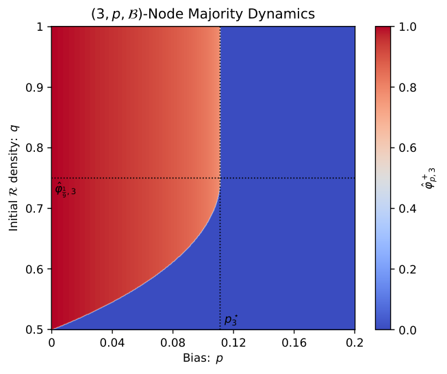
Theorem 5.4 also states that, in the slow disruption regime, after a constant number of rounds the fraction of nodes remains concentrated around a constant value greater than ; for this reason we also call such a regime metastable. From the previous description, the two dynamics appear identical. However their behavior is only qualitatively the same, given that they can differ in the critical values and in the metastable fraction of nodes in state . In fact, the critical values and do not always coincide, as described in detail in Remark 5.3 and depicted (for ) in the phase diagrams in Fig. 1.
In particular, the critical values are equal to a value whenever the initial density is larger than a threshold , for -Edge Majority, or , for -Node Majority; this happens, e.g., when starting from an initial consensus. When is smaller than such thresholds, instead, the critical values of the two dynamics become different. In this sense, when is small, the effect of the bias in the -Edge Majority is stronger than in the -Node Majority; in fact, whenever the initial density is below , there exist values of the bias such that the former dynamics is in the fast disruption regime while the latter is in the slow disruption regime. Formally, it holds that . Such phenomenon can also be observed in Fig. 1 by noting that the red area in the right diagram, representing the slow disruption regime, is larger than the red area in the left diagram.
However, as precisely stated in Theorem 5.4, the robustness of the -Majority in the two models of bias can be also measured as the fraction of nodes in state during the metastable phase, which we respectively call and . From this other point of view, the effect of bias in the -Edge Majority is weaker than in the -Node Majority. In fact, in the slow disruption regime, the concentration of nodes in the former dynamics is higher than in the latter, namely (as follows from Lemmas 4.2 and 4.5 and from Eq. 6). This phenomenon can be also observed in Fig. 1 by noting that the red area on the left diagram is more intense than that on the right diagram. We discuss applications of such a metastable behavior in Section 1.1.

We further analyze the “limit cases” of the -Majority in Section 6. When the dynamics reduces to the Voter Model; we prove that it does not exhibit any phase transition phenomenon and that, in particular, it is not robust to the external bias, resulting in a constant time of disruption for every arbitrarily small constant (see Proposition 6.1). When instead the sample is large, either in Deterministic Majority (the sample of a node deterministically coincides with its neighborhood, Definition 6.2) or when the size of the sample grows with , the dynamics exhibit again sharp phase transitions on the critical value (see Proposition 6.4 and Proposition 6.6).
Last but not least, we mention here also our analysis of the tree-processes, which let us analyze the two dynamics in a simplified topological setting where the graph is a directed infinite tree. They are presented before the other results, in Section 4, since they allow to grasp the intuitions behind the proofs without getting involved in technical details, allowing to remove some dependencies in the process. Moreover, they allow to easily understand the “duality” of the two models of bias, i.e., the fact that the concentration of in the metastable phase (slow disruption regime) is related by a linear relation (Eq. 6). In more detail, the phase transition in these models concerns the probability of the root to be in state as the number of rounds goes to infinity (Theorems 4.3 and 4.6). Roughly speaking, the tree-processes look at the local point of view of a node , showing how its state at round solely depends on the states of the nodes sampled in round ; how, in turn, the states of such nodes at round solely depend on the states of the nodes they sampled at round ; and so on until we get the dependency on the initial configuration at round .
We remark that this paper extends preliminary work already appeared in conference proceedings [CMQR20, CMQR21] where most of the technical details are omitted for lack of space. In the current version all the full proofs are included. The results are now framed in a different scenario and presented under a different point of view that allows to focus on the robustness of the -Majority dynamics w.r.t. adversarial noise, better fitting our models; the results are also extended to a new form of bias (namely -Node Majority) and described through a unified mathematical framework.
1.1 Further Applications and Research Directions
Other than directly studying the robustness to adversarial noise of the -Majority in the two forms of bias we introduced, our framework has other applications which we discuss in this section.
1.1.1 Metastability for Community Detection
The same biased communication model of the -Edge Majority has been previously used to analyze the 2-Choices on core-periphery networks [CNNS21]. The main theorems in this paper are more general (we consider -Majority for any and Deterministic Majority instead of only the 2-Choices dynamics), more comprehensive (we consider a random initialization instead of only a monochromatic one), and more precise in the description of the behavior of the dynamics (e.g., we explicitly derive the constant time in which the metastable phase is reached and quantify the concentration of nodes in state in the metastable phase). Thanks to Theorem 5.4, it is easy to extend the results of [CNNS21] also for the -Majority dynamics when .
The arise of a metastable phase makes the framework suitable to design distributed algorithms for community detection based on the -Majority dynamics, similarly to what have been done in [CNS19]. In particular, this is possible for a class of graphs known as volume-regular graphs, recently introduced in [BCPR20] and strictly related to ordinary lumpable Markov Chains [KS60]. Notable examples of volume-regular graphs are those sampled from the regular Stochastic Block Model [HLL83], where the nodes are partitioned into several clusters. As motivating example, consider a volume-regular graph where the vertex set is partitioned into two clusters . Since is volume-regular, it has the property that, for every pair of nodes in each cluster, their fraction of neighborhood toward the other cluster equals some constant . Let run the -Majority and suppose to start from an initial configuration such that the two clusters have a local majority on opposite states, say nodes in agree on and nodes in on . Such an initial configuration (in which clusters have opposite majorities) can be obtained, e.g., via a “lucky” random initialization in which each node chooses its state between and with probability and independently of the others, as shown in [CNS19]. The local evolution of such a process inside, e.g., can be described by the -Edge Majority dynamics run by the subgraph induced by : the effect of noise, with probability , mimics the fact that a node in is sampling a neighbor in in the worst-case scenario in which nodes in never change color. If is such that , then Theorem 5.4 implies that the majority in is maintained, w.h.p., for any polynomial number of rounds. Since the same reasoning, by symmetry, can be done for , it follows that the graph would stay, for any polynomial number of rounds and w.h.p., in a configuration that highlights its clustered structure for rounds.
Running the dynamics for a suitable number of (parallel) times, as shown in [CNS19, BCPR20], makes the -Majority suitable for the design of distributed community detection protocols. The results in Section 6, interestingly, show that the Voter Model cannot be used for this task because it does not exhibit a threshold behavior and especially does not exhibit any metastable phase.
1.1.2 Biased Opinion Dynamics
The -Node Majority can also be seen as a biased opinion dynamics used to model the diffusion of an inherently “superior opinion” ( in our case), e.g., modeling the introduction in the market of a new technology that will eventually substitute the status quo. The metastable behavior of the dynamics demonstrates how the density of the graph negatively affects the time needed by the superior opinion to prevail in the network.
Our model has been introduced for this very goal in [ABC+22], with the only difference related to the synchronicity of the models: while in this paper all nodes update their state simultaneously at each round, in [ABC+22] one node is selected uniformly at random at each time step to update its state. The bias, however, directly apply to the states of the nodes with a fixed probability of changing them to the superior opinion. The dynamics considered in [ABC+22] are the Deterministic Majority and the Voter Model; other than those two, herein we also analyze the -Majority dynamics.
The results in [ABC+22] show a sharp phase transition around for sufficiently dense graphs and while considering the Deterministic Majority dynamics: whenever the bias they prove a lower bound which is exponential in the minimum degree (hence, superpolynomial whenever the minimum degree is superlogarithmic); when , instead, the convergence to the superior opinion happens quickly in updates. The results drastically change while changing the underlying dynamics to the Voter Model: there is no phase transition phenomenon and the convergence to the superior opinion happens quickly in updates.
In Section 6 we analyze the same dynamics in the synchronous model, where at each time step all nodes update simultaneously. Looking at our results (Propositions 6.1 and 6.5), we note that they essentially match with those in [ABC+22]. When considering Deterministic Majority, we observe the same phase transition phenomenon on the critical value (Proposition 6.5). Regarding the slow disruption regime, while considering sufficiently dense graphs, we both get superpolynomial lower bounds in the time of disruption (or convergence of the superior opinion). Regarding the fast disruption regime, instead, we get a disruption in 2 rounds w.h.p., while in [ABC+22] updates are needed. Note that a factor is due to the different synchronicity of the models, therefore the behavior of the Deterministic Majority in the two models match up to a logarithmic factor. Moreover, both in Proposition 6.1 and in [ABC+22] no phase transition is observed when considering the Voter Model as underlying dynamics.
Herein, though, the results are also generalized for the -Majority. When considering an initial consensus configuration (i.e., ), we prove the existence of a threshold value that increases with and moves from (for ) up to (for ). The result presented in this paper could likely be proven also in the asynchronous setting studied in [ABC+22] by means of different probabilistic techniques, with the same threshold values.
1.1.3 Further Directions
It remains unclear whether it is possible to prove similar results for sparser topologies. More precisely, it would be interesting to see how our results could be sharpened by assuming a particular topology as, e.g., an Erdős–Rényi random graph with , for a constant close to the connectivity threshold.
From the statistical physics perspective, it would also be of interest the analysis of the critical case on some topologies. In particular, it would be notable if precise asymptotics on the convergence time could be obtained in the critical regime without any topological assumption on the graph.
2 Related Work
2.1 Dynamics for Consensus
Simple mathematical model of interaction between nodes in a network have been studied since the first half of the 20th century in statistical mechanics, e.g., to model interacting particle systems or ferromagnetism phenomena [Lig12]. The simplest dynamics of interaction between the nodes involve local majority-based changes of states, e.g., as in the voter model [HL+75, DW83] or in the majority dynamics [KR03]. A substantial line of research has been devoted to study the use of such simple dynamics as lightweight distributed algorithms to solve complex tasks, mirroring the behavior of complex systems from which they take inspiration. Here we are interested in discussing some of the contributions among the large body of work on dynamics for consensus. The reader is deferred to [BCN20] for a more detailed survey on the topic. All dynamics taken into consideration share a common communication model, where nodes can pull information from some fixed number of neighbors before updating their state.
The Voter Model is the first—and arguably the simplest—dynamics considered for consensus. Hassin and Peleg [HP01] proved that the dynamics reaches a consensus on state with probability proportional to the volume of nodes initially in state in rounds, regardless of the graph structure, where is the number of nodes in the network. Recently the upper bound has been improved to [KMS19], which is shown to be tight. However, the dynamics is slow in reaching consensus, e.g., it needs rounds in the complete graph despite the extremely good connectivity properties of the topology.
Therefore, simple generalizations of the Voter Model have been considered in order to achieve a faster distributed algorithm for consensus. One of the directions has been that of considering more than a single neighbor in the sample. For example, in the -Majority dynamics [BCN+17], the time needed to reach a consensus on the complete graph lowers from to [CEOR13, GL18].
The 2-Choices dynamics is a variation of the Voter Model in which nodes sample two random neighbors and update their states to the majority among two, breaking ties toward their own states. The dynamics has been studied with opinions on -regular and expander graphs [CER14], proving that, given a sufficient initial unbalance between the two opinions, a consensus on the initial majority is reached within a polylogarithmic number of rounds, with high probability. Such results have been later improved in [CER+15], relaxing the assumptions on graph’s expansion, and generalized to the case of multiple opinions [CRRS17, EFK+17]. More recently, the 2-Choices dynamics has been analyzed on networks with a core-periphery structure [CNNS21], where, depending on the initialization, it exhibits a phase transition phenomenon.
The -Majority dynamics is faster than the Voter Model in reaching consensus on well connected graphs, e.g., on the complete graph the time lowers from to [CEOR13, GL18]. On the complete graph and with possible opinions, the process converges to a plurality consensus in with high probability, if the initial unbalance between the plurality color and the second one is large enough [BCN+17]. In [BCE+17] unconditional lower and upper bounds for 2-Choices and 3-Majority on the complete graph are provided, whenever the number of initial colors is large. The scenario in which an adversary can modify some of the opinions, again for 2-Choices and/or 3-Majority, is considered in [BCN+16, DGM+11, GL18], with the best result proving convergence to a valid consensus in rounds, with high probability, even if the adversary can control nodes. The -Majority dynamics has been recently analyzed also on non complete topologies [KR19]. The authors consider a random initialization in which every node is red with probability and blue otherwise and graphs with minimum degree . Their result implies, e.g., a consensus on state red in rounds, w.h.p., if .
To the best of our knowledge, -Majority has not been extensively studied for generic . Among the few papers that consider it, in [AD15] such a dynamics (sampling without replacement) is analyzed for on the configuration model. Differently from our contribution, the paper analyzes the process on sparse graphs with low-degree sequences, namely with maximum degree that is sublinear in and the average degree that is . Similarly to our paper, the the real evolution of the dynamics on the graph is “approximated” by the dynamics on some regular trees. In particular, the analysis relies on a coupling between the real process and a process on regular trees, exploits the sparsity of the graph to ensure many local tree-like structures, and makes use of other structural properties to handle those vertices which belong to short cycles. The paper proves that the process converges to the initial majority within steps, with high probability. In [ABF15], instead, the dynamics is analyzed on preferential attachment graphs with similar convergence upper bounds to [AD15]. In [SS20] a new model is proposed, which contains majority rules as special cases. In particular, for -Majority with odd and in a binary state setting, the convergence time on expander graphs is proved to be rounds for .
The Deterministic Majority differs from the other dynamics since there is no randomness in the interaction, which is a fundamental feature of the dynamics previously discussed. This deterministic protocol has been extensively studied in the literature; we mention, for example, its analysis on expander graphs [MNT14, Zeh20], random regular graphs [GZ18], and Erdős-Rényi random graphs [BCO+16, Zeh20].
2.2 Biased Communication Models in Opinion Dynamics
A different perspective coming from other disciplines, such as economics and sociology, is that of considering interaction models between nodes of a network as models of opinion diffusion. The main models, e.g., DeGroot [DeG74] and Friedkin–Johnsen [FJ90], are based on averaging dynamics, i.e., nodes move toward the average opinion seen in their neighborhoods. Nevertheless, also the dynamics previously discussed can be framed in the modeling of opinion dynamics (see, e.g., [ABB19, AFG18, MBCD19, MT17, SLST17]).
Some opinion dynamics have been considered with biased communication models, specially in asynchronous case. The binary Deterministic Majority dynamics has been considered in a setting where nodes have a fixed private opinion and, when active, announce a public opinion as the majority opinion in their neighborhood, but ties are broken toward their private belief. Such a process has been proved to converge to the initial private majority whenever the graphs are sufficiently sparse and expansive [FILW14] or preferential attachment trees [BIMW20]. The binary Deterministic Majority dynamics, as well as the binary Voter Model, have also been analyzed in asynchronous models presenting different forms of bias [MMR16, ABC+22]. In [MMR16], if the network prefers, say, opinion instead of , every node holding opinion updates more frequently than the others; this particular feature is modeled by allowing nodes in state to revise their opinion at all points of a Poisson process with rate .
In [ABC+22, LGP22] the bias is defined toward a superior opinion: nodes have a fixed probability of updating their state to such an opinion, independently of the dynamics. The analysis in [ABC+22] is relative to the asynchronous Voter Model and Deterministic Majority dynamics. The paper proves that network density negatively affects the speed of convergence to the superior opinion when the dynamics is Deterministic Majority, while it does not play any role when the dynamics is the Voter Model. New results for sparse graphs in the same model of bias have been provided in [LGP22], proving a polynomial-time convergence to the superior opinion in cubic graphs and an exponential-time convergence to the superior opinion in sparse (constant degree) random regular graphs, for suitable values of the bias.
Another variant of bias in the Voter Model is analyzed on static and dynamic graphs (with the constrain that the degrees of the nodes do not change over time) in [BGKMT16]. There are opinions associated with popularities , so that the preferred opinion has strictly larger popularity than the others (i.e., w.l.o.g.). In each round each node samples a random neighbor and adopts its opinion with probability . On static graphs, the paper proves that, if the preferred opinion is initially supported by nodes and for some positive constant , then the process converges to a consensus on the preferred opinion with high probability within rounds, with being the conductance of the graph.
A biased version of the Voter Model has also been studied in a synchronous model in [BGKM16]: the nodes, after selecting a random neighbor, have a probability of copying its state that depends on the state itself.
In [dCN20] the binary Undecided State dynamics, a variation of the Voter Model using one extra state (the undecided one) and introduced in [AAE08], is analyzed in the complete graph in a communication model presenting a uniform noise, i.e., every state can be confused with the opposite with probability . The authors show a phase transition: if the process rapidly reaches a metastable regime of almost-consensus which lasts for polynomial time; otherwise, if , the initial majority is lost within a logarithmic number of rounds. In the same communication model with uniform noise and in the same complete topology, also the 3-Majority dynamics has been analyzed, exhibiting the same phase transition on a critical value [dZ22].
3 Preliminaries
3.1 Notation and Computational Model
Consider a sequence of graphs , where and . Note that the graphs we consider are not necessarily connected and can also be directed. We are interested in the asymptotic case in which and therefore, to simplify the notation, we will usually drop the dependence on . For the same reason, we will often use the Bachmann–Landau notation (i.e., ) to describe the limiting behavior of functions depending on .
For each node , let be the neighborhood of . In the following, we focus only on sufficiently dense graphs, i.e., graphs where every node has degree .11 1 We refer to such graphs as “sufficiently dense” in order to highlight the lower bound on the degree of the nodes that is necessary for our proof techniques. In the case of directed graphs, the restriction is on the out-degree of nodes, namely the number of outgoing directed edges.
In this paper, a dynamics on a given graph is a process that evolves in discrete, synchronous rounds,22 2 Equivalently, nodes have access to a shared clock. where, in every round , every node has a binary state that can change over time according to a function of the states of its neighbors; we denote the configuration of the system at round , i.e., the vector of states of the nodes of , as ; we define
| (1) |
We consider two different dynamics on the graph , namely the -Edge Majority dynamics (Definition 3.1) and the -Node Majority dynamics (Definition 3.2). Both processes are obtained from the -Majority dynamics by introducing a bias toward one of the two states, which we assume to be the state . Recall that in the -Majority dynamics, in each round, every node samples neighbors uniformly at random and with replacement; then it updates its state to the state held by the majority of the neighbors in the sample in the previous round; ties are broken uniformly at random. Differently, in the -Edge Majority dynamics, whenever node samples a neighbor , the state of can be seen by as with probability regardless of its actual state (as if an external agents corrupts the communication that is modeled through Z-channels [MMK03]). Instead, in the -Node Majority, whenever node updates its state, it has a probability of choosing state regardless of the actual majority in the sample, i.e., the nodes spontaneously change state to with probability (as if corrupted by an external agent).
With a slight abuse of notation we let denote both the law of the -Edge Majority and that of the -Node Majority dynamics on the graph , taking care of specifying the dynamics to which the law refers to in the rest of the paper. We use the notation for the indicator variable of the event , i.e., if holds and otherwise. Formally, -Edge Majority can be described as follows. Let be the parameter that models the bias toward state ; let be the size of the sampling. For each round , let be the multiset33 3 Recall that the sampling is with replacement. of neighbors sampled by node in round . For each sampled node , we call the state in which node sees after the effect of the bias, i.e., if , and with probability otherwise; formally
We define
| (2) |
as the sets of sampled nodes that sees respectively in state and after the effect of the bias .
Definition 3.1 (-Edge Majority dynamics).
Let and . Starting from an initial configuration , at each round every node updates its state as
Similarly, the -Node Majority can be formally defined as follows. We define
respectively as the set of neighbors in state and in state that node samples at round ; for every and every , denote by the Bernoulli random variable of parameter which models the bias toward node in round , i.e., with probability and otherwise.
Definition 3.2 (-Node Majority dynamics).
Let and . Starting from an initial configuration , at each round every node updates its state as
Note that the -Edge Majority dynamics and the -Node Majority are Markov chains, since the configuration in a round depends only on the configuration at the previous round, i.e., . Moreover, when , they both have a single absorbing state in which for every . Indeed, being the configuration space finite for every choice of , it is easy to prove that the probability of jumping to such a configuration is positive when is positive, e.g., giving a simple lower bound of to the event that all nodes see all their neighbors in state in any given round for the -Edge Majority dynamics or for the event that all neighbors directly update to state for the -Node Majority dynamics. Moreover, such a configuration is the unique absorbing state. Indeed, once such a configuration in reached, none of the nodes can change its state to at any subsequent round.
We consider initial configurations in which each node is in state , independently of the others, with probability . This choice of guarantees, by a concentration of probability argument, an initial majority of nodes in state with high probability. The two dynamics that we analyze allow to study the robustness of the -Majority when either the communication between nodes or the nodes themselves can be corrupted. In particular, both dynamics model an external, adversarial agent that tries to subvert the initial majority on state toward state . For this reason, as previously announced, we give the following definition of time of disruption .
Definition 3.3 (Time of disruption).
The time of disruption of the majority is the stopping time
In other words, the time of disruption is the first time at which the initial majority is subverted by state . Note that we fix the threshold for disruption at for the sake of simplicity, but our results hold for any constant arbitrarily close to .
In the following sections (and wherever previously used), we say that an event holds with high probability (w.h.p., in short) if . In this sense, our results only hold for large . We also use the notation to indicate a random variable sampled from the Binomial distribution of parameters (number of trials) and (probability of success).
3.2 On Even Values of the Sample Size
In the rest of the paper we assume samples of odd size , thus avoiding potential ties. In this section we show that this assumption is not restrictive. In fact, in Proposition 3.4 we prove the equivalence between the Markov chains -Edge Majority and -Edge Majority (respectively, for the Markov chains -Node Majority and -Node Majority). The result in Proposition 3.4 is essentially a special case of [FN19, Appendix B], but it has been obtained independently and with a simplified proof.
Proposition 3.4.
Let be a graph with binary state configuration in round . Fix some and and consider the -Edge Majority (-Node Majority, respectively) dynamics. For each node define the event that node is in state at round , i.e.,
Then, for every it holds
Proof.
Fix any . We first consider a single round of the -Edge Majority dynamics conditioned on the configuration at step , i.e., . In order to ease the reading we omit the explicit conditioning on in our notation. Consider the event as “Node is in state at round ”. Let us focus on samples of odd size, i.e., , where there cannot be ties. Let us define , i.e., the probability that sees a given node in the sample in state , and the random variable modeling the number of nodes seen in state out of a sample of size . Since the samples are independent, one can study the event by coupling it with the event and performing an additional sample (with as success probability) after the first . For this purpose, we also define the random variable . Therefore:
- 1.
- 2.
Moreover, note that Therefore we conclude the proof by plugging the latter equivalence into the previous formulation of , getting that .
In the case of the -Node Majority dynamics we can proceed in a similar way. Indeed, defining , we get
- 1.
- 2.
Hence we can conclude as in the previous case. ∎
Corollary 3.5.
Consider a graph with any initial configuration and fix any . For every , the -Edge Majority (-Node Majority, respectively) dynamics and the -Edge Majority (-Node Majority, respectively) dynamics follow the same law.
Proof.
By Proposition 3.4 and the independence in the updates, at each fixed round , conditioned to the configuration at round , the dynamics with and have the same law, for any integer . As a consequence, using the chain rule and the Markov property, this property can be extended for every finite set of rounds. This concludes the proof since the absorbing time is almost surely finite. ∎
4 The Tree-Processes
Consider a given node of a graph . The state of in round is a random variable which is measurable with respect to the state in round of the neighbors that samples in round , say . Similarly, the states in round of depend only on the states in round of the neighbors that they sample in round , say . Iterating this argument, we end up concluding that the state of in round depends only on the states of . Let us assume for the moment that is a collection of distinct vertices. Then, in order to sample the color of in round it is enough to consider the first layers of an infinite -regular directed tree having as a root and in the -th layer, for . On such a directed tree we consider the analogue of the -Edge Majority (respectively, -Node Majority), which is defined as follows.
Let be our -regular infinite tree with edges oriented toward the children. We call the root of . For each node we define the binary state that can change over time as described in Definition 3.1 (for the -Edge Majority) and in Definition 3.2 (for the -Node Majority), but with the only difference that will be the set of children of node . It is clear by the argument at the beginning of this section that the tree-process can be coupled with the process on the graph in a way that if the vertices are all distinct then the color of the root in round coincides with the color of the vertex in the graph at the same time.
In what follows we analyze such a tree-process and completely characterize its behavior. In the forthcoming Section 5 we show that the quantities appearing in the analysis of this process can be recovered by analyzing the expected density of vertices in state at a given time .
In order to make the exposition clearer, in what follows we separate the analysis of the tree-process for the two dynamics in separate subsections.
4.1 -Edge Majority Dynamics
As discussed in Section 3, let us define the binary random variable for each round , each vertex , and each child of . In each round we construct the sets and as described in Section 3. We study the evolution of the probability of the event “”, i.e., the root of is in state at round . The result in the forthcoming Theorem 4.3 is based on the analysis of the function , described by the following definition, that represents the evolution of the event under analysis. To ease the intuition, if at any time each vertex has probability of being in state , then the probability that a given vertex is in state at the next step is given by .
Definition 4.1 (Function ).
Let and let . Let . We define the function as
In particular, we will use the following facts about , which are proved in Appendix A and depicted in Fig. 2 (left plot).
Lemma 4.2.
For every finite odd , there exists such that:
- •
if , there exist with such that has solutions , and . Moreover, for while for ;
- •
if , there exists such that has solutions and . Moreover if ;
- •
if , then has as unique solution. Moreover, if .
Furthermore, the sequence is increasing.
Note that it is not possible to give a closed formula of for generic because it is the root of a polynomial of degree ; numerical approximations can be computed for any given . However, as proven in Lemma 4.2, monotonically increases with , starting from (for ) and up to (its limit value as , as proven in Lemma A.9).
We now prove the following theorem, which will be a guideline for the whole paper.
Theorem 4.3.
Consider the -Edge Majority dynamics on , where at round each vertex of the tree is in state with probability or in state with probability , independently of the others. Define for . Then, fixed the value of , the sequence is monotone and can be rewritten as
| (3) |
Moreover we have
| (4) |
Proof.
Define and observe that, since we are working on an infinite tree, we have for all and for all . Note also that, for any siblings , the events “” and “” are independent at any round . Hence the random variables in the family are i.i.d. and .
Let us now compute . We have:
Note that the family of random variables is independent of the family of random variables . Therefore is a family of i.i.d. Bernoulli random variables of parameter and hence
Thus, for every , we can write
| (5) |
By Definition 4.1, the sequence described in Eq. 5 can be rewritten as
Hence, the limit behavior in Eq. 4 and the monotonicity of the sequence follow from Lemma 4.2. ∎
4.2 -Node Majority Dynamics
As described in Section 3, while in -Edge Majority there is a bias in the communication channels, in -Node Majority each node can spontaneously change state to with probability . As for the other model, we study the evolution of the probability of the event “”, i.e., the root of is in state at round . The result in the forthcoming Theorem 4.6 is based on the analysis of the function , described by the following definition, that represents the evolution of the event under analysis.
Definition 4.4 (Function ).
Let and let . Let . We define the function as
Note that, since
| (6) |
the graph of the function can be obtained from the graph of the function through contractions on both the coordinate axes. See Fig. 2 (right plot) for a comparison between and .
Lemma 4.5.
For every finite odd , there exists such that:
- •
if , there exist with such that has solutions , and . Moreover, for while for ;
- •
if , there exists such that has solutions and . Moreover if ;
- •
if , then has as unique solution. Moreover if .
Furthermore, the sequence is increasing.
Note that by Eq. 6 the equation is equivalent to the equation , where . Hence the value for the -Edge Majority, introduced in Lemma 4.2, coincides with the value for the -Node Majority, introduced in Lemma 4.5.
We now prove the following theorem, which is the analogue of Theorem 4.3 for the -Node Majority.
Theorem 4.6.
Consider the -Node Majority dynamics on , where at round each vertex of the tree is in state with probability or in state with probability , independently of the others. Define for . Then, fixed the value of , the sequence is monotone and can be rewritten as
| (7) |
Moreover we have
| (8) |
Proof.
Define and observe that, as in the other model, for all and for all .
Let us now compute . Since and is odd, we have
| (9) |
Note that, for any siblings , the events “” and “” are independent at any round . Hence the random variables in the family are i.i.d. and . So we have
and hence by Eq. 9 we get
By Definition 4.4 the above sequence can be rewritten as
Hence, the limit behavior in Eq. 8 and the monotonicity of the sequence follow from Lemma 4.5. ∎
5 Phase Transition
In this section we exploit the results in Section 4 to analyze the behavior of -Edge Majority and -Node Majority on sufficiently dense graphs.
We start by setting the ground for Theorem 5.4, introducing the required notation. For every node and for every round we define the fraction of neighbors of in state as where is defined in Eq. 1. Similarly we let denote the maximum fraction of neighbors in state at round over the nodes.
Given any configuration , we have that, for every , the expected fraction of neighbors of in state at round is as follows:
- •
- •
For the -Node Majority:
(11)
Note that in Eq. 10 we have applied Definition 4.1, and used the fact that, given , we have , for every . Similarly, in Eq. 11 we have applied the definition of in Definition 4.4 and used the fact that, given , we have , for every .
Remark 5.1.
In what follows, the only features of the dynamics that will be relevant are essentially those of the functions (for the -Edge Majority) and (for the -Node Majority). As seen in Eq. 6 the graph of can be obtained from the graph of through contractions on both the coordinate axes. Hence in the rest of this section we will focus only on the -Edge Majority and all the results presented in this section can be obtained for the -Node Majority by replacing by and by , respectively.
In order to state the main result of the paper, we need the following definition.
Definition 5.2.
Fixed , and , we define as the unique solution of the optimization problem
| (12) |
where and are defined as in Lemma 4.2. Note that .
By Lemma A.7 we have that the map is increasing. Moreover, being composition of continuous functions, such a map is also continuous. Since , there exists some for which for all . Hence in Eq. 12 is well defined. Moreover is also increasing in .
Remark 5.3.
Note that, by Definition 5.2, the limit behavior of the sequence in Theorem 4.3 can be rewritten as
Defining also as the analogue of for the -Node Majority, that is
| (13) |
where is defined as in Lemma 4.5, we have that the limit behavior of the sequence in Theorem 4.6 can be rewritten as
Note that, by Eq. 6, Lemma 4.2 and Lemma 4.5, we get that and hence, by calling , we get
Moreover, the equality holds if and only if (where both take value ) or if (defined in Lemma 4.2). For the first implication it is enough to realize that if then, by the monotonicity of , we have
and by Eq. 12 and Eq. 13 it immediately follows that
For the other implication, notice that if there exists some such that
then it must be that . Moreover, since the solutions of Eq. 12 and Eq. 13 are monotonically increasing and , in order to have the equality it is necessary that is sufficiently big to imply . The conclusion follows by noting that
The main result of this work is described rigorously by the forthcoming Theorem 5.4, which shows the existence of a phase transition in the bias when the nodes of a dense graph execute -Edge Majority starting with a random configuration in which each vertex is in state independently with probability . Roughly speaking, on the one hand Theorem 5.4 states that, if the bias is smaller than the critical value , a superpolynomial number of rounds is needed to reach disruption: we will show that the system will remain trapped in a metastable phase in which the volume of nodes in state is some constant fraction of the total (larger than ) for every polynomial number of rounds. On the other hand, if the bias is larger than , a constant number of rounds w.h.p. suffices to reach disruption.
Theorem 5.4.
Fix and consider a sequence of graphs such that . For every fixed consider the -Edge Majority dynamics with odd . Assume that the system starts from an initial configuration in which each vertex is with probability , independently of the others.
- 1.
Slow disruption: if , then for all constant there exists a constant such that for all constant
where is defined as in Lemma 4.2. Hence, as a corollary, for every constant
- 2.
Fast disruption: if , then there exists a constant s.t.
(14)
Proof.
The proof for the slow disruption regime immediately follows from Corollaries 5.6 and 5.8, which are stated and proved in Section 5.1.
The proof for the fast disruption regime, instead, follows from Proposition 5.12 (by choosing ), stated and proved in Section 5.2, and from Corollary 5.6 (where ). ∎
5.1 Slow Disruption
The proof for the slow disruption regime is based on a concentration result of the density in large graph dynamics around the quantities appearing in the tree-process described in Section 4. More precisely, Propositions 5.5 and 5.7 show that for every round all the nodes in the graph have a fraction of neighbors in state which is asymptotically equal to , as defined in Eq. 3. That is to say that the tree-process is a good uniform approximation of the actual graph process for every polynomial number of rounds. We start with Proposition 5.5 which considers every starting configuration with (where is the unique point in for which , see Fig. 2). For such values of the triple we can rely on the contraction property of .
Proposition 5.5.
Proof.
Fix arbitrarily small. For all and consider the events
| (15) |
We start at by computing the probability that the event occurs, i.e.,
Fixed any , we look for a lower bound for the probability which holds uniformly in .
where in the third equality we used the fact that
and that the events and are independent for . Moreover, in the last asymptotic equality we used the classical multiplicative version of Chernoff’s bound (Theorem B.1). By the density assumption the lower bound above holds uniformly in and hence, by the union bound, we get
| (16) |
It is worth noting that up to this point we did not use the assumption on , hence Eq. 16 holds also in the case .
Now assume that the configuration is such that . Fixed any we look for a lower bound for the conditional probability , which holds uniformly in and in . We start by rewriting
Note that under any the following stochastic domination holds
Hence, called
it is sufficient to show that, for , it holds that
| (17) |
We show Eq. 17 for the case , being the proof for the case identical. By the triangle inequality and the fact that we have
| (18) |
By Lemma A.8, for all and there exists some such that
and in particular
| (19) |
Hence, by Eqs. 18 and 19, we infer
Repeating the same argument with instead of , we deduce that Eq. 17 holds. Hence, by the uniformity of the argument in and in , and by a union bound over , we get that for any
| (20) |
So by Eq. 16 and Eq. 20, for all we have
Corollary 5.6.
In the same setting of Proposition 5.5 and with the same choice of the constants, it holds
Proof.
Fix and consider assume that the configuration is such that , where is defined in Eq. 15. We have
where the symbol denotes the sum of independent variables, while the symbol denotes that the random variables in both the members of the identity have the same distribution. Notice that, by definition of we have
Therefore, by an immediate application of Hoeffding’s inequality (Theorem B.2) we get
| (21) |
In conclusion, called
and recalling the definition of in Eq. 15 and using Proposition 5.5 we deduce that, for all ,
where in the last inequality we used Eq. 21. ∎
The forthcoming Proposition 5.7 closes the gap where . Informally, Proposition 5.7 claims that within a constant number of rounds every node has at least a fraction of neighbors in state . Moreover, the fractions of neighbors in state of every vertex coincide at the first order.
Proposition 5.7.
Fix and . Consider the -Edge Majority starting from the initial configuration in which each vertex is independently of the others, with probability . If , then there exists some such that Moreover, for all constant
Proof.
We start the proof by mimicking the proof of Proposition 5.5. Consider the sequence
where
and will be defined later. For all and consider the events
We start at by computing the probability that the event occurs. Such a probability is obtained directly by Eq. 16 with instead of , i.e.,
| (22) |
As in the proof of Proposition 5.5, assume that the configuration is such that . Fixed any we look for a lower bound for the conditional probability , which holds uniformly in and in . We start by rewriting
Note that under any the following stochastic domination holds
Hence, called
it is sufficient to show that, for , it holds that
| (23) |
We show Eq. 23 for the case , with the proof for the case being identical. By the triangle inequality and the fact that we have
Therefore by the uniformity of the argument in and in , and by a union bound over , we get that for any
| (24) |
Notice that, if , by Theorem 4.3 converges to from below and hence there exists some finite
Define the sequence , where
We prove that is increasing and its increments are lower bounded by a constant uniformly in . Let us start by noting that
Hence it is sufficient to show that
| (25) |
Define
Then, we are left to show that the left hand side of Eq. 25 is strictly smaller than . This can be done by noting
and defining, for any given
In conclusion, by Eq. 22 and Eq. 24, for any we can deduce that
Using the same argument as in Corollary 5.6, we deduce the same concentration result of Proposition 5.7 for the number of vertices in state .
Corollary 5.8.
In the same setting of Proposition 5.7 and with the same choice of the constants, it holds
5.2 Fast Disruption
In the fast disruption regime, for every node of the graph, we can upper bound the expected fraction of neighbors in state . This fact is formalized by Lemma 5.9 (if ) and Lemma 5.11 (if ). In both the cases we will essentially prove that the fraction of neighbors of in state , maximized over , is a supermartingale.
Lemma 5.9.
Fix . Then there exists some such that for all , , and every configuration it holds that
Proof.
Recall the formulation, given in Eq. 10, of the expected fraction of neighbors of a node that are in state at round . Being , by Lemma 4.2, it holds for all . Moreover, the following claim holds true.
Claim 5.10.
Let . There exists a point s.t. the linear function defined as
is such that for any . Moreover, only for and , where .
Proof of 5.10.
Suppose that . Then is a convex function in . Hence
So, defining , we get the thesis in the case . Suppose now that . Imposing the equality
it is immediate that a solution is given by . On the other hand, called , the above equation reads
The latter can be rewritten as
which we know from Lemma 4.2 to have only a non-trivial solution different from zero. Called such a solution, we have that
Note that and hence, since , we have that . ∎
Lemma 5.11.
Let and consider any such that for some . Then, there exists some constant such that
Proof.
Let and consider the line
By Lemma 4.2 we have that for every . Hence, by defining
we get for every . We complete the proof of the claim by computing the conditional expectation, namely
Then, in order to conclude the proof of Eq. 14 we use the next proposition.
Proposition 5.12.
Fix . For all there exists some such that
Proof.
We divide the proof into two parts: and . We start by assuming . Consider any and fix an arbitrary . Then, by Lemma 5.9, we immediately get
| (27) |
We now aim at deriving an analogue bound as that in Eq. 27 in the alternative case in which . Start by noting that, by the definition of in Eq. 12, if it must hold . Therefore, thanks to Eq. 22 the event holds with high probability. Hence, we can apply Lemma 5.11 and conclude that Eq. 27 for every . We aim at bounding the quantity , namely
Note that, given the configuration at round , is a Binomial random variable and, thus, by applying a multiplicative form of Chernoff’s Bound (Theorem B.1), we get
Since by hypothesis and regardless of , by taking a union bound over and integrating over the conditioning we get,
| (28) |
By iterating the same argument leading to Eq. 28 we obtain that, for all ,
| (29) |
Let us call
and define the event By Eq. 29 we have . Called we get the thesis. ∎
6 Limit Cases: Voter and Deterministic Majority Dynamics
In this section we analyze the two limit cases of -Edge Majority and -Node Majority, considering the case as well as the case in which is large. In particular, -Majority is equivalent to the Voter Model, i.e., nodes copy the state of a randomly sampled neighbor. In Section 6.1 we analyze its behavior on the biased communication models described in Section 3. Notice that, in the case of the biased Voter Model, there is no difference in placing the bias on the edges or on the nodes, i.e., -Edge Majority and -Node Majority coincide. On the other hand, for large values of , one might expect the behavior of -Majority to be similar to that of Deterministic Majority, in which nodes update their state to that supported by the majority of nodes in their entire neighborhood. In Section 6.2 we investigate the relation between the two dynamics in our biased communication models.
6.1 Voter Dynamics
Differently from the general case of Theorem 5.4 where , no phase transition is observed for -Edge Majority and -Node Majority, due to the linearity of the dynamics. Moreover, the effect of the bias has a strong impact on its behavior, compared to the case . We show in Proposition 6.1 that in the biased communication model disruption is reached in rounds, w.h.p., regardless of the initial configuration and of the parameter . In other words, in a constant number of rounds any majority on state is subverted, w.h.p.
Proposition 6.1.
Fix and consider a sequence of graphs such that . For any fixed , consider the -Edge Majority (equivalently, -Node Majority) dynamics with any initial configuration . Then, there exists such that
Proof.
Recall the definition of in Eq. 2. Let us compute, for each node , an upper bound to the expected fraction of neighbors in state at round conditioned on the current configuration of states, namely
Note that, in the previous equation, the conditioning exactly determines the fraction of neighbors in state of every node at round ; thus we can compute the probability of every node to be in state in the next round. Indeed, taking into account the effect of the bias, we have
where is deterministic due to the conditioning.
As done in the proof of Proposition 5.12 for the fast convergence regime, with an application of a multiplicative form of Chernoff’s Bound (Theorem B.1) we get that
and thus a union bound over all the agents allows us to claim that
Therefore, since any initial configuration is such that , at round we have that . An application of Corollary 5.6 with implies the thesis. ∎
6.2 Deterministic Majority Dynamics
As mentioned earlier, one might expect that as grows -Edge Majority and -Node Majority would behave similarly to Deterministic Majority (where instead of sampling neighbors, nodes consider the entire neighborhood to determine their next state) in the biased communication models, which we call -edge Deterministic Majority and -Node deterministic Majority. We make this link rigorous in Propositions 6.4 and 6.6. In particular, we show that, if the graph satisfies the density assumption , both -edge Deterministic Majority and -Node deterministic Majority have a sharp phase transition at , which is in fact the limit as of the critical value (as proved in Lemma A.9). For the sake of readability, we restrict the analysis of this section to the case in which every vertex is initially in state .
Formally, the Deterministic Majority dynamics in the two biased communication models is defined as follows.
Definition 6.2 (-edge Deterministic Majority dynamics).
Let . Starting from an initial configuration , at each round every node updates its state as
where and are defined in Eq. 2 with for every .
As done in Section 3, for every and every , denote by the Bernoulli random variable of parameter which models the bias toward node in round , i.e., with probability and otherwise.
Definition 6.3 (-Node deterministic Majority dynamics).
Let . Starting from an initial configuration , at each round every node updates its state as
Proposition 6.4.
Consider a sequence of graphs such that . Fix . For any fixed , consider the -edge Deterministic Majority dynamics.
- •
Fast disruption: if , then
Hence, as a corollary,
- •
Slow disruption: if , then for all
Hence, as a corollary, for all
Proof.
Assume , for some . Notice that where are independent random variables with and
Hence, uniformly in ,
Therefore, by a union bound
Similarly, assume that , for some . Notice that where and
Hence, uniformly in ,
Therefore, by a union bound
Call the first such that , in other words,
Notice that has a geometric distribution of parameter . Hence
For every choice of independent of , we can bound
from which the claim follows. ∎
Note that the result for the -edge Deterministic Majority is much stronger than the usual disruption analysis we used throughout the paper. In fact, if for some constant , the -consensus is reached in a single round with high probability. On the other hand, if , the initial -consensus lasts for any polynomial number of rounds. We now show that -Node deterministic Majority exhibits a weaker behavior, in the sense that a fast disruption is reached in 2 rounds (instead of only 1), and in the slow disruption regime there exists a minority of nodes in state (instead, in the -edge Deterministic Majority, there are no nodes in state ).
Proposition 6.5.
Fix and consider a sequence of graphs such that . For any fixed , consider the -Node deterministic Majority dynamics.
- •
Fast disruption: if , then
Hence, as a corollary,
- •
Slow disruption: if , then, called , for all
Hence, as a corollary, for all
Proof.
The proof is in the same spirit of the one of Proposition 6.4, so we just highlight the main differences and leave the details to the interested reader. Fix . At step zero all vertices are , hence, the probability that each of them is at next step is simply given by , and those events are independent. If , after a single step w.h.p. all vertices have a fraction of neighbors which is strictly larger than , thanks to the density assumption. Therefore, conditionally on the latter event, with probability all vertices will be in state at step 2.
Concerning the scenario in which , at step 1 w.h.p. all vertices have a fraction of vertices which is larger than . Therefore, conditionally on the latter event, each vertex will be in state at the next step, independently, with probability . It is then possible to iterate the same argument for every polynomial number of rounds as in the proof of Proposition 6.4. ∎
In Proposition 6.6 we show that the -Edge Majority, for all sufficiently large values of , exhibits a behavior similar to that in Proposition 6.4. For the sake of clarity, in the next proposition we will use the notation to denote the law of -Edge Majority for a given value of . We start with the analysis of the -Edge Majority dynamics, i.e., Proposition 6.6. The corresponding results for the -Node Majority, i.e., the behavior shown in Proposition 6.7 is similar to that shown in Proposition 6.5 and can be obtained in a similar way.
Proposition 6.6.
Fix and consider a sequence of graphs such that . For any fixed , consider the -Edge Majority dynamics. For all there exists such that:
- •
Fast disruption: if , for all
(30) - •
Slow disruption: if for all and
(31)
Proof.
We first prove Eq. 30. Fix and . Assume that at round 0 all the vertices are in the state . Then
where
for some constant . Hence
where . Since , there exists such that for we have , hence . Hence applying the Chernoff’s bound (Theorem B.1) we get
uniformly in , hence Eq. 30 holds.
Let us now prove Eq. 31. Fix , and . By Lemmas A.9, 5.5 and 5.6 with , there exists such that for any fixed and for all it holds
| (32) |
Note that, since when , we have that for any there exists such that for all it holds
| (33) |
So by Eqs. 32 and 33 we get that, fixed and any , for all we have that Eq. 31 holds.
The thesis follows by choosing . ∎
We point out that the same behavior of Proposition 6.4 can be proved for -Edge Majority, by just letting grow with as .
We now state the analogue of Proposition 6.6 for the -Node Majority dynamics.
Proposition 6.7.
Fix and consider a sequence of graphs such that . For any fixed , consider the -Node Majority dynamics. For all constant there exists such that:
- •
Fast disruption: if , for all
Moreover, for all
- •
Slow disruption: if , for all and
Proof.
Also in this case the proof is similar as that of Proposition 6.6 with the same differences highlighted in the proof of Proposition 6.5. ∎
Appendix
Appendix A Properties of
Recall from Definition 4.1 that for every odd . In this section we study the fixed points of function , i.e., we want to solve the equation for every . We first consider the simplest case .
Lemma A.1.
Consider the equation . It holds that:
- •
if then there exist such that has solution , , and , with ;
- •
if then there exists such that has solution and ;
- •
if then has as unique solution.
Proof.
With we have that
With some algebraic manipulations on the equation , we get that
| (34) |
Note that Eq. 34 has solutions different from if and only if has at least one solution, i.e., if the discriminant . If then and thus the unique solution of Eq. 34 different from 0 is
If , instead, Eq. 34 has two solutions different from which are
We now look at the function for generic values of . Before stating and proving the version of Lemma A.1 for generic , we show a set of properties of the function in the following Notes A.2, A.3, A.4, A.5 and A.6
Note A.2.
Recall that . Note that:
- 1.
for every and every odd .
- 2.
for every and every odd .
- 3.
is a continuous function in the variable for every and every .
- 4.
is increasing in the variable for every and every odd . In fact, if we take , we have that
- 5.
is continuous and decreasing in for any and for every odd .
- 6.
If is odd and , we have and . In fact,
where in we use that and .
- 7.
for every and every odd . In fact, by Item 4
Claim A.3.
The function is non-decreasing in for every and , while it is non-increasing in for every and .
Proof.
Let and be two random variables with laws and , respectively. In the following we prove that
| (35) | ||||
| (36) |
Note that
Since
Eq. 37 can be rewritten as
| (37) |
Now we compute by using Eq. 37. We get that
whose sign depends only on the factor . Since if and only if , we can conclude that for every and for every .
Claim A.4.
It holds that
Proof.
We start by showing that
Observe that
| (38) |
We consider separately the term for . We have
| (39) |
Note that
| (40) |
and
| (41) |
So by Appendices A, 39, A and 41 we get
| (42) |
We want to use Appendix A for computing the derivative of . Note that
| (43) |
If we call we have that Thus, by Appendix A we can conclude that
Claim A.5.
It holds that
Proof.
We start by showing that
| (44) |
Note that
If we call we can compute the second derivative of by using Eq. 44. Indeed,
Claim A.6.
For and for any odd , the map is a convex function for .
Proof.
By direct computation:
Proof.
Recall that, by A.6, the map is convex in for all and odd. Moreover, being (Item 1 in Note A.2) and (Item 2 in Note A.2), regardless of the value of there are no solutions to the equation in the variable
as soon as . By Item 6 in Note A.2 we know that, for all odd and ,
Therefore, for all odd and there are no solutions in to the equation
since it holds
Hence, we now look for possible solutions in the interval . The case has been studied in Lemma A.1. Note that
- (i)
By A.3, the map is increasing for all and .
- (ii)
- (iii)
So, by Item i, for all there are two solutions in to the equation
By Item ii and Item iii, for all there exists a value for which the solution to the equation is unique in the interval , while for the equation has no solutions in .
Note that (see Item 2 in Note A.2) and at the beginning of the proof we have shown that has no solutions in for all odd and . Then we have that the possible solutions different from 0 of are contained in the interval .
Moreover, by Item i, we have that the sequence is increasing.
To conclude the proof we have to study the sign of . Note that, by Item 4 in Note A.2, is a continuous in the variable . Moreover, by A.6, is strictly convex in and hence
| (45) |
for all . So we conclude that for
Let us define where we assume that if . By Eq. 45, we have that . Since for and is continuous, we have that for all . This implies that
- •
if , then and hence for ;
- •
if , then and hence for ;
- •
if , then and hence for . In particular, since , then also when .
Now let us define where we assume that if . Since is continuous and , by definition of we have that for all . This implies that
- •
if , then and hence for ;
- •
if , then and hence for .
To conclude the proof we have to analyze the sign of when and . Note that if , then if . Moreover, since , then by A.6 we have that is strictly concave in . So we have
for and hence in the same interval. ∎
Lemma A.7.
The map is increasing.
Proof.
Suppose that . Then , , and are well defined (in case of , we have ). Moreover, by Item 5 in Note A.2, since , we have
| (46) |
In particular
| (47) |
Consider now the function . By Eq. 47 we have . Moreover, by Lemma 4.2, we know that
Hence, since , we have or . Suppose now that . Then, by definition of and , for any we have , that is in contradiction with Eq. 46. So it must be and hence we get the thesis. ∎
Lemma A.8.
Assume for some constant . There exists a constant such that, for all , it holds that
Proof.
In the following lemma we consider the limit of the critical bias as .
Lemma A.9.
Consider the sequence . Then we have
Proof.
Recall that
Observe that . We want to compute the limit for any . Let us define and , respectively the normalized expectation and variance of the random variable , that is
Note that
| (50) |
and by the Central Limit Theorem for the r.h.s. of Eq. 50 behaves like
| (51) |
where and is a random variable with standard normal distribution. Since
| (52) |
by Eqs. 50, 51 and 52 we get that for any
In particular for any and we have
| (53) |
By Eq. 53, for any there exists a constant such that
| (54) |
Fix and . Hence by Eq. 54 there exists a constant such that
and this implies
So we have obtained that for any there exists a constant , depending only on , such that for all . Moreover we know that is an increasing sequence bounded from above by (see Lemma 4.2). By these two facts we get the thesis. ∎
Appendix B Concentration inequalities
Theorem B.1 (Chernoff Bound [DP09]).
Let be independent random variables taking values in . Let and let . Let be such that . Then, for ,
Theorem B.2 (Hoeffding’s Inequality [DP09]).
Let be independent random variables such that . Let and let . Then, for all ,
References
- [AAE08] Dana Angluin, James Aspnes, and David Eisenstat. A simple population protocol for fast robust approximate majority. Distributed Computing, 21(2):87–102, 2008.
- [ABB19] Gideon Amir, Rangel Baldasso, and Nissan Beilin. Majority dynamics and the median process: connections, convergence and some new conjectures. arXiv preprint arXiv:1911.08613, 2019.
- [ABC+22] Aris Anagnostopoulos, Luca Becchetti, Emilio Cruciani, Francesco Pasquale, and Sara Rizzo. Biased opinion dynamics: when the devil is in the details. Inf. Sci., 593:49–63, 2022.
- [ABF15] Mohammed Amin Abdullah, Michel Bode, and Nikolaos Fountoulakis. Local majority dynamics on preferential attachment graphs. In David F. Gleich, Júlia Komjáthy, and Nelly Litvak, editors, Algorithms and Models for the Web Graph - 12th International Workshop, WAW 2015, Eindhoven, The Netherlands, December 10-11, 2015, Proceedings, volume 9479 of Lecture Notes in Computer Science, pages 95–106. Springer, 2015.
- [AD15] Mohammed Amin Abdullah and Moez Draief. Global majority consensus by local majority polling on graphs of a given degree sequence. Discret. Appl. Math., 180:1–10, 2015.
- [AFG18] Vincenzo Auletta, Diodato Ferraioli, and Gianluigi Greco. Reasoning about consensus when opinions diffuse through majority dynamics. In Jérôme Lang, editor, Proceedings of the Twenty-Seventh International Joint Conference on Artificial Intelligence, IJCAI 2018, July 13-19, 2018, Stockholm, Sweden, pages 49–55. ijcai.org, 2018.
- [BBB+22] Gregor Bankhamer, Petra Berenbrink, Felix Biermeier, Robert Elsässer, Hamed Hosseinpour, Dominik Kaaser, and Peter Kling. Fast consensus via the unconstrained undecided state dynamics. In Proceedings of the 2022 Annual ACM-SIAM Symposium on Discrete Algorithms (SODA), pages 3417–3429, 2022.
- [BCE+17] Petra Berenbrink, Andrea E. F. Clementi, Robert Elsässer, Peter Kling, Frederik Mallmann-Trenn, and Emanuele Natale. Ignore or comply?: On breaking symmetry in consensus. In Elad Michael Schiller and Alexander A. Schwarzmann, editors, Proceedings of the ACM Symposium on Principles of Distributed Computing, PODC 2017, Washington, DC, USA, July 25-27, 2017, pages 335–344. ACM, 2017.
- [BCN+16] Luca Becchetti, Andrea E. F. Clementi, Emanuele Natale, Francesco Pasquale, and Luca Trevisan. Stabilizing consensus with many opinions. In Robert Krauthgamer, editor, Proceedings of the Twenty-Seventh Annual ACM-SIAM Symposium on Discrete Algorithms, SODA 2016, Arlington, VA, USA, January 10-12, 2016, pages 620–635. SIAM, 2016.
- [BCN+17] Luca Becchetti, Andrea E. F. Clementi, Emanuele Natale, Francesco Pasquale, Riccardo Silvestri, and Luca Trevisan. Simple dynamics for plurality consensus. Distributed Computing, 30(4):293–306, 2017.
- [BCN20] Luca Becchetti, Andrea Clementi, and Emanuele Natale. Consensus dynamics: An overview. SIGACT News, 51(1):58–104, March 2020.
- [BCO+16] Itai Benjamini, Siu-On Chan, Ryan O’Donnell, Omer Tamuz, and Li-Yang Tan. Convergence, unanimity and disagreement in majority dynamics on unimodular graphs and random graphs. Stochastic Processes and their Applications, 126(9):2719–2733, 2016.
- [BCPR20] Luca Becchetti, Emilio Cruciani, Francesco Pasquale, and Sara Rizzo. Step-by-step community detection in volume-regular graphs. Theoretical Computer Science, 847:49 – 67, 2020.
- [BGKM16] Petra Berenbrink, George Giakkoupis, Anne-Marie Kermarrec, and Frederik Mallmann-Trenn. Bounds on the voter model in dynamic networks. In Ioannis Chatzigiannakis, Michael Mitzenmacher, Yuval Rabani, and Davide Sangiorgi, editors, 43rd International Colloquium on Automata, Languages, and Programming, ICALP 2016, July 11-15, 2016, Rome, Italy, volume 55 of LIPIcs, pages 146:1–146:15. Schloss Dagstuhl - Leibniz-Zentrum für Informatik, 2016.
- [BGKMT16] Petra Berenbrink, George Giakkoupis, Anne-Marie Kermarrec, and Frederik Mallmann-Trenn. Bounds on the Voter Model in Dynamic Networks. In Ioannis Chatzigiannakis, Michael Mitzenmacher, Yuval Rabani, and Davide Sangiorgi, editors, 43rd International Colloquium on Automata, Languages, and Programming (ICALP 2016), volume 55 of Leibniz International Proceedings in Informatics (LIPIcs), pages 146:1–146:15, Dagstuhl, Germany, 2016. Schloss Dagstuhl–Leibniz-Zentrum fuer Informatik.
- [BIMW20] Maryam Bahrani, Nicole Immorlica, Divyarthi Mohan, and S. Matthew Weinberg. Asynchronous majority dynamics in preferential attachment trees. In 47th International Colloquium on Automata, Languages, and Programming, ICALP 2020 (To appear), 2020.
- [BKN19] Lucas Boczkowski, Amos Korman, and Emanuele Natale. Minimizing message size in stochastic communication patterns: fast self-stabilizing protocols with 3 bits. Distributed Comput., 32(3):173–191, 2019.
- [CEOR13] Colin Cooper, Robert Elsässer, Hirotaka Ono, and Tomasz Radzik. Coalescing random walks and voting on connected graphs. SIAM J. Discrete Math., 27(4):1748–1758, 2013.
- [CER14] Colin Cooper, Robert Elsässer, and Tomasz Radzik. The power of two choices in distributed voting. In Javier Esparza, Pierre Fraigniaud, Thore Husfeldt, and Elias Koutsoupias, editors, Automata, Languages, and Programming - 41st International Colloquium, ICALP 2014, Copenhagen, Denmark, July 8-11, 2014, Proceedings, Part II, volume 8573 of Lecture Notes in Computer Science, pages 435–446. Springer, 2014.
- [CER+15] Colin Cooper, Robert Elsässer, Tomasz Radzik, Nicolas Rivera, and Takeharu Shiraga. Fast consensus for voting on general expander graphs. In Yoram Moses, editor, Distributed Computing - 29th International Symposium, DISC 2015, Tokyo, Japan, October 7-9, 2015, Proceedings, volume 9363 of Lecture Notes in Computer Science, pages 248–262. Springer, 2015.
- [CGG+18] Andrea E. F. Clementi, Mohsen Ghaffari, Luciano Gualà, Emanuele Natale, Francesco Pasquale, and Giacomo Scornavacca. A tight analysis of the parallel undecided-state dynamics with two colors. In Igor Potapov, Paul G. Spirakis, and James Worrell, editors, 43rd International Symposium on Mathematical Foundations of Computer Science, MFCS 2018, August 27-31, 2018, Liverpool, UK, volume 117 of LIPIcs, pages 28:1–28:15. Schloss Dagstuhl - Leibniz-Zentrum fuer Informatik, 2018.
- [CMPS09] Claudio Castellano, Miguel A Muñoz, and Romualdo Pastor-Satorras. Nonlinear q-voter model. Physical Review E, 80(4):041129, 2009.
- [CMQR20] Emilio Cruciani, Hlafo Alfie Mimun, Matteo Quattropani, and Sara Rizzo. Brief announcement: Phase transitions of the k-majority dynamics in a biased communication model. In Hagit Attiya, editor, 34th International Symposium on Distributed Computing, DISC 2020, October 12-16, 2020, Virtual Conference, volume 179 of LIPIcs, pages 42:1–42:3. Schloss Dagstuhl - Leibniz-Zentrum für Informatik, 2020.
- [CMQR21] Emilio Cruciani, Hlafo Alfie Mimun, Matteo Quattropani, and Sara Rizzo. Phase transitions of the k-majority dynamics in a biased communication model. In ICDCN ’21: International Conference on Distributed Computing and Networking, Virtual Event, Nara, Japan, January 5-8, 2021, pages 146–155. ACM, 2021.
- [CNNS21] Emilio Cruciani, Emanuele Natale, André Nusser, and Giacomo Scornavacca. Phase transition of the 2-choices dynamics on core-periphery networks. Distributed Comput., 34(3):207–225, 2021.
- [CNS19] Emilio Cruciani, Emanuele Natale, and Giacomo Scornavacca. Distributed community detection via metastability of the 2-choices dynamics. In The Thirty-Third AAAI Conference on Artificial Intelligence, AAAI 2019, Honolulu, Hawaii, USA, January 27 - February 1, 2019, pages 6046–6053. AAAI Press, 2019.
- [CRRS17] Colin Cooper, Tomasz Radzik, Nicolas Rivera, and Takeharu Shiraga. Fast plurality consensus in regular expanders. In Andréa W. Richa, editor, 31st International Symposium on Distributed Computing, DISC 2017, October 16-20, 2017, Vienna, Austria, volume 91 of LIPIcs, pages 13:1–13:16. Schloss Dagstuhl - Leibniz-Zentrum fuer Informatik, 2017.
- [dCN20] Francesco d’Amore, Andrea E. F. Clementi, and Emanuele Natale. Phase transition of a non-linear opinion dynamics with noisy interactions - (extended abstract). In Andrea Werneck Richa and Christian Scheideler, editors, Structural Information and Communication Complexity - 27th International Colloquium, SIROCCO 2020, Paderborn, Germany, June 29 - July 1, 2020, Proceedings, volume 12156 of Lecture Notes in Computer Science, pages 255–272. Springer, 2020.
- [DeG74] Morris H DeGroot. Reaching a consensus. Journal of the American Statistical Association, 69(345):118–121, 1974.
- [DGM+11] Benjamin Doerr, Leslie Ann Goldberg, Lorenz Minder, Thomas Sauerwald, and Christian Scheideler. Stabilizing consensus with the power of two choices. In Rajmohan Rajaraman and Friedhelm Meyer auf der Heide, editors, SPAA 2011: Proceedings of the 23rd Annual ACM Symposium on Parallelism in Algorithms and Architectures, San Jose, CA, USA, June 4-6, 2011 (Co-located with FCRC 2011), pages 149–158. ACM, 2011.
- [DP09] Devdatt P Dubhashi and Alessandro Panconesi. Concentration of measure for the analysis of randomized algorithms. Cambridge University Press, 2009.
- [DW83] Peter Donnelly and Dominic Welsh. Finite particle systems and infection models. In Mathematical Proceedings of the Cambridge Philosophical Society, volume 94, pages 167–182, 1983.
- [dZ22] Francesco d’Amore and Isabella Ziccardi. Phase transition of the 3-majority dynamics with uniform communication noise. In Structural Information and Communication Complexity: 29th International Colloquium, SIROCCO 2022, Paderborn, Germany, June 27–29, 2022, Proceedings, page 98–115, Berlin, Heidelberg, 2022. Springer-Verlag.
- [EFK+17] Robert Elsässer, Tom Friedetzky, Dominik Kaaser, Frederik Mallmann-Trenn, and Horst Trinker. Brief announcement: Rapid asynchronous plurality consensus. In Elad Michael Schiller and Alexander A. Schwarzmann, editors, Proceedings of the ACM Symposium on Principles of Distributed Computing, PODC 2017, Washington, DC, USA, July 25-27, 2017, pages 363–365. ACM, 2017.
- [FHK17] Ofer Feinerman, Bernhard Haeupler, and Amos Korman. Breathe before speaking: efficient information dissemination despite noisy, limited and anonymous communication. Distributed Comput., 30(5):339–355, 2017.
- [FILW14] Michal Feldman, Nicole Immorlica, Brendan Lucier, and S. Matthew Weinberg. Reaching consensus via non-bayesian asynchronous learning in social networks. In Klaus Jansen, José D. P. Rolim, Nikhil R. Devanur, and Cristopher Moore, editors, Approximation, Randomization, and Combinatorial Optimization. Algorithms and Techniques, APPROX/RANDOM 2014, September 4-6, 2014, Barcelona, Spain, volume 28 of LIPIcs, pages 192–208. Schloss Dagstuhl - Leibniz-Zentrum für Informatik, 2014.
- [FJ90] Noah E Friedkin and Eugene C Johnsen. Social influence and opinions. Journal of Mathematical Sociology, 15(3-4):193–206, 1990.
- [FN19] Pierre Fraigniaud and Emanuele Natale. Noisy rumor spreading and plurality consensus. Distributed Computing, 32(4):257–276, 2019.
- [GL18] Mohsen Ghaffari and Johannes Lengler. Nearly-tight analysis for 2-choice and 3-majority consensus dynamics. In Calvin Newport and Idit Keidar, editors, Proceedings of the 2018 ACM Symposium on Principles of Distributed Computing, PODC 2018, Egham, United Kingdom, July 23-27, 2018, pages 305–313. ACM, 2018.
- [GZ18] Bernd Gärtner and Ahad N. Zehmakan. Majority model on random regular graphs. In Michael A. Bender, Martin Farach-Colton, and Miguel A. Mosteiro, editors, LATIN 2018: Theoretical Informatics - 13th Latin American Symposium, Buenos Aires, Argentina, April 16-19, 2018, Proceedings, volume 10807 of Lecture Notes in Computer Science, pages 572–583. Springer, 2018.
- [HL+75] Richard A Holley, Thomas M Liggett, et al. Ergodic theorems for weakly interacting infinite systems and the voter model. The annals of probability, 3(4):643–663, 1975.
- [HLL83] Paul W Holland, Kathryn Blackmond Laskey, and Samuel Leinhardt. Stochastic blockmodels: First steps. Social networks, 5(2):109–137, 1983.
- [HP01] Yehuda Hassin and David Peleg. Distributed probabilistic polling and applications to proportionate agreement. Inf. Comput., 171(2):248–268, 2001.
- [KMS19] Varun Kanade, Frederik Mallmann-Trenn, and Thomas Sauerwald. On coalescence time in graphs: When is coalescing as fast as meeting?: Extended abstract. In Timothy M. Chan, editor, Proceedings of the Thirtieth Annual ACM-SIAM Symposium on Discrete Algorithms, SODA 2019, San Diego, California, USA, January 6-9, 2019, pages 956–965. SIAM, 2019.
- [KR03] Paul L Krapivsky and Sidney Redner. Dynamics of majority rule in two-state interacting spin systems. Physical Review Letters, 90(23):238701, 2003.
- [KR19] Nan Kang and Nicolás Rivera. Best-of-three voting on dense graphs. In The 31st ACM Symposium on Parallelism in Algorithms and Architectures, SPAA ’19, page 115–121, New York, NY, USA, 2019. Association for Computing Machinery.
- [KS60] John G. Kemeny and J. Laurie Snell. Finite Markov chains. D. van Nostrand Company, inc., Princeton, N.J., 1960.
- [LGP22] Hicham Lesfari, Frédéric Giroire, and Stéphane Pérennes. Biased majority opinion dynamics: Exploiting graph -domination. In IJCAI 2022-International Joint Conference on Artificial Intelligence, 2022.
- [Lig12] Thomas Milton Liggett. Interacting particle systems, volume 276. Springer Science & Business Media, 2012.
- [MBCD19] Wenjun Mei, Francesco Bullo, Ge Chen, and Florian Dörfler. Occam’s razor in opinion dynamics: The weighted-median influence process. CoRR, abs/1909.06474, 2019.
- [MMK03] David JC MacKay and David JC Mac Kay. Information theory, inference and learning algorithms. Cambridge university press, 2003.
- [MMR16] A. Mukhopadhyay, R. R. Mazumdar, and R. Roy. Binary opinion dynamics with biased agents and agents with different degrees of stubbornness. In International Teletraffic Congress, volume 01, pages 261–269, 2016.
- [MNT14] Elchanan Mossel, Joe Neeman, and Omer Tamuz. Majority dynamics and aggregation of information in social networks. Autonomous Agents and Multi-Agent Systems, 28(3):408–429, 2014.
- [MT17] Elchanan Mossel and Omer Tamuz. Opinion exchange dynamics. Probab. Surveys, 14:155–204, 2017.
- [PKS16] Radia Perlman, Charlie Kaufman, and Mike Speciner. Network security: private communication in a public world. Pearson Education India, 2016.
- [SLST17] Alina Sîrbu, Vittorio Loreto, Vito D. P. Servedio, and Francesca Tria. Opinion dynamics: Models, extensions and external effects. In Vittorio Loreto, Muki Haklay, Andreas Hotho, Vito D. P. Servedio, Gerd Stumme, Jan Theunis, and Francesca Tria, editors, Participatory Sensing, Opinions and Collective Awareness, Understanding Complex Systems, pages 363–401. Springer, 2017.
- [SS20] Nobutaka Shimizu and Takeharu Shiraga. Quasi-majority functional voting on expander graphs. In Artur Czumaj, Anuj Dawar, and Emanuela Merelli, editors, 47th International Colloquium on Automata, Languages, and Programming, ICALP 2020, July 8-11, 2020, Saarbrücken, Germany (Virtual Conference), volume 168 of LIPIcs, pages 97:1–97:19. Schloss Dagstuhl - Leibniz-Zentrum für Informatik, 2020.
- [Zeh20] Ahad N. Zehmakan. Opinion forming in erdős-rényi random graph and expanders. Discret. Appl. Math., 277:280–290, 2020.