Computation of free boundary minimal surfaces
via extremal Steklov eigenvalue problems
Abstract.
Recently Fraser and Schoen showed that the solution of a certain extremal Steklov eigenvalue problem on a compact surface with boundary can be used to generate a free boundary minimal surface, i.e., a surface contained in the ball that has (i) zero mean curvature and (ii) meets the boundary of the ball orthogonally (doi:10.1007/s00222-015-0604-x). In this paper, we develop numerical methods that use this connection to realize free boundary minimal surfaces. Namely, on a compact surface, , with genus and boundary components, we maximize over a class of smooth metrics, , where is the -th nonzero Steklov eigenvalue and is the length of . Our numerical method involves (i) using conformal uniformization of multiply connected domains to avoid explicit parameterization for the class of metrics, (ii) accurately solving a boundary-weighted Steklov eigenvalue problem in multi-connected domains, and (iii) developing gradient-based optimization methods for this non-smooth eigenvalue optimization problem. For genus and boundary components, we numerically solve the extremal Steklov problem for the first eigenvalue. The corresponding eigenfunctions generate a free boundary minimal surface, which we display in striking images. For higher eigenvalues, numerical evidence suggests that the maximizers are degenerate, but we compute local maximizers for the second and third eigenvalues with boundary components and for the third and fifth eigenvalues with boundary components.
Key words and phrases:
Steklov eigenvalue; eigenvalue optimization; free boundary minimal surface2010 Mathematics Subject Classification
35P05, 35P15, 49Q05, 65N25.1. Introduction
Recently, A. Fraser and R. Schoen discovered a rather surprising connection between an extremal Steklov eigenvalue problem and the problem of generating free boundary minimal surfaces in the Euclidean ball [FS11, FS13, FS15]. These findings have been further developed [FTY14, FS19, GL20] and were recently reviewed in [Li19]. In this paper, we develop numerical methods to further investigate this connection. We first briefly review some of these previous results before stating the contributions of the present work.
The extremal Steklov eigenvalue problem
Let be a smooth, compact, connected Riemannian surface with nonempty boundary, . The Steklov eigenproblem on is given by
| (1a) | ||||||
| (1b) | ||||||
where is the Laplace-Beltrami operator and is the outward normal derivative. The Steklov spectrum is discrete and we enumerate the eigenvalues, counting multiplicity, in increasing order
The Steklov spectrum coincides with the spectrum of the Dirichlet-to-Neumann operator , given by the formula , where denotes the unique harmonic extension of to . The restriction of the Steklov eigenfunctions to the boundary, , form a complete orthonormal basis of . A recent survey on Steklov eigenvalues can be found in [GP17].
Here, for fixed surface with genus and boundary components, we consider the dependence of the -th Steklov eigenvalues on the metric, i.e., the mapping . It is known that for any smooth Riemannian metric , we have the following upper bound on the -th Steklov eigenvalue in terms of the topological invariants and ,
| (2) |
Here, is the length of with respect to the metric . This bound was proven by Weinstock [Wei54] for , , and ; by Fraser and Schoen [FS11] for (see also [GP12]); and in generality by Karpukhin [Kar17]. It is then natural to pose the extremal Steklov eigenvalue problem,
| (3) |
where varies over the class of smooth Riemannian metrics on . The existence of a smooth maximizer in (3) was established in [FS15, Theorem 1.1] for oriented surfaces of genus with boundary components or a Möbius band and in [MP20] for general surfaces for the first () eigenvalue.
Free boundary minimal surfaces
Denote the closed -dimensional Euclidean unit ball by and the -dimensional unit sphere by . Let be a -dimensional submanifold with boundary . We say that is a free boundary minimal submanifold in the unit ball if
- (i)
has zero mean curvature and
- (ii)
meets orthogonally along .
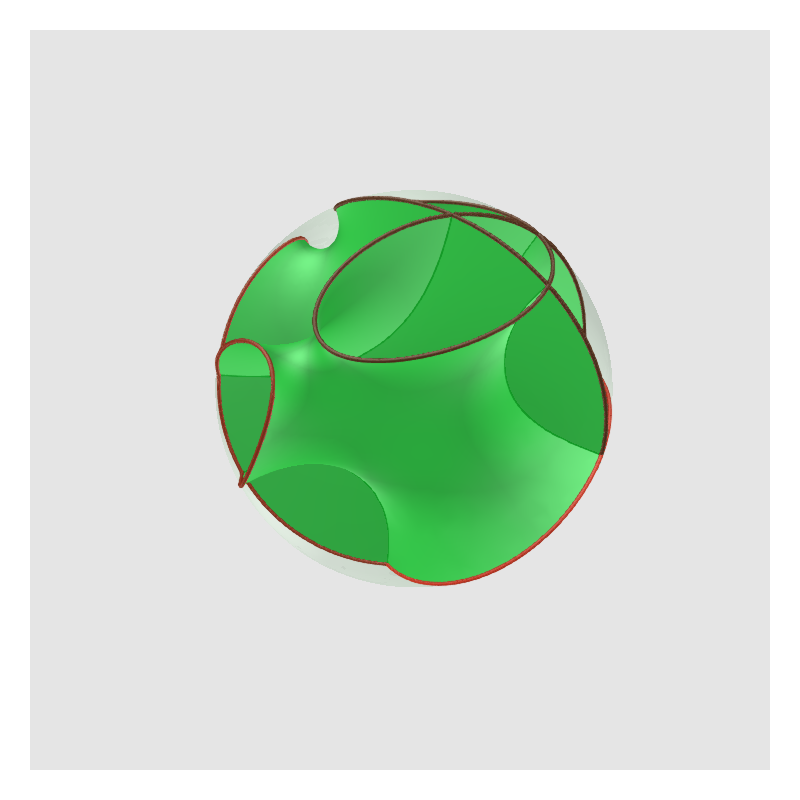
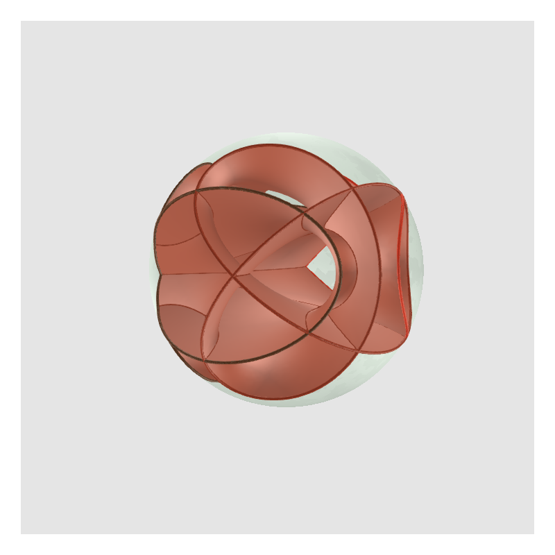
When , we call a free boundary minimal surface in the unit ball or, more simply, a free boundary minimal surface. For a good visual aid to understanding the definition of free boundary minimal surfaces (and a peak at the results of this paper), we recommend the reader take a look at the free boundary minimal surfaces displayed in Figures 13 and 14.
Fraser and Schoen’s connection
Fraser and Schoen observed that a -dimensional submanifold with boundary is a free boundary minimal surface if and only if the coordinate functions , restricted to are Steklov eigenfunctions with eigenvalue . Furthermore, they showed the following theorem.
Theorem 1.1 ([FS13]).
Let be a compact surface with boundary. Suppose that is a smooth metric on attaining the supremum in (3) for some . Let be the -dimensional eigenspace corresponding to . Then, there exist independent Steklov eigenfunctions which give a (possibly branched) conformal immersion such that is a free boundary minimal surface in and, up to rescaling of the metric, is an isometry on .
Theorem 1.1 gives a method for using the solution of (3) to compute free boundary minimal surfaces. The simplest such example is the equatorial disk, obtained as the intersection of with any two-dimensional subspace of . This can be constructed from Weinstock’s result that inequality in (2) with , , and is attained only by the round disk, [Wei54]. In this case, for the eigenvalue , we have the two-dimensional eigenspace given by . The equatorial disk is given as the map , defined by .
For genus and boundary components, the extremal metric is rotationally invariant and the corresponding free boundary minimal surface is the critical catenoid. We will discuss this example further in Section 3. For genus and boundary components, the extremal metric is not known explicitly, but it is known that the corresponding free boundary minimal surface is embedded in and star-shaped with respect to the origin [FS13]. In [GL20], the authors used homogenization methods to construct surfaces that have large first Steklov eigenvalue . In particular, free boundary minimal surfaces of genus with particular symmetries (e.g., symmetries of platonic solids) were constructed numerically. The authors proved that the first nonzero Steklov eigenvalue, , of these surfaces is and emphasized that it is not known whether these surfaces have extremal first eigenvalues among all surfaces with the same genus and number of boundary components. We will compare our results to these surfaces in Section 5.
In [FTY14], Fan, Tam, and Yu extended the study of (3) to higher values of on the cylinder (, ) among rotationally symmetric conformal metrics. They obtained different results for even and odd eigenvalues. They showed that the maximum of the , among all rotationally symmetric conformal metrics on the cylinder is achieved by the -fold covering of the critical catenoid immersed in . The maximum of is not attained. The maximum of the for among all rotationally symmetric conformal metrics on the cylinder is achieved by the -fold covering of the critical Möbius band. These results will be further discussed in Section 3 and further compared to our computed surfaces in Section 5.
Results and outline
In this paper, we develop computational methods for solving the extremal Steklov eigenvalue problem (3) and thus generating free boundary minimal surfaces via Theorem 1.1. This approach is used to realize free boundary minimal surfaces beyond the known examples of equatorial disks, the critical catenoid, the critical Möbius band, and their higher coverings discussed above.
In Section 2, we explain how the conformal uniformization of multiply connected domains can be used to significantly reduce the complexity of the general Steklov eigenproblem (1) and extremal Steklov eigenproblem (3). The argument relies on two ingredients:
- (1)
The uniformization result that for a smooth, compact, connected, genus-zero Riemannian surface with boundary components, , there exists a conformal mapping , where is a disk with holes and is a conformally flat metric.
- (2)
The composition of a function with a conformal map is harmonic if and only if is harmonic.
Let be the unit disk and
be a punctured unit disk with holes,
This argument implies that it is sufficient to consider the family of (flat!) Steklov eigenproblems,
| (4a) | ||||||
| (4b) | ||||||
where is the Laplacian on , is the outward normal derivative, and is a density function. The extremal Steklov eigenvalue problem (3) for genus is transformed to
| (5a) | ||||||
| (5b) | s.t. | |||||
| (5c) | ||||||
| (5d) | ||||||
Here, , is the -th nontrivial eigenvalue satisfying (4), and is the total length of . The first two constraints simply state that the holes are contained in the domain and are pairwise disjoint.
In Section 3, we explicitly solve the Steklov eigenvalue problem on a rotationally symmetric annulus (i.e., , , , and constant on each boundary component) and describe the critical catenoid and its higher coverings in detail. These Steklov eigenvalues and corresponding free boundary minimal surfaces will be used to verify our computational methods.
In Section 4, we develop numerical methods for computing Steklov eigenvalues satisfying (4) on multiply connected domains, computing the solution to the optimization problem (5), and the computation of free boundary minimal surfaces from the Steklov eigenfunctions. In brief, we use the method of particular solutions to compute Steklov eigenvalues, gradient-based interior point methods for the optimization problem, and compute the mapping to a surface by minimizing a particular energy. These methods build on previous computational methods for extremal eigenvalue problems on Euclidean domains, including minimizing Laplace-Dirichlet eigenvalues over Euclidean domains of fixed volume or perimeter [Oud04, Ost10, AF12, OK13, OK14, AO17, BBG17], maximizing Steklov eigenvalues over two-dimensional Euclidean domains of fixed volume [AKO17, BBG17]. These methods have recently been extended to more general geometric settings. In particular, [KLO17] maximized Laplace-Beltrami eigenvalues over conformal classes of metrics with fixed volume and compact Riemannian surfaces of fixed genus (, 1) and volume.
In Section 5, we present the results of numerous computations. For genus and boundary components, we numerically solve the extremal Steklov problem (5) for the first eigenvalue. We include figures displaying the optimal punctured disks and three linearly-independent eigenfunctions associated to the first eigenvalue, as well as tabulate the values of the obtained Steklov eigenvalues. We also plot the associated free boundary minimal surfaces, which are visually striking. Finally, in Section 5, we also present results for maximizing higher eigenvalues. Here, numerical evidence suggests that the maximizers are degenerate, but we compute local maximizers for the second and third eigenvalues with boundary components and for the third and fifth eigenvalues with boundary components. For brevity, we were only able to report the results for selected values of and ; the results of additional computations can be found on É. Oudet’s website [Oud20], along with gifs.
We conclude in Section 6 with a discussion.
2. The Euclidean Steklov eigenproblem
In Section 2.1, we explain how the conformal uniformization of multiply connected domains can be used to significantly reduce the complexity of the general Steklov eigenproblem (1) and extremal Steklov eigenvalue problem (3) to obtain the Euclidean Steklov eigenproblem and (4) and extremal Steklov eigenvalue problem (5), respectively. In Section 2.2, we also compute the eigenvalue derivatives with respect to the density and shape parameters and discuss optimality conditions for the extremal Steklov eigenvalue problem (5).
2.1. Conformal uniformization of multiply-connected surfaces and the Steklov eigenproblem
The uniformization theorem for compact, genus-zero Riemann surface without boundary states that such surfaces can be conformally mapped to the Riemann sphere. Here, we use a generalization of this result for multiply-connected surfaces; see [Hen86, Theorem 17.1b], [GL99], [ZYZ+09], and [JGHW18, p.123].
Theorem 2.1 ([GL99]).
Suppose is a smooth, compact, connected, genus-zero Riemann surface with boundary components. Then can be conformally mapped to a unit disk with circular holes. That is, there exists a punctured unit disk with holes, , and a conformal map , where is a conformally flat metric. Furthermore, two such mappings differ by a Möbius transformation.
Remark 2.2.
The uniqueness of the conformal map up to a Möbius transformation means that it is possible to center one of the holes at the origin and center another hole on the positive -axis. Thus, fixing these three parameters, the dimension of the parameter space of hole centers and radii , is 1 for and for , which is the dimension of the conformal module.
We now sketch a brief derivation of (4) from (1). Let be a conformal mapping. It is well-known that is harmonic if and only if is harmonic [Olv17]. This justifies (4a). We show (4b) on a flat domain for simplicity. Write and , so that . Since , we have that
So, we obtain , where , where .
Remark 2.2 shows that our parameterization of is over-complete, as the following example further demonstrates.
Example 2.3.
Denote as an eccentric annulus with boundaries
and as an concentric annulus where , , are real numbers and . A conformal mapping is given by
where and are determined by mapping to and satisfy
In this example, , and
In Figure 1, the mapping is shown for and the resulting .
Thus, the eccentric annulus with boundary density has the same Steklov spectrum as the concentric annulus with boundary density given above. In particular, this example shows that the decomposition of perturbations of a metric into conformal and non-conformal directions is not equivalent to either changing or , respectively. While changing is a conformal perturbation, a change in gives a perturbation to the metric that has components in both the conformal and non-conformal directions.

The following two examples illustrate what happens to the boundary density when becomes “pinched”.
Example 2.4.
We consider the conformal mapping from the unit disk to the Hippopede domain, ,
see [GLS16, AK19]. When , this is the identity mapping on the unit disk and as , it maps a unit disk to two “kissing” disks. In the left and center panels of Figure 2, the mapping is shown for . Here, we compute,
Let . In the right panel of Figure 2, we plot for , , and . We observe that becomes singular as at and .

In Example 2.4, the density is singular at two points. The following example illustrates how the density function can become singular at a single point.
Example 2.5.
We consider a radius disk, , (see Figure 3(c)) and a domain consisting of the union of two disks with radii and and a ‘neck’ of width (see Figure 3(a)). Define the conformal mapping as the composition of the two functions , where
The constants are chosen as
so that maps to , respectively. See Figure 3(a) and (b). The constant is chosen so that maps to a unit disk and the zero in maps to See Figure 3(b) and (c).When is small, this function maps points which are uniformly distributed on to points that accumulate near on the unit disk. The boundary density, , can be obtained via the product rule,
As shown in Figures 3(d), the density reaches a large value at . Figure 3(e) shows the detail profile of the density function about one.


2.2. Eigenvalue derivatives with respect to the density and shape parameters
In this section, we consider and as a function of and the shape . We first compute the derivatives with respect to .
Proposition 2.6.
Let be a simple Steklov eigenpair, satisfying (4), normalized so that . Then the functionals and are Frechét differentiable with derivatives
| (6a) | ||||
| (6b) | ||||
Proof.
We take variations of the formula and use Green’s identity to obtain
From the normalization condition, , we obtain
which gives the desired result. The derivative of is obtained via and the product rule. ∎
We describe below optimality conditions when the multiplicity of the optimized eigenvalue is greater than one. Our formulation is highly inspired by previous articles [ESI+07, FS15, BO16]. We first need the following regularity result; see [LP15, Theorem 3.2].
Lemma 2.7.
Let be an eigenvalue of multiplicity of system (4) associated to a smooth domain with nonnegative boundary density . Let and consider the eigenvalues associated to the densities for . There exists and nontrivial functions and analytic on such that for all :
- (a)
,
- (b)
The family is orthonormal in ,
- (c)
Every couple is solution of system (4) for the density .
We can now evaluate directional derivatives based on previous parametrizations:
Lemma 2.8.
Let be an eigenvalue of multiplicity of the weighted Steklov system (4) for some nonnegative boundary density . Denote by the corresponding eigenspace. Let be a perturbation of for some . Let and be some smooth parametrizations as the ones given by Lemma 2.7. Then are the eigenvalues of the quadratic form defined on by
Moreover, the -orthonormal basis diagonalizes on .
Proof.
Let and defined on for some satisfying properties of Lemma 2.7. For all , and , we have from (4), that
| (7) |
Differentiationg this equality with respect to and evaluating at gives
Thus, with and using (7) replacing per and by , we obtain
which exactly proves that -orthonormal basis diagonalizes on . Moreover, the are eigenvalues of this quadratic form. ∎
We can now establish optimality conditions with respect to the boundary density in case of multiple eigenvalues.
Proposition 2.9.
Let and a smooth domain of . Assume a nonnegative maximizes the product among all nonnegative functions of where and is the -th eigenvalues of system (4). If is of multiplicity and its eigenspace, there exists a basis of functions of which satisfy
for all .
Proof.
The proposition is an almost direct consequence of Lemma 2.8 and of Hahn-Banach separation theorem. Consider the convex hull . We want to prove that the function identically equal to one belongs to . If it is not the case, by Hahn-Banach theorem applied to the finite dimensional normed vector subspace of spanned by and , there exists a function such that and which satisfies, for all ,
This last inequality asserts that the quadratic form on has nonnegative eigenvalues. Thus, both the eigenvalues and the weighted length increase in the direction of . As a consequence, for small enough, the product of is strictly greater than due to the strict inequality of the separation result which contradicts the optimality. ∎
To compute the derivatives of and with respect to the centers and radii , we first compute the shape derivative with respect to perturbations of the boundary of . This result extends a result in [DKL14, AKO17, BBG17] to .
Proposition 2.10.
Consider the perturbation . Then a simple (unit-normalized) Steklov eigenpair satisfies the perturbation formula
| (8) |
where is the outward unit normal vector, denotes the tangential direction, and where is the signed curvature of the boundary. We also have .
Proof.
We follow the proof in [AKO17]. Let primes denote the shape derivative. From the identity , we compute
| (9a) | (shape derivative) | |||||
| (9b) | (Green’s identity) | |||||
| (9c) | ||||||
Differentiating the normalization equation, , we have that
where is the curvature of the boundary and . Extending constantly in the normal direction, we have where denotes the tangential direction. We then have that
Combining this with (9), we obtain the desired result. ∎
Using Proposition 2.10, we can now compute the derivatives of and for the domain with respect to a center and radius of as follows. To compute the derivative with respect to , we choose a perturbation so that
Then, noting that , we obtain
| (10) |
To compute the derivative with respect to , we take two perturbations of the form
and
to obtain
| (11) |
Remark 2.11.
In [FS15], a detailed study of perturbations to the metric yield two conditions for a maximal Steklov eigenvalue. The first comes from the study of perturbations in “conformal directions” and, as in Proposition 2.9, result in the existence of eigenfunctions such that the map satisfies . The second condition comes from the study of non-conformal perturbations of the metric and give that the map has isothermal coordinates, i.e., satisfies
Since a change in the parameters gives a perturbation to the metric that has components in both the conformal and non-conformal directions (see Remark 2.2 and Example 2.3), this second condition is nontrivial to obtain from (10) and (11).
3. Steklov eigenvalues of rotationally symmetric annuli and the critical catenoid
Here, we discuss the Steklov eigenvalues of rotationally symmetric annuli, the critical catenoid, and coverings of the critical catenoid. These results are also discussed in [FS11, FTY14] using cylindrical coordinates, but it useful to review these computations and have them written in annular coordinates for comparison and discussion; see also [Mar14, Dit04].
3.1. Steklov eigenvalues of rotationally symmetric annuli
Here, for , we consider the rotationally symmetric annulus,
and explicitly compute Steklov eigenvalues satisfying
| (12a) | ||||||
| (12b) | ||||||
| (12c) | ||||||
Note that if is an eigenpair satisfying (12) with parameters , then for , is an eigenpair satisfying (12) with parameters . Using separation of variables, we obtain general solutions to the Laplace equation of the form
where are constants. Using the Steklov boundary conditions, we can determine the eigenpairs, . Of course, there is a trivial eigenvalue, with corresponding constant eigenfunction. There is another eigenpair with eigenfunction that is constant in , given by
We note that , so that
For each , there are also eigenfunctions that are oscillatory in of the form
where , are constants. Here, the brackets indicate that we can choose either or ; the corresponding eigenvalue has multiplicity two. Using the boundary conditions we obtain the generalized eigenproblem,
This is equivalent to the eigenproblem
from which one obtains the real positive eigenvalues
In Figure 4(left), for , we display the length-normalized Steklov eigenvalues for various values of . The eigenvalue corresponding to the radially symmetric eigenfunction is plotted in red. The thin vertical line indicates the value . For this value of , the first Steklov eigenvalue has multiplicity three and length-normalized eigenvalue . In Figure 4(right), we plot contours of two of the eigenfunctions; the third can be obtained by rotating the image of the lower eigenfunction by .


3.2. Extremal eigenvalues for rotationally symmetric annuli
We consider the extremal eigenvalue problem for rotationally symmetric annuli,
| (13) |
Here, is assumed to satisfy (12).
3.2.1. The first eigenvalue
We first consider . By the symmetry of and , we obtain the optimality condition
In this case, we have the two length-normalized eigenvalues and associated -normalized eigenfunctions
The two values of are equal when is the unique solution of the transcendental equation
The solution is approximately given by .
We now consider the map , defined by
Note that this map has coordinates that are linear combinations of the above eigenfunctions. One can check that these are isothermal coordinates, i.e.,
and satisfy , i.e.,
Furthermore, it is not difficult to check that is the critical catenoid. That is,
where
is a catenoid and the critical catenoid is the catenoid with where is the unique solution of . It is known that the critical catenoid is a free boundary minimal surface [FS15].
3.2.2. Higher eigenvalues
For larger values of , we numerically solve (13). In Figure 5, we plot the value of as a function of and for . The maximum value of is indicated and data for the maximum values is also tabulated. Observe that for , we have that .


| multiplicity | ||||
|---|---|---|---|---|
| 3 | ||||
| 3 | ||||
| 4 | ||||
| 3 | ||||
| 4 |
For odd , , from the results of Fan, Tam, and Yu [FTY14], we have that the extremum is attained at the crossings of the two length-normalized eigenvalues with associated -normalized eigenfunctions
The two values of are equal when is the unique solution of the transcendental equation
We obtain , for . The extremal metric is achieved by the -fold cover of the critical catenoid.
For even , Fan, Tam, and Yu [FTY14] show the following. For , the extremal value is not attained among rotationally symmetric annuli and for even , the extremal value is attained. For , we have , where is the unique positive root of The extremal metric is achieved by the critical -Möbius band, which have genus . These are not in the class of surfaces relevant to our later computational examples.
4. Computational Methods
In Section 2, we described how conformal maps could be used to reduce the general Steklov eigenproblem (1) to the Euclidean Steklov eigenproblem (4). In this section, we describe the computational methods used to solve the Euclidean Steklov eigenproblem (4), optimization methods used to solve the extremal eigenvalue problem (3), and methods for computing the minimal surface from the Steklov eigenfunctions.
4.1. Solving the Euclidean Steklov eigenproblem (4)
We use the method of particular solutions to solve the Steklov eigenproblem (4). This method for multiply-connected Laplace problems was recently discussed in [Tre18]. The methods rely on the following Theorem.
Theorem 4.1 (Logarithmic Conjugation Theorem [Tre18]).
Suppose is a finitely connected region, with denoting the bounded components of the complement of . For each , let be a point in . If is a real valued harmonic function on , then there exist an analytic function on and real numbers such that
Let and consider some fixed punctured disk . Based on Theorem 4.1, we define the finite basis to approximate solutions of eigenvalue problem (4) as the union of the harmonic rescaled real and imaginary parts of the functions
| (14) |
For instance, we rescaled the basis polynomial by a factor so that this basis function takes values of order on the second circle. Consider now a uniform sampling with respect to arc length of . Using , we approximate solutions of eigenvalue problem (4b) by the solution of the non symmetric square generalized eigenvalue problem
| (15) |
where and .
Example 4.2.
To illustrate the complexity of the approach to obtain a fine approximation of eigenvalues, we considered a circular domain with four holes and points; see Figure 6(left). We evaluated the first six nontrivial eigenvalues with a high number of elements for . In Figure 6(right), you can observe the evolution of the error with respect to for taking values from to . Taking the converged values as an approximation of the exact ones, in this specific example, it can be observed that with the error is already smaller than . Here, the first nontrivial eigenvalue has multiplicity two, so the curves are almost indistinguishable.


Example 4.3.
We now consider a geometric convergence study related to Example 2.4; see also Figure 2. Using the mapping from the unit disk to the Hippopede domain, , we study the limit as . Our computations are performed on the unit disk with non-constant density, , as given in Example 2.4. In the limit, the density becomes singular, and the purpose of this example is to illustrate that a weakness of our numerical method is that we cannot accurately compute eigenvalues of pinched domains () or, equivalently, if the density is singular. The results are displayed in Table 1. The values for the disjoint union of two radius 0.5 disks, obtained in the limit , are given in the rightmost column of Table 1. We note a very slow convergence of the eigenvalues as .
| 1 | 0.37968380 | 0.32288183 | 0.28797139 | 0 |
| 2 | 1.99258587 | 1.99688224 | 1.99338590 | 2 |
| 3 | 2.02351398 | 2.00917719 | 1.99906424 | 2 |
| 4 | 2.20444005 | 2.66795651 | 2.09627138 | 2 |
| 5 | 2.78126086 | 2.66795651 | 2.60980134 | 2 |
| 6 | 3.99885096 | 3.99479457 | 3.98132439 | 4 |
| 7 | 4.09199872 | 4.03602674 | 4.00214005 | 4 |
| 8 | 4.36831843 | 4.24271684 | 4.18039135 | 4 |
| 9 | 4.95936215 | 4.80367369 | 4.69676874 | 4 |
| 10 | 6.02510373 | 6.00554908 | 6.01439273 | 6 |
4.2. Optimization methods for extremal Steklov eigenvalues (5)
We used gradient-based optimization methods to solve the extremal Steklov eigenvalue problem (5). We first describe our parameterization of the boundary
4.2.1. Parameterizing the geometry
Let be the boundary density and denote the restriction of to the -th disk boundary by
Finally, denote and the restriction of to . Thus, if has boundary components, the geometry is described by the parameters
Since , we expand each in the truncated Fourier series
From Remark 2.2, it would be possible to center one of the holes at the origin and another on the positive -axis. However, we found that the representation of the boundary density for finite basis size (finite ) was better without fixing these centers.
4.2.2. Gradient based optimization methods
As in [AKO17], to handle multiple eigenvalues, we trivially transform (5) into the following problem
| (16a) | ||||||
| (16b) | s.t. | |||||
| We approximated the positivity constraint by imposing the positivity on all sample points, | ||||||
| (16c) | ||||||
| This approximation leads to linear inequalities with respect to the coefficients only. We also augment the previous optimization problem with the geometrical constraints in (5) by imposing the (few) quadratic constraints on the variables : | ||||||
| (16d) | ||||||
| (16e) | ||||||
Using the derivatives computed in (6), (10), and (11), together with the interior point method implemented in [BNW06], we solved (16). All results of section 5, have been obtained with the following parameters: (maximal order of basis elements), (number of sampling points) and at most iterations to reach a first order optimality condition criteria to a relative precision of . Observe that in all cases, we were able to recover the multiplicity three of the optimal eigenvalue up to digits.
In our implementation, the computational cost is proportional to the number of connected components of the boundary. For instance, one hour of computation on a standard laptop was required to obtain the desired precision for three boundary components.
4.3. Computing the free boundary minimal surface from the Steklov eigenfunctions
At this point we assume that we have successfully solved the extremal Steklov problem (5) and want to use Theorem 1.1 to compute the associated free boundary minimal surface using the Steklov eigenfunctions.
Let denote the optimal eigenvalue and assume that it has multiplicity . Define the mapping , where is some choice of basis for the -dimensional eigenspace. For , we consider the map , defined by
We want to identify the matrix so that the map satisfies the spherical and the isothermal coordinate conditions,
| (17a) | ||||||
| (17b) | ||||||
To identify the matrix , so that satisfies (17), we construct the objective function
| (18) |
where . We then minimize over . In all experiments in section 5, using this selection process, we were able to obtain three eigenfunctions which take values in the sphere on to an absolute pointwise error bounded by . Moreover, since we have a parameterization of the surface, using the well-known analytic formula, we were able to compute the mean curvature of the surfaces, which in all cases was bounded by . The mean curvature and the Gaussian curvature are plotted on the free boundary minimal surface at [Oud20]. Additionally, the angle that the boundary makes with the normal vector to the sphere is less than one degree.


| b | compare to [GL20] | BC center configuration | |
|---|---|---|---|
| 2 | (critical catenoid) Digon | ||
| 3 | equilateral triangle | ||
| 4 | regular tetrahedron | ||
| 5 | triangular bipyramid | ||
| 6 | regular octahedron | ||
| 7 | pentagonal bipyramid | ||
| 8 | square antiprism (not regular) | ||
| 9 | triaugmented triangular prism | ||
| 12 | regular icosahedron | ||
| 15 | triangular symmetry | ||
| 20 | irregular, not dodecahedron |
5. Numerical solutions of the extremal Steklov eigenvalue problem and the corresponding free boundary minimal surfaces
In this section, we describe the solutions for the extremal Steklov eigenvalue problem (5), for various number of boundary components (BC), , and eigenvalue number, , and the corresponding free boundary minimal surfaces (FBMS).
5.1. First nontrivial eigenvalue ()
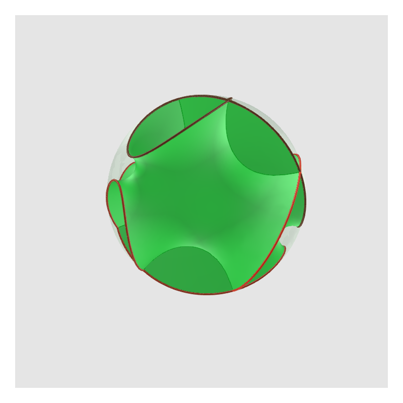
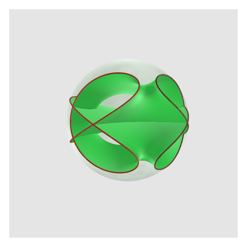
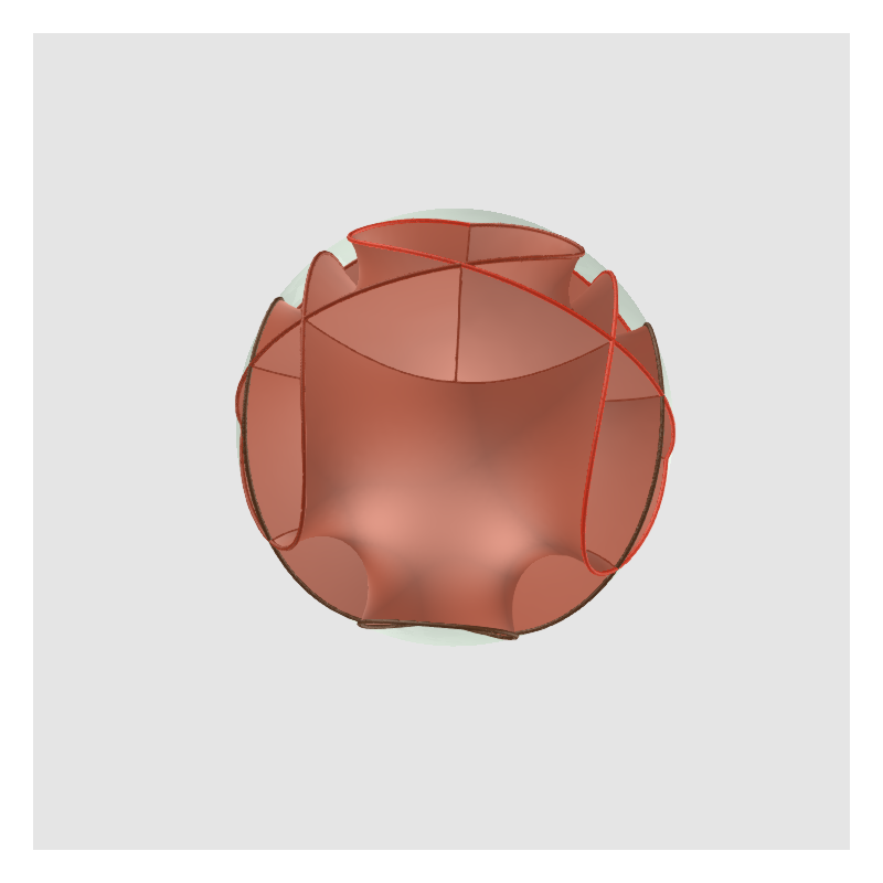
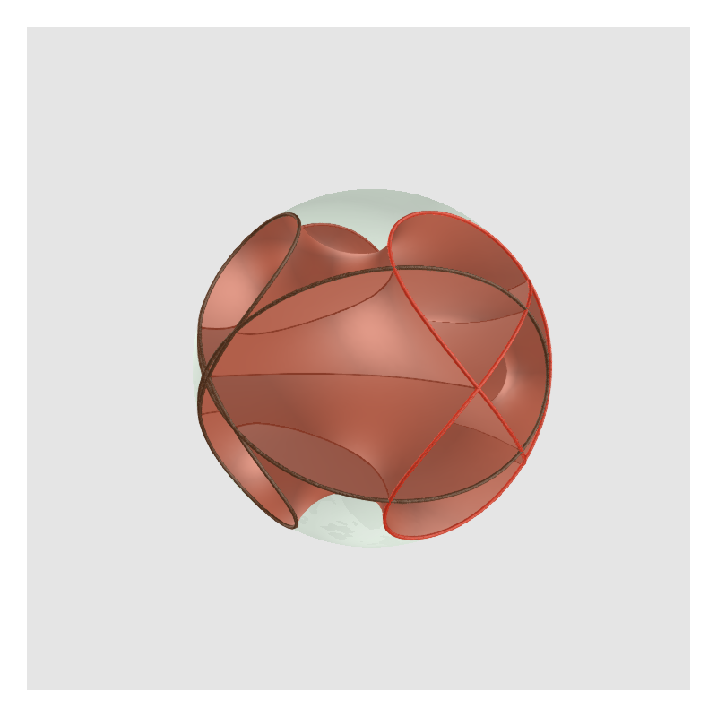
We first consider the first nontrivial eigenvalue () for varying numbers of BC, . In each case, the multiplicity of the extremal eigenvalue is three, as expected [FS15]. In Figure 7, we plot the optimal punctured disks, , for and BC. In Figures 8 and 9, we plot three linearly independent eigenfunctions associated to the first eigenvalue on their respective punctured disk for BC. For these values of , the corresponding optimal densities are plotted in Figures 10, 11, and 12. In Figures 13 and 14, we plot the corresponding (approximate) FBMS in the ball for BC. In all cases, the BC of the FBMS are positioned at very symmetric locations, as further illustrated in Figure 15. Values of and additional information about these configurations are recorded in Table 2. Additional figures, including gifs, can be found at [Oud20] and were not included here for brevity.
We now make a few more detailed remarks for the problem with the various number of BC, , considered, especially for values of that are related to the platonic solids. For some values of , we also compare to the FBMS discussed in [GL20].
For , we recover the critical catenoid, the known FBMS [FS15] that we also discussed in Section 3. Note that in Figure 7 the hole is centered within the disk and in Figure 10, the density is constant on each BC. The eigenfunctions plotted in Figure 8 exhibit symmetries and are explicitly given in Section 3; see Figure 4(right).
For , the FBMS has BC positioned with centers on an equilateral triangle inscribed on a great circle of the sphere; see Figure 13. Interestingly, the holes in the domain, , are slightly asymmetrically configured; see Figure 7. The densities plotted in Figure 10 do not exhibit symmetry. The eigenfunctions plotted in Figure 8 do not exhibit symmetries, but this could be a result of our (arbitrary) choice within the three dimensional eigenspace.
For , the FBMS has BC positioned with centers at the vertices of a regular tetrahedron; see Figure 13. This is further illustrated in Figure 15, where the BC are overlaid on a regular tetrahedron. A similar minimal surface was computed in [GL20] and the value of is within ; see Table 2. In Figure 7, the holes in the domain, , are slightly asymmetrically configured. In Figure 11, the density on the outer boundary is nearly constant and the densities on the inner boundaries are similar to each other. There is no clear structure to the eigenfunctions potted in Figure 9.
For , the FBMS has BC positioned with centers at the vertices of a triangular bipyramid; see Figure 14. In Figure 7, the holes in the domain, , are not only asymmetrically configured, but the radii of the holes vary. In Figure 11, the density on the outer boundary is nearly constant and the densities on the inner boundaries are similar to each other. Again, the eigenfunctions plotted in Figure 9 do not appear to be structured.
For , the FBMS has BC positioned with centers at the vertices of a regular octahedron; see Figure 14. This is further illustrated in Figure 15, where the BC are overlaid on a regular octahedron. Again, a similar minimal surface was computed in [GL20] and the value of is within ; see Table 2. In Figure 7, the holes in the domain, , are slightly asymmetrically configured; there is a small hole near the origin and four holes of equal radii roughly centered at the vertices of a square. In Figure 11, the density on the outer boundary is nearly constant and the densities on the inner boundaries are similar to each other.
For , the FBMS has BC positioned at the vertices of a pentagonal bipyramid. Figures of the FBMS can be found at [Oud20]. In Figure 7, the domain, , has a small (uncentered) hole surrounded by five holes.
For , the FBMS has BC positioned at the vertices of a square antiprism; see [Oud20] and Figure 15. Interestingly, we obtain for this surface, which is larger than the value obtained for the FBMS with BC at the vertices of a cube, as discussed in [GL20], with value ; see Table 2. In Figure 7, the domain, , has three smaller holes surrounded by four larger holes.
For , the FBMS has BC positioned at the vertices of a triaugmented triangular prism. Figures of the FBMS can be found at [Oud20]. In Figure 7, the domain, , has three smaller holes surrounded by five larger holes.
For , the FBMS has BC positioned at the vertices of a regular icosahedron; see Figure 14. This is further illustrated in Figure 15, where the BC are overlaid with a regular icosahedron. A similar minimal surface was computed in [GL20] and the value of is within ; see Table 2. In Figure 7, the domain, , have one small uncentered hole, surrounded by five medium-sized holes, surrounded by five larger holes.
For the FBMS is plotted in Figure 14. The FBMS has BC that are positioned with centers with triangular symmetry.
For the FBMS has irregularly located BC; a figure can be found at [Oud20]. Interestingly, we obtain for this surface, which is larger than the value obtained for the FBMS with BC at the vertices of a regular dodecahedron, as discussed in [GL20], with value ; see Table 2.
We have observed that the FBMS for and do not have BCs centered at the vertices of a platonic solid. It seems that the positions of the BCs are related to the minimizing configurations for Thompson’s problem; known as the Fekete points [Fek23, Bro20].
We note that the FBMS obtained here are closely related to the -noid surfaces; see [Web20]. It may be appropriate to the FBMS computed here as critical -noids.
5.2. Higher eigenvalues ()
Here, we consider the extremal Steklov eigenvalue problem (5), for higher eigenvalues, , . Less in known in this case and, in particular, the multiplicity of the optimal eigenvalue, and hence the dimension in which the FBMS exists, is unknown.
We recall from [FTY14] (see also Section 3) that by maximizing for odd among rotationally symmetric annuli yields an covering of the critical catenoid, a FBMS with boundary components and -th normalized Steklov eigenvalue,
We also recall the result of [FS19, Theorem 5.3], that the degenerate surface consisting of the critical catenoid glued to unit disks, is a FBMS with boundary components in dimensions with -th normalized Steklov eigenvalue,
We first consider BC and eigenvalue . In this case, the density on the outer boundary of the punctured disk becomes degenerate and resembles the discussed in Example 2.5 and displayed in Figure 3. We believe that this corresponds to the critical catenoid glued to a disc, but this is difficult to resolve using our numerical method; see Example 4.3. For other higher eigenvalues, we see similar phenomena for some initializations of . However, there are a few values of eigenvalue number and BC , that give interesting local maximizers and are very robust with respect to the initialization.
For BC and eigenvalue, we obtain a double covering of the critical catenoid as obtained by [FTY14]; see [Oud20]. The value obtained is . This is a local maximizer [FS19, Theorem 5.3]; we can obtain the value by gluing a critical catenoid to two disks.
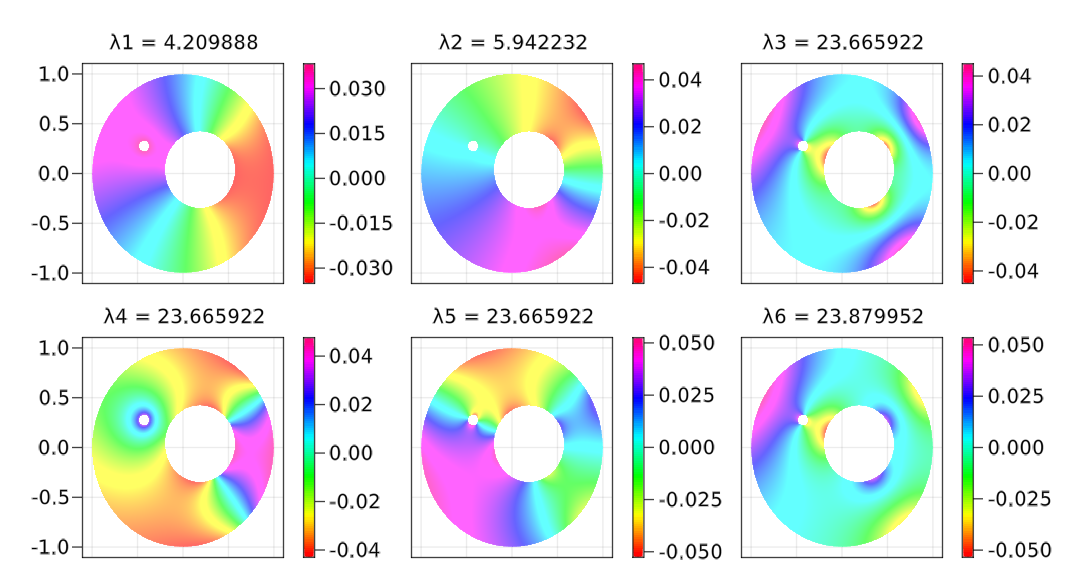
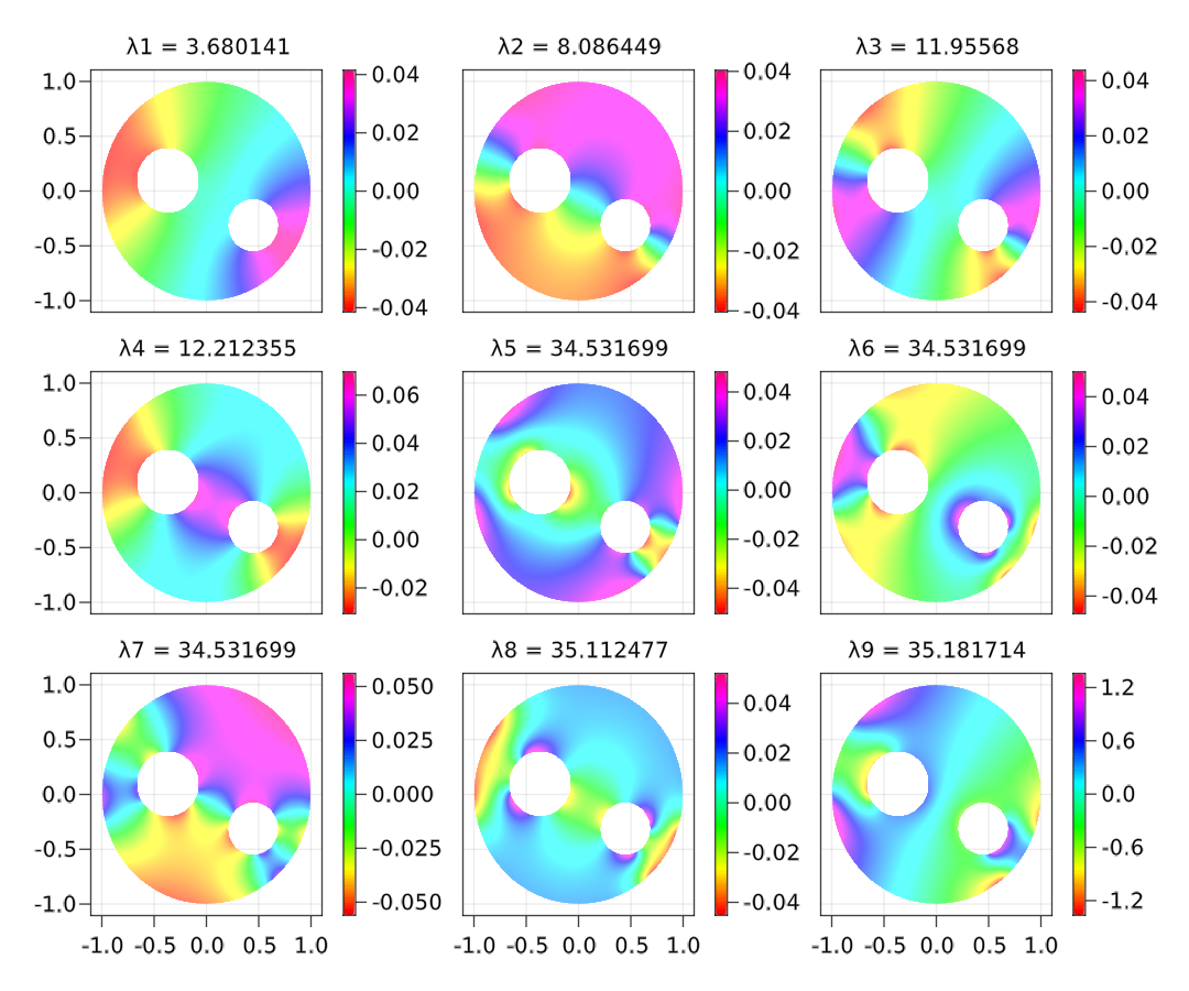
For BC the FBMS obtained by maximizing the and eigenvalues are displayed in Figure 18. If Figures 16 and 17, the first few eigenfunctions are plotted in the optimal domains, . The eigenvalues obtained are and . Note that, again, these are local maximizers since larger eigenvalues can be obtained by gluing two or four balls to the surface attained by maximizing the first eigenvalue with BC, to obtain eigenvalues and .
6. Discussion
In this paper, we developed computational methods to maximize the length-normalized -th Steklov eigenvalue, over the class of smooth Riemannian metrics, on a compact surface, , with genus and boundary components. Our numerical method involves (i) using conformal uniformization of multiply connected domains to avoid explicit parameterization for the class of metrics, (ii) accurately solving a boundary-weighted Steklov eigenvalue problem in multi-connected domains, and (iii) developing gradient-based optimization methods for this non-smooth eigenvalue optimization problem. Using the connection due to Fraser and Schoen [FS15], the solutions to this extremal Steklov eigenvalue problem for various values of boundary components are used to generate free boundary minimal surfaces.
In hindsight, it may have been better to perform these computations on a punctured sphere rather than a punctured disk, as a punctured disk distinguishes one boundary (the ‘outer’ one). In particular, by considering a punctured sphere, it may be that the holes appear more symmetrically than for a punctured disk; see Figure 7.
Beyond further exploring higher eigenvalues and higher numbers of boundary components , there are a number of interesting extensions of this work. In particular, we would be very interested to compute extremal Steklov eigenvalues on the Möbius band, torus, and other higher genus surfaces and use the associated eigenfunctions to generate free boundary minimal surfaces. We’re also interested in related extremal eigenvalue problems, involving convex combinations of Steklov eigenvalues or Steklov eigenvalues for the -Laplacian.
Acknowledgements
The authors would like to thank the Mathematics Division, National Center of Theoretical Sciences, Taipei, Taiwan for hosting a research pair program during June 15-June 30, 2019 to support this project. Chiu-Yen Kao acknowledges partial support from NSF DMS 1818948. Braxton Osting acknowledges partial support from NSF DMS 17-52202. Édouard Oudet acknowledges partial support from CoMeDiC (ANR-15-CE40-0006) and ShapO (ANR-18-CE40-0013). The authors would also like to thank Bruno Colbois, Joel Dahne, Baptiste Devyver, Alexandre Girouard, Mikhail Karpukhin, Jean Lagace and Iosif Polterovich for useful conversations.
References
- [AF12] Pedro RS Antunes and Pedro Freitas. Numerical optimization of low eigenvalues of the dirichlet and neumann laplacians. Journal of Optimization Theory and Applications, 154(1):235–257, 2012. doi:10.1007/s10957-011-9983-3.
- [AK19] Weaam Alhejaili and Chiu-Yen Kao. Maximal convex combinations of sequential steklov eigenvalues. Journal of Scientific Computing, 79(3):2006–2026, 2019. doi:10.1007/s10915-019-00925-2.
- [AKO17] Eldar Akhmetgaliyev, Chiu-Yen Kao, and Braxton Osting. Computational methods for extremal steklov problems. SIAM Journal on Control and Optimization, 55(2):1226–1240, 2017. doi:10.1137/16m1067263.
- [AO17] Pedro RS Antunes and Edouard Oudet. Numerical minimization of dirichlet laplacian eigenvalues of four-dimensional geometries. SIAM Journal on Scientific Computing, 39(3):B508–B521, 2017. doi:10.1137/16m1083773.
- [BBG17] B. Bogosel, D. Bucur, and A. Giacomini. Optimal shapes maximizing the steklov eigenvalues. SIAM Journal on Mathematical Analysis, 49(2):1645–1680, 2017. doi:10.1137/16m1075260.
- [BNW06] Richard H Byrd, Jorge Nocedal, and Richard A Waltz. Knitro: An integrated package for nonlinear optimization. In Large-scale nonlinear optimization, pages 35–59. Springer, 2006. doi:10.1007/0-387-30065-1_4.
- [BO16] Beniamin Bogosel and Edouard Oudet. Qualitative and numerical analysis of a spectral problem with perimeter constraint. SIAM Journal on Control and Optimization, 54(1):317–340, 2016. doi:10.1137/140999530.
- [Bro20] Kevin Brown. Min-energy configurations of electrons on a sphere. http://mathpages.com/home/kmath005/kmath005.htm, 2020.
- [Dit04] Bodo Dittmar. Sums of reciprocal Stekloff eigenvalues. Mathematische Nachrichten, 268(1):44–49, 2004. doi:10.1002/mana.200310158.
- [DKL14] Marc Dambrine, Djalil Kateb, and Jimmy Lamboley. An extremal eigenvalue problem for the Wentzell–Laplace operator. In Annales de l’Institut Henri Poincare (C) Non Linear Analysis, 2014. doi:10.1016/j.anihpc.2014.11.002.
- [ESI+07] Ahmad El Soufi, Saïd Ilias, et al. Domain deformations and eigenvalues of the dirichlet laplacian in a riemannian manifold. Illinois Journal of Mathematics, 51(2):645–666, 2007. doi:10.1215/ijm/1258138436.
- [Fek23] Michael Fekete. über die verteilung der wurzeln bei gewissen algebraischen gleichungen mit ganzzahligen koeffizienten. Mathematische Zeitschrift, 17(1):228–249, 1923. doi:10.1007/bf01504345.
- [FS11] Ailana Fraser and Richard Schoen. The first steklov eigenvalue, conformal geometry, and minimal surfaces. Advances in Mathematics, 226(5):4011–4030, 2011. doi:10.1016/j.aim.2010.11.007.
- [FS13] Ailana Fraser and Richard Schoen. Minimal surfaces and eigenvalue problems. Contemporary Mathematics, pages 105–121, 2013. doi:10.1090/conm/599/11927.
- [FS15] Ailana Fraser and Richard Schoen. Sharp eigenvalue bounds and minimal surfaces in the ball. Inventiones mathematicae, 203(3):823–890, 2015. doi:10.1007/s00222-015-0604-x.
- [FS19] Ailana Fraser and Richard Schoen. Some results on higher eigenvalue optimization. preprint, arXiv:1910.03547, 2019.
- [FTY14] Xu-Qian Fan, Luen-Fai Tam, and Chengjie Yu. Extremal problems for steklov eigenvalues on annuli. Calculus of Variations and Partial Differential Equations, 54(1):1043–1059, 2014. doi:10.1007/s00526-014-0816-8.
- [GL99] Frederick Gardiner and Nikola Lakic. Quasiconformal Teichmüller Theory. American Mathematical Society, 1999. doi:10.1090/surv/076.
- [GL20] Alexandre Girouard and Jean Lagacé. Large steklov eigenvalues via homogenisation on manifolds. preprint, arXiv:2004.04044, 2020.
- [GLS16] Alexandre Girouard, Richard S Laugesen, and BA Siudeja. Steklov eigenvalues and quasiconformal maps of simply connected planar domains. Archive for Rational Mechanics and Analysis, 219(2):903–936, 2016. doi:10.1007/s00205-015-0912-8.
- [GP12] Alexandre Girouard and Iosif Polterovich. Upper bounds for steklov eigenvalues on surfaces. Electronic Research Announcements in Mathematical Sciences, 19(0):77–85, 2012. doi:10.3934/era.2012.19.77.
- [GP17] Alexandre Girouard and Iosif Polterovich. Spectral geometry of the steklov problem. Journal of Spectral Theory, 7(2):321–359, 2017. doi:10.4171/jst/164.
- [Hen86] Peter Henrici. Applied and Computational Complex Analysis. John Wiley & Sons, 1986.
- [JGHW18] Miao Jin, Xianfeng Gu, Ying He, and Yalin Wang. Conformal Geometry. Springer International Publishing, 2018. doi:10.1007/978-3-319-75332-4.
- [Kar17] Mikhail Karpukhin. Bounds between laplace and steklov eigenvalues on nonnegatively curved manifolds. Electronic Research Announcements in Mathematical Sciences, 24:100–109, 2017. doi:10.3934/era.2017.24.011.
- [KLO17] Chiu-Yen Kao, Rongjie Lai, and Braxton Osting. Maximization of laplace-beltrami eigenvalues on closed riemannian surfaces. ESAIM: Control, Optimisation and Calculus of Variations, 23(2):685–720, 2017. doi:10.1051/cocv/2016008.
- [Li19] Martin Li. Free boundary minimal surfaces in the unit ball: recent advances and open questions. preprint, arXiv:1907.05053, 2019.
- [LP15] Pier Domenico Lamberti and Luigi Provenzano. Viewing the steklov eigenvalues of the laplace operator as critical neumann eigenvalues. In Trends in Mathematics, pages 171–178. Springer International Publishing, 2015. doi:10.1007/978-3-319-12577-0_21.
- [Mar14] Étienne Martel. Le spectre de steklov de la boule trou’ee. Journal du coloque des étudiants de 1er cycle en mathématiques de l’Université Laval, 2014.
- [MP20] Henrik Matthiesen and Romain Petrides. Free boundary minimal surfaces of any topological type in euclidean balls via shape optimization. preprint, arXiv:2005.06051, 2020.
- [OK13] Braxton Osting and Chiu-Yen Kao. Minimal convex combinations of sequential laplace–dirichlet eigenvalues. SIAM Journal on Scientific Computing, 35(3):B731–B750, 2013. doi:10.1137/120881865.
- [OK14] Braxton Osting and Chiu-Yen Kao. Minimal convex combinations of three sequential laplace-dirichlet eigenvalues. Applied Mathematics & Optimization, 69(1):123–139, 2014. doi:10.1007/s00245-013-9219-z.
- [Olv17] Peter J Olver. Complex analysis and conformal mapping. University of Minnesota, 2017.
- [Ost10] Braxton Osting. Optimization of spectral functions of dirichlet–laplacian eigenvalues. Journal of Computational Physics, 229(22):8578–8590, 2010. doi:10.1016/j.jcp.2010.07.040.
- [Oud04] Édouard Oudet. Numerical minimization of eigenmodes of a membrane with respect to the domain. ESAIM: Control, Optimisation and Calculus of Variations, 10(3):315–330, 2004. doi:10.1051/cocv:2004011.
- [Oud20] É. Oudet. personal website. https://www-ljk.imag.fr/membres/Edouard.Oudet/research/SteklovMin/index_n.php, 2020.
- [Tre18] Lloyd N. Trefethen. Series solution of laplace problems. The ANZIAM Journal, 60(1):1–26, 2018. doi:10.1017/s1446181118000093.
- [Web20] Matthias Weber. Bloomington’s virtual minimal surface museum. https://minimal.sitehost.iu.edu/archive/Spheres/Noids/Jorge-Meeks/web/index.html, 2020.
- [Wei54] Robert Weinstock. Inequalities for a classical eigenvalue problem. Indiana University Mathematics Journal, 3(6):745–753, 1954. doi:10.1512/iumj.1954.3.53036.
- [ZYZ+09] Wei Zeng, Xiaotian Yin, Min Zhang, Feng Luo, and Xianfeng Gu. Generalized koebe’s method for conformal mapping multiply connected domains. In 2009 SIAM/ACM Joint Conference on Geometric and Physical Modeling, pages 89–100, 2009. doi:10.1145/1629255.1629267.