Mapping the inhomogeneous Universe with Standard Sirens: Degeneracy between inhomogeneity and modified gravity theories2020Mapping the inhomogeneous Universe with Standard Sirens: Degeneracy between inhomogeneity and modified gravity theories–23
![[Uncaptioned image]](2007.15020v2/ORCIDiD_icon.png)
Abstract
The detection of gravitational waves (GWs) and an accompanying electromagnetic (E/M) counterpart have been suggested as a future probe for cosmology and theories of gravity. In this paper, we present calculations of the luminosity distance of sources taking into account inhomogeneities in the matter distribution that are predicted in numerical simulations of structure formation. In addition, we show that inhomogeneities resulting from clustering of matter can mimic certain classes of modified gravity theories, or other effects that dampen GW amplitudes, and deviations larger than to the extra friction term , from zero, would be necessary to distinguish them. For these, we assume mock GWs sources, with known redshift, based on binary population synthesis models, between redshifts and . We show that future GW detectors, like Einstein Telescope or Cosmic Explorer, will be needed for strong constraints on the inhomogeneity parameters and breaking the degeneracy between modified gravity effects and matter anisotropies by measuring at and level with and events respectively.
Keywords:
methods: theory – cosmology: gravitational waves - inhomogeneous universe - modified gravity1 Introduction
The standard model of cosmology Lambda-Cold-Dark-Matter (CDM) is based on the assumption that the universe is homogeneous and isotropic, which is supported on large-scales by precise CMB measurements (Akrami & et al 2020). These symmetry hypotheses lead to the well-known Friedmann-Lemaître-Robertson-Walker (FLRW) metric to describe the Universe’s geometry. Although the standard model has passed successfully many tests, various “tensions” exist (Verde et al. 2019), so independent confirmations of its basic assumptions are important.
Tests checking the homogeneity and isotropy of the Universe, based on electromagnetic (E/M) observations, have been proposed and performed in the literature (for example Clifton et al. 2008; Busti et al. 2012a; Dhawan et al. 2018), showing consistency of the standard model, but require more data (so far simple inhomogeneous models are consistent with homogeneity at level). At the same time, the robustness of some basic CDM assumptions, like the isotropy or the spatial curvature of the Universe, have recently been under debate (see Nielsen et al. 2016; Rubin & Hayden 2016; Colin et al. 2019; Rubin & Heitlauf 2020; Handley 2019; Di Valentino et al. 2020; Efstathiou & Gratton 2020; Heinesen & Buchert 2020; Migkas et al. 2020). Most of the above analyses require good, model-independent distance measurements, which in general, are difficult to obtain.
The first direct detection of GWs with an E/M counterpart (‘‘standard siren’’11 1 Historically, “Standard Sirens” refer to every compact binary - BBH, BNS, BH-NS - with or without an E/M counterpart (Schutz 1986; Holz & Hughes 2005). Here we are going to use the term as equivalent to any GW detection that has also independent redshift information.) (Abbott et al. 2017d) presents an alternative way to study fundamental physics and provide an independent probe for assessing our basic assumptions for the Universe. The simultaneous determination of the luminosity distance, based solely on general relativity (GR), and the localisation of the source from the E/M observation, which was demonstrated for example with the first observation of a binary neutron star (Abbott et al. 2017b), has opened new possibilities to test our cosmological theories, in a model-independent way, by exploiting the observed distances.
There are already various proposals of how the luminosity distances inferred from GWs standard sirens observations can be used for cosmology. Examples include the determination of the Hubble parameter (Schutz 1986; Abbott et al. 2017c), constraints on the cosmological parameters (Cutler & Holz 2009a), the distance duality relation (Hogg et al. 2020) and measurement of peculiar velocities in the local universe to probe gravity and structure growth (Palmese & Kim 2020). Moreover, (Seto et al. 2001) and (Yagi et al. 2012) suggest a direct measurement of cosmic acceleration with GW sirens by observing a phase shift in the signal (a deviation from the value that is expected in an FLRW spacetime, can be a sign for deviations from the Cosmological Principle’s homogeneity). Further applications of standard sirens include constraints on cosmic anisotropies, e.g. the dipole anisotropy (Cai et al. 2018; Lin et al. 2018), and the spatial curvature, e.g. (Wei 2018).
At the same time, various classes of modified theories of gravity predict that distances inferred from GWs deviate from those of their E/M counterpart. These theories include a number of new degrees of freedom to dynamically describe the late-time acceleration of the Universe (Joyce et al. 2016; Ferreira 2019, e.g.). The additions to GR can introduce several new effects on the propagation of GWs, like a different propagation speed or an amplitude decay, compared to photons (Saltas et al. 2014; Saltas et al. 2018; Nishizawa 2018; Amendola et al. 2018; María Ezquiaga & Zumalacárregui 2018). However, so far tests with current GWs observations (Abbott et al. 2016; Abbott et al. 2019b; Abbott et al. 2019a), that investigate a massive graviton and phenomenological models of extra-dimensions, show consistency with GR.
As laid out above, several different physical processes can lead to a reduction in the amplitude of GWs as they propagate through the Universe. In this paper, we investigate the measurement of luminosity distances of GWs propagating through inhomogeneities and under the effects of modified gravity theories. To model the effects of inhomogeneities, different approaches have been taken in the literature (see e.g. Fleury 2015; Helbig 2020, for an overview). Perturbations around FLRW (Bertacca et al. 2018) show negligible effects for the near future detectors. Here we will concentrate on modelling inhomogeneities with the Dyer-Roeder (DR) relation (Dyer & Roeder 1972) and a modification of it, the modified DR relation (mDR) (Clarkson et al. 2012), which approximate better small-scale inhomogeneities. In a previous study (Yoo et al. 2007) investigated the impact of inhomogeneities on GWs, concentrating only on an extreme inhomogeneous (empty) DR universe, with a uniform distribution of same mass objects. The focus of that study was, however, on the information that could be obtained about the lenses, using strong lensing of GW events. Moreover, previous studies (Cutler & Holz 2009a; Camera & Nishizawa 2013; Congedo & Taylor 2019) investigated the impact of inhomogeneities in a statistical sense, deriving constraints on the cosmological parameters from joint weak lensing and gravitational waves observations, showing a potential for accuracy. At the same time, an improved modelling of the lensing magnification distribution, assuming a non-Gaussian PDF (Hirata et al. 2010; Shang & Haiman 2011) or the extreme case of empty beams (Linder 2008), can lead to further enhancement in accuracy. The possibility for cosmological constraints from the anisotropy of GWs observations only (without a counterpart) was also studied in (Namikawa et al. 2016). In this paper we investigate the possible constraints from future GWs observations, on arbitrary inhomogeneous models and on inhomogeneous models derived from cosmological N-body simulations. We also examine possible degeneracies of these effects with modified gravity theories and how these could be broken with next generation GW detectors, more specifically Einstein Telescope (ET) and Cosmic Explorer (CE) (Maggiore et al. 2020; Abbott et al. 2017a).
The paper is structured as follows: In Section 2 we study the effects on the GW luminosity distance produced by modified gravity theories and an inhomogeneous background and present the various models we are interested in constraining, in Section 3 we describe the cosmological simulations and the numerical techniques employed, in Section 4 we discuss our results and in Section 5 we summarise our findings and discuss possible future directions.
2 Distances from GWs
A GW detection with an E/M counterpart leads to two observable quantities for cosmology: the luminosity distance to the source22 2 There is a degeneracy with orbit inclination which can be lifted with precise observations of the two polarisations or E/M observations (Baker et al. 2019). and its redshift . The dominant, quadrupole contribution (Maggiore 2008) gives:
| (1) |
where is the amplitude of the GW, is the speed of light, Newton’s constant, the frequency of the GW at the observer and is the “redshifted chirp mass” and is the chirp mass, with and the individual masses of the compact objects. For binary black hole systems, the information of redshift is completely degenerate with the chirp mass, and thus a cosmological model, which makes a correspondence between and , cannot be constrained by a GW observation alone33 3 For binary neutron stars, the tidal effects can permit a direct redshift measurement.. Redshift is inferred by an E/M counterpart, or by a galaxy that is identified as the host of a GW event (Nishizawa 2017). Hereafter, we consider GW events where the redshift is known. Hence, we consider the case where we have two independent observables, the redshift to the source obtained by E/M observations and its luminosity distance, inferred by the GW detection.
In general, the redshift and luminosity distance have been measured by a number of E/M observations. The measured luminosity distance, is consistent with that of a flat CDM universe (ignoring radiation):
| (2) |
where are the dimensionless densities for matter and the cosmological constant respectively and the Hubble parameter. This fact allows us to assume that the luminosity distance is unique with the underlying cosmological model, i.e., (z). However, this assumption should be carefully inspected with GW observations.
Any deviations between the luminosity distance derived from the GW and the one calculated from the standard CDM formula, given the redshift of the E/M counterpart, are potential signs of differences caused by systematic deviations from the underlying model assumptions. In the following sections we review the effects caused by modified gravity theories and inhomogeneities in the Universe, and the possibility to constrain them.
2.1 Modified Gravity
We start by reviewing the effects of modified gravity that can lead to a decrease on the observed amplitude of a GW44 4 We note that modified gravity models can also impact the background expansion and hence affect photon propagation (Belgacem et al. 2018b; María Ezquiaga & Zumalacárregui 2018), but we are going to neglect this here.. We are interested in these, due to their possible degeneracy with the presence of inhomogeneities, that also result in a drop of the observed amplitude (Section 2.2). The new additions to GR can introduce several new effects on the propagation of GWs (Saltas et al. 2014; Saltas et al. 2018; Nishizawa 2018; Amendola et al. 2018; María Ezquiaga & Zumalacárregui 2018). These are model dependent, but effectively they are summarised in the equation below (primes denote derivatives w.r.t. conformal time):
| (3) |
where the standard evolution of tensor perturbations is modified by an additional friction term, the GW propagation speed, the graviton mass and a source term. The case where are equal to zero and = 1 corresponds to standard GR. Focusing only on the terms affecting the amplitude, and neglecting any source terms, we have:
| (4) |
The general class of theories that predict a friction term is the class of scalar-tensor theories (Saltas et al. 2018) and theories that break some fundamental assumptions, introducing for example extra-dimensions (Corman et al. 2020) or theories where non-local terms appear at the level of the quantum effective action (Belgacem et al. 2018a). Here, because of the friction term in front of the Hubble drag, the distances measured from GWs and E/M signals can differ. Usually the GWs distance is compared to the standard CDM one - see eq. (2) - which is calculated using the redshift obtained from the E/M observation. Then, the relation between the GW and E/M luminosity distance is given by (Belgacem et al. 2018a; Belgacem et al. 2020):
| (5) |
For constant , it is easy to solve this relation analytically:
| (6) |
This case was investigated in (Nishizawa & Arai 2019), where the authors found that future constraints on can reach . Similarly, strong observational bounds on scalar-tensor theories have been predicted in (D’Agostino & Nunes 2019). The GW170817 event provided a very loose constraint on , in the range , when considered a constant. The constraints are weaker when is Taylor-expanded as , with the look-back time, and are fitted (Arai & Nishizawa 2018). Throughout this paper, we assume that is constant.
2.2 Inhomogeneous models
Inhomogeneous models affect both GWs and E/M distances on the same way. This is because they assume that both signals travel in paths that deviate from the smooth background, although without altering GR. A critical investigation of these effects is necessary, since comparing the GWs distance with the one based on CDM can lead to the false assumption of a deviation from the standard model that can be attributed to a modified GW propagation, while the source of the discrepancy would be a simplified approximation of the E/M distance, when inhomogeneities should be taken into account.
Below we review how different models can affect the angular diameter distance, and hence the luminosity distance that we would infer.
2.2.1 The FLRW distance
As a reference, we recall that for a smooth, homogeneous universe, the angular diameter distance , is given from the differential equation (Clarkson et al. 2012):
| (7) |
where .
2.2.2 The DR distance
The Dyer-Roeder (DR) distance models a bundle of rays travelling through voids (“empty beams”), while assuming that the general background follows the standard FLRW geometry. Its usefulness is due to the fact that it yields the largest possible distance (for a given redshift) for light bundles which have not passed through a caustic (Schneider et al. 1992).
On the other hand, if the universe is not very clumpy, the Dyer-Roeder distances and those of the smooth FLRW universe are not too different (Fukugita et al. 1992; Schneider et al. 1992).
The DR distance is given by the solution to the following differential equation:
| (8) |
where and only an extra factor - the inhomogeneity factor - has been added to the RHS compared to the FLRW case. For , we return to the standard FLRW result, while describes an “empty” beam, with the intermediate values denoting different levels of under-dense regions. Values of correspond to over-densities.

2.2.3 The modified DR distance
As we mentioned above, the DR approximation assumes that we can disentangle the inhomogeneities encountered by photons from the background density, which assumes a smooth FLRW background. However, photons only experience the local curvature and expansion, so a simple modification would be to take into account the different expansion dynamics caused by the local anisotropies. This leads to a modified version of the DR formula55 5 Please note, that the original equation in (Clarkson et al. 2012, eq. (82)) includes typos and that we show here the correct equation, including and a missing factor of two.:
| (9) |
with , where the inhomogeneous parameter , has now been included in all the density terms (), but its derivatives have been neglected, as in (Clarkson et al. 2012).
As can be seen from Figure 1, the distance of the DR and mDR approximations (in the extreme case of totally empty beams, i.e. ) vs the FLRW case can become quite important for high-z observations, and a careful modelling is needed if we want to extract accurate parameters.
Although these redshifts () are large enough to reach homogeneity, in most cases we observe focused light “beams”, so we usually do not see an average over the whole sky (Weinberg 1976). Hence, inhomogeneities at relatively large redshifts still need to be accounted for (Fleury et al. 2017; Dhawan et al. 2018).
2.2.4 The inhomogeneity parameter
The distances above are not mathematically exact solutions of GR, but are effective models trying to capture the impact of inhomogeneities on observed distances (Schneider et al. 1992; Mattsson 2010). Different parameterisations have been suggested in the literature for such effective models. Here we will focus on the following two (Linder 1988; Bolejko 2011):
- 1.
.
- 2.
,
where are arbitrary constants, the function is chosen as to be consistent with the weak lensing approximation66 6 This was investigated only for the DR model in (Bolejko 2011). (Bonvin et al. 2006) and denotes the average present-time density contrast along a ray, with . The two parameterisations are connected at small redshifts via and (see Appendix B for details). We obtain the values of from cosmological simulations described in the next section.

2.3 Constraining the inhomogeneity parameter
The differential equations above give the angular diameter distance in each specific case. We solve them, using as initial conditions and , and assuming, for consistency with the later sections, the cosmological parameters of WMAP9 (Hinshaw et al. 2013), with ().
The choice of priors on the standard cosmological parameters, based on the concordance cosmological model, let us proceed to constrain the “clumpiness” of the universe alone, or else the fraction of DM in compact objects. This has been attempted before, in a somewhat more simplified way (with constant ), for Supernovae (SN) and Gamma-ray Bursts (GRBs) in (Bretón & Montiel 2013; Helbig 2015a; Helbig 2015b), however our work extends the analysis to higher redshifts, uses the full non-linear clustering found in cosmological N-body simulations and introduces different systematics, related to the GW observations77 7 Previous studies (Busti et al. 2012b; Fleury et al. 2013; Dhawan et al. 2018) that have fitted simultaneously the cosmological parameters and do not find a significant change of the standard values of and - see also Appendix D..
To transform to luminosity distances we use the reciprocity distance relation (Etherington 1933; Ellis 2007), which holds for an arbitrary spacetime geometry, as long as photons are conserved, and connects luminosity and angular diameter distances via:
| (10) |
Concerning the errors in distance determination, we follow the analysis of (Cai & Yang 2017). We neglect the errors of the spectroscopic redshift determination, since they are negligible compared to the errors in the luminosity distance. For the errors in the GW luminosity distance we take into account the uncertainty from instrumental errors (Li 2015):
| (11) |
where the Signal-to-Noise Ratio (SNR) , depends on the chirp mass of the source, its redshift and the detector’s sensitivity, and the factor of comes from marginalising over the uncertainty of the inclination’s determination. Also, there is an additional error, connected to weak lensing effects88 8 This formula is extrapolated from SN observations (Jönsson et al. 2010). Theoretical models, based on numerical simulations (Holz & Linder 2005; Marra et al. 2013; Fleury et al. 2015), each one using different techniques (including inhomogeneous models) are consistent with each other, and the one used above, within observational errors. (Sathyaprakash et al. 2010; Zhao et al. 2011):
| (12) |
Finally, the total error (for a single event) is:
| (13) |
We add these errors in quadrature, assuming they originate from independent sources, as one part is systematic and the other statistical. In the following, when calculating the fit, in order to estimate the errors we are going to consider the luminosity distance of the “true” case as their source. We assume that all sources are independent, and include a scatter in their distances, allowing them to follow a normal distribution , with the mean and the standard deviation, for each redshift, as shown in Figure 2. We describe in more detail the calculation of in the next subsection.
2.4 SNR calculation
We estimate the SNR as:
| (14) |
where is the Fourier transform (FT) of the amplitude of the GW, is the characteristic noise curve of each detector (see Appendix E) and is two times the frequency at the innermost stable circular orbit, where the analytical methods fail.
For the FT of the amplitude of a binary system we follow (Buonanno 2007; Maggiore 2008) and calculate the sky-averaged value, over all possible directions and inclinations. Since we are only interested in the amplitude’s norm, the relevant phase factors are simplified. Then, for an L-shaped detector, like LIGO or CE, we have:
| (15) |
For a V-shaped detector, like ET, with an opening angle of degrees and three arms (Regimbau et al. 2012), we find only a difference in the normalisation coefficient due to the different detector configuration. This leads to the factor being substituted by in above equation.
2.5 Merger Rates
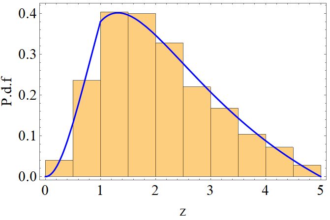
The redshift distribution of potentially observable GW sources (Figure 3) is given by (Zhao et al. 2011):
| (16) |
where is the comoving distance and R(z) the merger rate (number of events per year) of compact binary systems with E/M counterparts (BH-NS NS-NS) given by (Schneider et al. 2001; Cutler & Holz 2009b; Zhao et al. 2011):
| (17) |
The rates are based on the binary population synthesis code SeBa (Portegies
Zwart & Yungelson 1998), where the main assumptions used for the calculation in (Schneider et al. 2001) are: (i) the mass
of the primary star is determined using the mass function described by (Scalo 1986) between and , (ii) For a given , the mass of the secondary star is randomly selected from a uniform distribution between a minimum of and the mass of the primary star, (iii) The semi-major axis distribution is taken flat in ranging from Roche-lobe contact up to and (iv) The initial eccentricity distribution is independent of the other orbital parameters. The results are constrained by our Galaxy, but, using the observed star formation rate, they are extended until redshift .
In the rate equation - eq. (16) - we can assume, without affecting our results, the estimates for a smooth FLRW cosmology, since we are interested in the deviations of distances between some observed sources. This should not be affected by how we populate the sources (see also Appendix A). The evolution of merger rate as a function of redshift has also been constrained from the up-to-date detections (Abbott et al. 2019c), but with poor results so far due to the small statistics. Only the presence of a significant number of lensed events could change considerably the distribution, however this does not seem to be the case (Hannuksela et al. 2019). Nevertheless, the method proposed in this paper is not invalidated by the distribution of sources, however the latter is important for the estimated error contours.

3 Simulations
To calculate realistic density anisotropies, we rely on cosmological dark matter only simulations run with Gadget-4 (Springel et al. 2020) for the LEGACY project.
The latter is composed by two primary volumes of Mpc/h and Mpc/h box sizes run down to with resolution elements, as well as a set of zoom-in simulations on the larger box, with size Mpc/h, and an effective resolution of . These simulations have been designed to sample , and of the mean density value as well as extremely high (cluster) and very low (void) density regions and are therefore ideal to study different environmental effects.
For our analysis, we use the data from the big Mpc/h run, at , with an effective resolution of particles and mass resolution which will suffice for the purpose of this investigation.


3.1 Cloud-in-cells implementation
For our simulation box, we perform a Cloud-in-Cell (CiC) interpolation scheme to deposit the particles to specific grid points (Hockney & Eastwood 1988). The weighting function is:
| (18) |
where is the resolution of the CiC box and the centres of the grid cells.
3.1.1 Density calculation
We investigate a number of resolutions, from a grid with cells to a grid with cells. From these we calculate the density anisotropies along straight trajectories and calculate the mean value for each ray99 9 See Appendix C for details. to find (Figure 4). For all resolutions the mean 3D density contrast is zero.
As expected, the lowest resolution () returns a distribution closer to the mean contrast, since we average out on larger volumes. The highest resolution run () produces a distribution with tails that describe the under/over-densities at small scales. In the following we exploit the data from this run.
4 Results
4.1 Inhomogeneity Constraints
To fit our model with GW standard sirens observations we use a goodness of fit defined as:
| (19) |
where the summation includes all distinct observations. We use here mock GWs events, unless stated otherwise. This corresponds to a conservative limit for future detectors (Abbott et al. 2017a; Maggiore et al. 2020) for redshifts per year cycle, but seems to be a quite optimistic limit for a -year LISA mission (Klein et al. 2016) and the next observing run of the current GWs detectors (Abbott et al. 2018). For this reason, we are going to use the sensitivity curve of Einstein Telescope (ET) (Maggiore et al. 2020) - the most conservative between the future generation GW detectors, as our standard reference when investigating future constraints. Current detectors will not be able to put any useful constraints. We return to this at the end of the next subsection. denotes the distance based on the inhomogeneous or modified gravity models we study. For each “fitted” distance, the parameters take all the values between to when constraining an inhomogeneous model and varies between to for the modified gravity parameterisation, based on a standard grid sampling method, with resolution chosen for convergence, and where for each point a different value for is calculated. The redshift of the sources are randomly drawn from the distribution in Figure 3, where the maximum possible redshift is chosen as . We denote as the “true” distance, that would be specified in each case (see below), and with this we calculate the errors using eq. (13).
More specifically, the steps we take are the following:
- 1.
We choose the number of sources we want to use, .
- 2.
We choose the maximum redshift of the sources, .
- 3.
We generate an array of redshifts of length and maximum value . If we use the densities calculated from the simulation, we similarly generate an array of s, randomly drawn from the high-resolution distribution of Figure 4.
- 4.
We select our “true” distance from either the DR, mDR, FLRW or modified gravity model and we transform the redshifts generated above to a list of distances.
- 5.
We finally calculate the constraints that can be put on the inhomogeneity/modified gravity parameters, by fitting with a theoretical model ( above).
In our contour fits we plot the confidence intervals. The filled ones correspond to the DR model and the dashed ones to the mDR model.

4.1.1 Scaling with sources and redshift
We begin by investigating how the constraints scale with number of sources and with maximum value of redshift. For this we simulate and sources and investigate readshifts . The filled contours correspond to contraints based on the DR distance and the dashed ones on the mDR distance, both using the first parameterisation of section 2.2.4 ().
Our results are summarised in Figure 5. We start by testing how well we recover an inhomogenous DR model with input parameters and a FLRW model. First of all, in both cases we recover the input models at the level and in the latter case the model is constrained significantly.
Secondly, we observe a similar trend as (Clarkson et al. 2012), in that different inhomogeneous models can lead to quite distinct results as shown by the dashed-line contours compared to the solid line ones. These uncertainties in the modelling, limit precision cosmology in terms of being able to constrain physical properties (e.g. the optical depth), modified gravity theories or parameterisations of the dark energy equation of state to high accuracy (Chevallier & Polarski 2001; Linder 2003).
Thirdly, as expected, we observe that both parameterisations lead to more stringent constraints when more events are detected. Also, high-z observations are required to better distinguish between the models, being consistent with Figure 1. The two parameters are almost unconstrained in the DR case, while can reach accuracy if a mDR model is considered. However, the latter seems almost unaffected by either or the number of sources.
A similar conclusion results from the analysis of GW sources, but for different maximum redshifts . The relevant figures demonstrate clearly that the maximum redshift is a much more important parameter than the number of sources, since the different distance measures start to deviate significantly at larger redshifts. This is true even if the underlying population synthesis model leads to quite similar distribution of SNR per maximum redshift - see Appendix E. This would allow a direct probe of the scales where the Universe reaches homogeneity, especially if the errors can be reduced by de-lensing techniques (Lewis & Challinor 2006).
We should note here that we repeated a similar procedure with current detectors (aLIGO). From the sources that were observed by ET, only passed the trigger limit of . As a result, in all cases current detectors leave the whole parameter space unconstrained. This emphasises the need for new ground-based detectors for cosmological studies.
4.1.2 Constraints from numerical simulations
We now follow the same procedure exploiting the second parameterisation in 2.2.4. This has a clearer physical interpretation, related directly with the density anisotropies along the line-of-sight. Here we keep the maximum redshift and the number of sources fixed at , and consider as “fiducial” distances the ones based on the parameterisation ().
To calculate them, we follow the following procedure: For each mock source, we pick randomly a 1D density contrast from the high resolution distribution of Figure 4 and a random redshift as before. We calculate the “true” distance by numerically solving the DR equation, since in this model this would be equivalent to the weak lensing approximation. With them, we try to constrain the DR and mDR models, based on the first parameterisation of section 2.2.4 ().


An example of the possible deviation is shown in Figure 6, where we have used the two limiting cases () based on our simulations. Since these correspond to small perturbations in the metric, the effects are small. More extreme cases are shown in Figure 7. The constraints on are shown in Figure 8. We see that the presence of small inhomogeneities along the ray results in distance estimates consistent with FLRW, confirming some previous semi-analytical and numerical studies (Mörtsell 2002; Kaiser & Peacock 2016; Adamek et al. 2019). However, we note that the result only holds for weak inhomogeneities1010 10 Note that the maximum mean under-density we find in our simulations is of the order of ., since non-linear effects could potentially have an important contribution (Bolejko 2018, e.g.).
4.2 Modified gravity effects
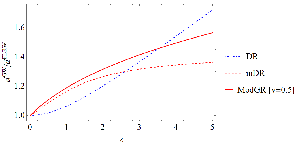


As we have seen, the measurement of accurate distances from GWs can be in itself an independent probe of the inhomogeneity of our Universe. Inhomogeneous models with under-densities, in general predict larger distances than the FLRW ones and this effect could have more general implications, since every physical mechanism that modifies the amplitude of the wave, could lead to a similar deviation (María Ezquiaga & Zumalacárregui 2018; Belgacem et al. 2018a; Belgacem et al. 2019; Wei 2019; Zhou et al. 2019). Figure 9 provides a simple example of this correspondence.
Of course, an inhomogeneous universe will lead to a different propagation than FLRW, for both photons and GWs, however this strengthens our point that an accurate determination of the underlying geometry is necessary before investigating deviations of modified gravity models, which are usually compared with the expectation from FLRW. This could lead to important implications if the underlying geometry is not FLRW, since in this case modified gravity effects are degenerate with respect to inhomogeneous models.
However, as can been seen in the example of Figures 9, precise distance measurements, that would significantly reduce the observed errors, could disentangle the two effects in simple models, since they have a different redshift dependence (concave vs convex curves). Also it is worth noticing that inhomogeneous models could possibly only mimic gravity modifications that lead to increased distance, so with . Hence, although the degeneracy between inhomogeneities and modified gravity models concern mainly small, positive values of , that will be investigated in more detail below, since the sign of and even its redshift dependence are not presently constrained significantly, we cannot a priori break this degeneracy.
For a more detailed comparison, we repeat our fit, where in this case we use as “true” input a modified gravity model with effective parameter . We then constrain the values of for the two inhomogeneous models, using mock observations that reach . This leads to Figure 10. We see that even a small number of sources () results in quite strong constraints, indicating that only extreme inhomogeneities can lead to equivalent results. Of course, this is an arbitrary example, but it demonstrates our previous point that “realistic” inhomogeneous models are not able to mimic all values of the modification parameters. The best fit parameters lead to distances as shown in Figure 9, which deviate significantly from the FLRW ones and are probably unphysical. However, modified gravity models that result in less extreme values of would not be distinguishable from inhomogeneous models given present observational facilities.
Finally, we invert the procedure and exploiting the parameterisation we try to fit the best modified gravity model and put limits to the values of that could be disentangled from small inhomogeneity effects. We demonstrate this effect and quantify the number of events needed for better convergence in Figure 11, where we draw the likelihood of the parameter, for different numbers of events. As can be seen, deviations bigger than from the FLRW value () are needed, in order to be possible to disentangle the modified gravity effect from inhomogeneities, at least for a large number of observations. This shows that the intrinsic scatter of small inhomogeneities is not significant enough to manage to mimic large deviations from the standard GR case.
At the same time, a small number of, low quality, observations can lead to serious misidentifications of inhomogeneity effects with deviations from GR. At least standard sirens would be needed for convergence to the “real” value with about accuracy. To reach an order of about we need at least sources with counterparts.
4.3 Next generation GWs detectors
As a final step, we compare some of the results above with another future GW detector, Cosmic Explorer. CE largely overlays the frequencies probed by ET with about half a magnitude better SNR at its more sensitive region.
To better quantify the differences, the mean values for our mock sources are and . Although CE will perform slightly better, we find that both detectors will be able to put strong constraints on the inhomogeneity parameters (Figures 8 and 12) and will be able to break the degeneracy with modified gravity models, reaching an accuracy of the order of for the friction parameter (Figures 11).
Therefore, we conclude that with their higher SNR, these detectors would be invaluable for cosmological studies.


5 Conclusions
In this work, we propose the use of GWs standard sirens as a quite clean and model-independent probe for studying inhomogeneities in the universe. Modelling the inhomogeneities with two effective distance formulae, the DR and mDR, we investigate the sensitivity of future constraints on the inhomogeneity parameters. Furthermore, we investigate the degree of degeneracy between the impact of inhomogeneities and of modified gravity theories on the luminosity distance of GWs. We claim that a possible confusion on a test of gravity occurs due to the indistinguishabilty of gravity effects from inhomogeneity.
More specifically, we show that:
- •
Constraints to effective inhomogeneity parameters are possible from future standard sirens observations. These are more dependent on the horizon redshift of the observations, than on the number of sources observed. We see that low redshift observations lead to very weak constraints on inhomogeneous models. Hence, high redshift observations (), are needed to provide a clearer probe for inhomogeneities.
- •
Realistic inhomogeneities, based on numerical simulations of cosmological structure formation, lead to constraints consistent with an FLRW geometry.
- •
A modified propagation due to an inhomogeneous background can lead to constraints on the geometry of the universe itself. We have neglected any angular dependence, but since we are considering narrow beams, a possible presence of anisotropies could be directly constrained by future observations.
- •
An inhomogeneous background can “mimic” modified gravity models in the amplitude decay of a GW. This should be taken into account, when trying to constrain parameters in these models. Most extreme cases can be easily disentangled, but we have shown that modifications in the parameter, of the order of or high SNRs, would be needed to disentangle these effects from inhomogeneities. For these, future detectors (Klein et al. 2016; Abbott et al. 2017a; Maggiore et al. 2020) are necessary. At the same time, a significant number of standard sirens () is necessary to avoid misidentifications. Similar care in the interpretation should be taken, when constraining other physically equivalent effects that lead to larger observed distances, like the opacity of the intergalactic medium (Wei 2019; Zhou et al. 2019).
- •
Future, ground-based GW detectors will be crucial for cosmological studies, putting strong constraints on the inhomogeneity parameters and breaking the degeneracy between modified gravity effects and matter anisotropies by measuring at and level with and events respectively.
Acknowledgements
We want to thank Tjonnie Li for useful clarifications and the referee for their comments. SA thanks for the hospitality at Royal Observatory in Edinburgh during the Nagoya University and The University of Edinburgh Joint-Degree Program. SA also thanks Chul-Moon Yoo, M. Takada, and M. Oguri for fruitful comments. For the analysis we used Mathematica (Wolfram Research 2019), Matplotlib (Hunter 2007) and NumPy (Oliphant 2006; Van
Der Walt et al. 2011).
Data Availability
The data underlying this article will be shared on reasonable request to the corresponding author.
References
- Abbott et al. (2016) Abbott B. P., et al., 2016, Phys. Rev. Lett., 116, 221101
- Abbott et al. (2017a) Abbott B. P., et al., 2017a, Classical and Quantum Gravity, 34, 044001
- Abbott et al. (2017b) Abbott B. P., et al., 2017b, Phys. Rev. Lett., 119, 161101
- Abbott et al. (2017c) Abbott B. P., et al., 2017c, Nature, 551, 85
- Abbott et al. (2017d) Abbott B. P., et al., 2017d, ApJ, 848, L13
- Abbott et al. (2018) Abbott B. P., et al., 2018, Living Reviews in Relativity, 21, 3
- Abbott et al. (2019a) Abbott B. P., et al., 2019a, Phys. Rev. D, 100, 104036
- Abbott et al. (2019b) Abbott B. P., et al., 2019b, Phys. Rev. Lett., 123, 011102
- Abbott et al. (2019c) Abbott B. P., et al., 2019c, ApJ, 882, L24
- Adamek et al. (2019) Adamek J., Clarkson C., Coates L., Durrer R., Kunz M., 2019, Phys. Rev. D, 100, 021301
- Akrami & et al (2020) Akrami Y., et al 2020, A&A, 641, A1
- Amendola et al. (2018) Amendola L., Sawicki I., Kunz M., Saltas I. D., 2018, J. Cosmology Astropart. Phys., 2018, 030
- Arai & Nishizawa (2018) Arai S., Nishizawa A., 2018, Phys. Rev. D, 97, 104038
- Baker et al. (2019) Baker J., et al., 2019, preprint (arXiv:1908.11410)
- Belgacem et al. (2018a) Belgacem E., Dirian Y., Foffa S., Maggiore M., 2018a, Phys. Rev. D, 97, 104066
- Belgacem et al. (2018b) Belgacem E., Dirian Y., Foffa S., Maggiore M., 2018b, Phys. Rev. D, 98, 023510
- Belgacem et al. (2019) Belgacem E., Dirian Y., Finke A., Foffa S.and Maggiore M., 2019, J. Cosmology Astropart. Phys., 2019, 022
- Belgacem et al. (2020) Belgacem E., Dirian Y., Finke A., Foffa S., Maggiore M., 2020, J. Cosmology Astropart. Phys., 2020, 010
- Bertacca et al. (2018) Bertacca D., Raccanelli A., Bartolo N., Matarrese S., 2018, Physics of the Dark Universe, 20, 32
- Bolejko (2011) Bolejko K., 2011, MNRAS, 412, 1937
- Bolejko (2018) Bolejko K., 2018, Phys. Rev. D, 97, 103529
- Bonvin et al. (2006) Bonvin C., Durrer R., Gasparini M. A., 2006, Phys. Rev. D, 73, 023523
- Bretón & Montiel (2013) Bretón N., Montiel A., 2013, Phys. Rev. D, 87, 063527
- Buonanno (2007) Buonanno A., 2007, preprint (arXiv:0709.4682)
- Busti et al. (2012a) Busti V. C., Santos R. C., Lima J. A. S., 2012a, Phys. Rev. D, 85, 103503
- Busti et al. (2012b) Busti V. C., Santos R. C., Lima J. A. S., 2012b, Phys. Rev. D, 85, 103503
- Cai & Yang (2017) Cai R.-G., Yang T., 2017, Phys. Rev. D, 95, 044024
- Cai et al. (2018) Cai R.-G., Liu T.-B., Liu X.-W., Wang S.-J., Yang T., 2018, Phys. Rev. D, 97, 103005
- Camera & Nishizawa (2013) Camera S., Nishizawa A., 2013, Phys. Rev. Lett., 110, 151103
- Chevallier & Polarski (2001) Chevallier M., Polarski D., 2001, International Journal of Modern Physics D, 10, 213
- Clarkson et al. (2012) Clarkson C., Ellis G. F. R., Faltenbacher A., Maartens R., Umeh O., Uzan J., 2012, MNRAS, 426, 1121
- Clifton et al. (2008) Clifton T., Ferreira P. G., Land K., 2008, Phys. Rev. Lett., 101, 131302
- Colin et al. (2019) Colin J., Mohayaee R., Rameez M., Sarkar S., 2019, A&A, 631, L13
- Congedo & Taylor (2019) Congedo G., Taylor A., 2019, Phys. Rev. D, 99, 083526
- Corman et al. (2020) Corman M., Escamilla-Rivera C., Hendry M. A., 2020, preprint (arXiv:2004.04009)
- Cutler & Holz (2009a) Cutler C., Holz D. E., 2009a, Phys. Rev. D, 80, 104009
- Cutler & Holz (2009b) Cutler C., Holz D. E., 2009b, Phys. Rev. D, 80, 104009
- D’Agostino & Nunes (2019) D’Agostino R., Nunes R. C., 2019, Phys. Rev. D, 100, 044041
- Dhawan et al. (2018) Dhawan S., Goobar A., Mörtsell E., 2018, J. Cosmology Astropart. Phys., 2018, 024
- Di Valentino et al. (2020) Di Valentino E., Melchiorri A., Silk J., 2020, Nature Astronomy, 4, 196
- Dyer & Roeder (1972) Dyer C. C., Roeder R. C., 1972, ApJ, 174, L115
- Efstathiou & Gratton (2020) Efstathiou G., Gratton S., 2020, MNRAS, 496, L91
- Ellis (2007) Ellis G. F. R., 2007, General Relativity and Gravitation, 39, 1047
- Etherington (1933) Etherington I. M. H., 1933, Philosophical Magazine, 15, 761
- Ferreira (2019) Ferreira P. G., 2019, ARA&A, 57, 335
- Fleury (2015) Fleury P., 2015, preprint (arXiv:1511.03702)
- Fleury et al. (2013) Fleury P., Dupuy H., Uzan J.-P., 2013, Phys. Rev. D, 87, 123526
- Fleury et al. (2015) Fleury P., Larena J., Uzan J.-P., 2015, J. Cosmology Astropart. Phys., 2015, 022
- Fleury et al. (2017) Fleury P., Clarkson C., Maartens R., 2017, J. Cosmology Astropart. Phys., 2017, 062
- Fukugita et al. (1992) Fukugita M., Futamase T., Kasai M., Turner E. L., 1992, ApJ, 393, 3
- Handley (2019) Handley W., 2019, preprint (arXiv:1908.09139)
- Hannuksela et al. (2019) Hannuksela O. A., Haris K., Ng K. K. Y., Kumar S., Mehta A. K., Keitel D., Li T. G. F., Ajith P., 2019, ApJ, 874, L2
- Heinesen & Buchert (2020) Heinesen A., Buchert T., 2020, Classical and Quantum Gravity, 37, 164001
- Helbig (2015a) Helbig P., 2015a, MNRAS, 451, 2097
- Helbig (2015b) Helbig P., 2015b, MNRAS, 453, 3975
- Helbig (2020) Helbig P., 2020, The Open Journal of Astrophysics, 3, 1
- Hild et al. (2011) Hild S., et al., 2011, Classical and Quantum Gravity, 28, 094013
- Hinshaw et al. (2013) Hinshaw G., et al., 2013, ApJS, 208, 19
- Hirata et al. (2010) Hirata C. M., Holz D. E., Cutler C., 2010, Phys. Rev. D, 81, 124046
- Hockney & Eastwood (1988) Hockney R., Eastwood J., 1988, Computer Simulation Using Particles. CRC Press
- Hogg et al. (2020) Hogg N. B., Martinelli M., Nesseris S., 2020, preprint (arXiv:2007.14335)
- Holz & Hughes (2005) Holz D. E., Hughes S. A., 2005, ApJ, 629, 15
- Holz & Linder (2005) Holz D. E., Linder E. V., 2005, ApJ, 631, 678
- Hunter (2007) Hunter J. D., 2007, Computing in Science & Engineering, 9, 90
- Jönsson et al. (2010) Jönsson J., et al., 2010, MNRAS, 405, 535
- Joyce et al. (2016) Joyce A., Lombriser L., Schmidt F., 2016, Annual Review of Nuclear and Particle Science, 66, 95
- Kaiser & Peacock (2016) Kaiser N., Peacock J. A., 2016, MNRAS, 455, 4518
- Klein et al. (2016) Klein A., et al., 2016, Phys. Rev. D, 93, 024003
- Lewis & Challinor (2006) Lewis A., Challinor A., 2006, Phys. Rep., 429, 1
- Li (2015) Li T., 2015, Extracting Physics from Gravitational Waves: Testing the Strong-field Dynamics of General Relativity and Inferring the Large-scale Structure of the Universe. Springer Theses
- Lin et al. (2018) Lin H.-N., Li J., Li X., 2018, 78, 356
- Linder (1988) Linder E. V., 1988, A&A, 206, 175
- Linder (2003) Linder E. V., 2003, Phys. Rev. Lett., 90, 091301
- Linder (2008) Linder E. V., 2008, J. Cosmology Astropart. Phys., 2008, 019
- Maggiore (2008) Maggiore M., 2008, Gravitational Waves - Volume 1: Theory and Experiments. Gravitational Waves, Oxford University Press
- Maggiore et al. (2020) Maggiore M., et al., 2020, J. Cosmology Astropart. Phys., 2020, 050
- María Ezquiaga & Zumalacárregui (2018) María Ezquiaga J., Zumalacárregui M., 2018, Frontiers in Astronomy and Space Sciences, 5, 44
- Marra et al. (2013) Marra V., Quartin M., Amendola L., 2013, Phys. Rev. D, 88, 063004
- Martynov et al. (2016) Martynov D. V., et al., 2016, Phys. Rev. D, 93, 112004
- Mattsson (2010) Mattsson T., 2010, General Relativity and Gravitation, 42, 567
- Migkas et al. (2020) Migkas K., Schellenberger G., Reiprich T. H., Pacaud F., Ramos-Ceja M. E., Lovisari L., 2020, A&A, 636, A15
- Mörtsell (2002) Mörtsell E., 2002, A&A, 382, 787
- Namikawa et al. (2016) Namikawa T., Nishizawa A., Taruya A., 2016, Phys. Rev. Lett., 116, 121302
- Nielsen et al. (2016) Nielsen J. T., Guffanti A., Sarkar S., 2016, Scientific Reports, 6, 35596
- Nishizawa (2017) Nishizawa A., 2017, Phys. Rev., D96, 101303
- Nishizawa (2018) Nishizawa A., 2018, Phys. Rev. D, 97, 104037
- Nishizawa & Arai (2019) Nishizawa A., Arai S., 2019, Phys. Rev. D, 99, 104038
- Oliphant (2006) Oliphant T. E., 2006, A guide to NumPy. Vol. 1, Trelgol Publishing USA
- Palmese & Kim (2020) Palmese A., Kim A. G., 2020, preprint (arXiv:2005.04325)
- Portegies Zwart & Yungelson (1998) Portegies Zwart S. F., Yungelson L. R., 1998, A&A, 332, 173
- Regimbau et al. (2012) Regimbau T., et al., 2012, Phys. Rev. D, 86, 122001
- Rubin & Hayden (2016) Rubin D., Hayden B., 2016, ApJ, 833, L30
- Rubin & Heitlauf (2020) Rubin D., Heitlauf J., 2020, ApJ, 894, 68
- Saltas et al. (2014) Saltas I. D., Sawicki I., Amendola L., Kunz M., 2014, Phys. Rev. Lett., 113, 191101
- Saltas et al. (2018) Saltas I. D., Amendola L., Kunz M., Sawicki I., 2018, preprint (arXiv:1812.03969)
- Sathyaprakash et al. (2010) Sathyaprakash B. S., Schutz B. F., Van Den Broeck C., 2010, Classical and Quantum Gravity, 27, 215006
- Scalo (1986) Scalo J. M., 1986, Fundamentals Cosmic Phys., 11, 1
- Schneider et al. (1992) Schneider P., Ehlers J., Falco E. E., 1992, Gravitational Lenses. Springer-Verlag, doi:10.1007/978-3-662-03758-4
- Schneider et al. (2001) Schneider R., Ferrari V., Matarrese S., Portegies Zwart S. F., 2001, MNRAS, 324, 797
- Schutz (1986) Schutz B. F., 1986, Nature, 323, 310
- Seto et al. (2001) Seto N., Kawamura S., Nakamura T., 2001, Phys. Rev. Lett., 87, 221103
- Shang & Haiman (2011) Shang C., Haiman Z., 2011, MNRAS, 411, 9
- Springel et al. (2020) Springel V., Pakmor R., Zier O., Reinecke M., 2020, preprint (arXiv:2010.03567)
- Van Der Walt et al. (2011) Van Der Walt S., Colbert S. C., Varoquaux G., 2011, Computing in Science & Engineering, 13, 22
- Verde et al. (2019) Verde L., Treu T., Riess A. G., 2019, Nature Astronomy, 3, 891
- Wei (2018) Wei J.-J., 2018, ApJ, 868, 29
- Wei (2019) Wei J.-J., 2019, ApJ, 876, 66
- Weinberg (1976) Weinberg S., 1976, ApJ, 208, L1
- Wolfram Research (2019) Wolfram Research I., 2019, (https://www.wolfram.com/mathematica)
- Yagi et al. (2012) Yagi K., Nishizawa A., Yoo C.-M., 2012, in Journal of Physics Conference Series. p. 012056
- Yoo et al. (2007) Yoo C.-M., Nakao K.-i., Kozaki H., Takahashi R., 2007, ApJ, 655, 691
- Zhao et al. (2011) Zhao W., van den Broeck C., Baskaran D., Li T. G. F., 2011, Phys. Rev. D, 83, 023005
- Zhou et al. (2019) Zhou L., Fu X., Peng Z., Chen J., 2019, Phys. Rev. D, 100, 123539
Appendix A The effect of an inhomogeneous universe to merger rates
Using a modified “Hubble expansion”, given by:
| (20) |
and the modified comoving distance,
| (21) |
the merger rates are:
| (22) |
Although this may lead to some differences (Figure 13), the effect is small. Also, we want to emphasize a caveat of this analysis: the uncertainties of the stellar population and evolution models (summarised in ) should be more important than the effects of inhomogeneities, so the distribution of merger rates per redshift isn’t a clear probe (except maybe for some very extreme cases that are not very plausible). Hence this reinforces our arguments that it’s safe to assume a homogeneous background when estimating the mergers’ distribution.

Appendix B Comparison of parameterisations
In the main text we study two parameterisations proposed by (Linder 1988; Bolejko 2011):
- 1.
.
- 2.
,
where we chose the function as in order to be consistent with the weak lensing approximation (Bonvin et al. 2006). The denotes the average present-time density contrast along a ray.
Although the first one is more general, the two parameterisations are connected at small redshifts. A Taylor expansion of (ii) gives:
| (23) |
With the following identifications: and , we see how the parameters are connected to inhomogeneities along the line of sight.
Appendix C Density distribution and ray-tracing
In the main text we calculated the distribution of mean densities along straight trajectories (see Figure 4). Although this approximation is valid, when anisotropies are small, as a check we performed the same exercise using a ray-tracing code. The latter propagates the rays along the potential anisotropies in our cells and calculates the density values along the ‘‘real’’ trajectories1111 11 A detailed examination of our ray-tracing method will be described in a future work. Here we use it as a sanity check..
The results are shown in Figure 14 and are consistent with the ones we described in the main text, validating our analysis.

Appendix D Degeneracy with cosmological parameters
In the main text we have assumed a strong prior for the cosmological parameters, in effect fixing their values to the ones of “concordance” cosmology. We argued this was a valid assumption, since as previous studies (Busti et al. 2012b; Fleury et al. 2013; Dhawan et al. 2018) have shown, the degeneracy is not strong enough to significantly change the inferred cosmological parameters, when fitting observational data for the Hubble diagram.
In this section, we confirm these results and investigate possible future constraints from GWs observations, by fitting the inhomogeneous DR model with constant and varying in a flat universe.
The results are shown in Figure 15 and show a weak effect on , validating our analysis.

Appendix E Details for SNR calculation for next generation detectors
We here show details on the SNR calculation used in this work for the next generation, ground-based detectors. Figure 16 shows the sensitivity curves for V-shaped and L-shaped designs of ET and CE respectively (Hild et al. 2011; Abbott et al. 2017a), compared with the current aLIGO capabilities (Martynov et al. 2016).
For the generation of the primary and secondary mass we assume populations of binary neutron stars, binary black holes - neutron stars and binary black holes, with relative normalised ratios taken from (Schneider et al. 2001) and randomly sampled from a uniform distributions in the mass ranges respectively, similar to (Cai & Yang 2017) and (Abbott et al. 2019c), and impose that .
The distribution of chirp masses of the reference GW sources used in this work and the final SNR distribution for ET is shown in Figures 17 and 23. Figure 18 shows the SNR contour for ET, for a fixed ratio between primary and secondary mass () and for the redshifts we consider in this work. It is clear that almost all parameters lead to a signal above the detection limit.
Finally, in Figure 19 we investigate the dependence of SNR with redshift for the case of ET. We numerically calculate the SNR for a range of systems and redshifts (crosses) and propose a two parameter fit:
| (24) |
Initial normalisation is given by that depends on the masses of the system and the details of the sensitivity curve, while is universal and describes the redshift evolution (as parameterised this comes mostly from the luminosity distance at the denominator). With calculated numerically for a given system, i.e. for specific masses, in a specific redshift, eq. 24 provides the evolution for all redshifts. Typical values for for ET are shown in Figure 19, while a constant value of is found for all detectors and systems. The general dependence of on the masses of the system, for the ET detector, can be found in Figure 22.
The value of , is used as the minimum value of trigger for accepting a simulated source. This would also correspond to binary neutron stars observed, in our redshift range, with next generation, ground-based detectors, like the Einstein Telescope (ET) (Maggiore et al. 2020) and the Cosmic Explorer (CE) (Abbott et al. 2017a).
| LIGO | ET | CE | |
|---|---|---|---|
| 0.290 | 6.946 | 14.531 | |
| 0.272 | 6.784 | 14.278 | |
| 0.254 | 6.640 | 14.015 | |
| 0.236 | 6.511 | 13.734 |
| 7.703 | - | |
| 7.698 | - | |
| 7.691 | 7.708 | |
| 7.682 | 7.706 |


