跳到论文正文
W Papers独立论文阅读器 arXiv:2007.14839 论文正文 计算阅读时间 · 0%
引用这篇论文根据当前论文元数据生成,正式投稿前建议核对。


License: arXiv.org perpetual non-exclusive license
arXiv:2007.14839v1 [math.CO] 29 Jul 2020

Gain-line graphs via GG-phases and group representations

Matteo Cavaleri Address: Matteo Cavaleri, Università degli Studi Niccolò Cusano - Via Don Carlo Gnocchi, 3 00166 Roma, Italia Email address: matteo.cavaleri@unicusano.it , Daniele D’Angeli Address: Daniele D’Angeli, Università degli Studi Niccolò Cusano - Via Don Carlo Gnocchi, 3 00166 Roma, Italia Email address: daniele.dangeli@unicusano.it and Alfredo Donno Address: Alfredo Donno, Università degli Studi Niccolò Cusano - Via Don Carlo Gnocchi, 3 00166 Roma, Italia Email address: alfredo.donno@unicusano.it
Abstract.

Let GG be an arbitrary group. We define a gain-line graph for a gain graph (Γ,ψ)(\Gamma,\psi) through the choice of an incidence GG-phase matrix inducing ψ\psi. We prove that the switching equivalence class of the gain function on the line graph L⁡(Γ)L(\Gamma) does not change if one chooses a different GG-phase inducing ψ\psi or a different representative of the switching equivalence class of ψ\psi. In this way, we generalize to any group some results proven by N. Reff in the abelian case. The investigation of the orbits of some natural actions of GG on the set ℋΓ\mathcal{H}_{\Gamma} of GG-phases of Γ\Gamma allows us to characterize gain functions on Γ\Gamma, gain functions on L⁡(Γ)L(\Gamma), their switching equivalence classes and their balance property. The use of group algebra valued matrices plays a fundamental role and, together with the matrix Fourier transform, allows us to represent a gain graph with Hermitian matrices and to perform spectral computations. Our spectral results also provide some necessary conditions for a gain graph to be a gain-line graph.

Key words and phrases: 
Gain graph, Gain-line graph, GG-phase, oriented GG-gain graph, Adjacency matrix, Laplacian matrix, Incidence matrix, Switching equivalence, Group representation, Fourier transform.

Mathematics Subject Classification (2010): 05C22, 05C25, 05C50, 05C76, 05E18.

1. Introduction

Gain graphs are graphs where each oriented edge is labeled by an element of a group GG in such a way that to the opposite orientation corresponds the group inverse of the element. These labelings, that are maps from the set of oriented edges to GG, are called gain functions. They are usually studied up to an equivalence relation, the switching equivalence. More precisely, a gain graph is a pair (Γ,ψ)(\Gamma,\psi) where Γ\Gamma is the underlying graph and ψ\psi is a gain function on Γ\Gamma. For example, signed graphs are gain graphs with G={±1}G=\{\pm 1\}, and the classical (unsigned) graphs can be seen as gain graphs on the trivial group (see [18, 19] for a glossary and a periodically updated bibliography on the subject).
In the recent years many works were devoted to the investigation, in the setting of gain graphs, of several topics coming from the classical case. Among them, there are graph matrices and their spectra (see [3, 5, 13, 12, 10, 14]), or the concept of orientation and line graph (see [2, 13, 20]). All of them are inspired by the corresponding generalizations existing for signed graphs [1, 4, 15, 17, 21].

In this paper we introduce and investigate the gain-line graph of a gain graph, without any assumption on the group GG. To the best of our knowledge, the line graph has been studied only for signed graphs [21], for 𝕋4\mathbb{T}_{4}-gain graphs [2] and also for gain graphs on abelian groups [13]. Our research moves from the latter.
In [13] Reff introduced the incidence GG-phase functions of a graph Γ\Gamma (in our language, simply GG-phases), as a generalization of the bidirections in signed graphs or, simply, as a generalization of the incidence matrices in the classical theory. For a simple graph, the incidence matrix contains all necessary information to reconstruct its adjacencies. Similarly, a GG-phase induces a gain function and then determines a gain graph. In analogy with [21], a pair consisting of a GG-phase and the associated gain graph was called an oriented GG-gain graph. Indeed, Reff defined the concept of line graph in the context of oriented GG-gain graphs. That is, he defined a map from GG-phases of a graph to GG-phases of its line graph (this map is denoted with LL in the present paper). In [13, Theorem 4.2] it is proved that, when GG is abelian, GG-phases inducing switching equivalent gain functions on Γ\Gamma are associated with GG-phases inducing switching equivalent gain functions on its line graph L⁡(Γ)L(\Gamma). In other words, he managed to define the gain-line graph for switching equivalence classes of gain functions on abelian groups. The question [13, Question 2], about a possible generalization of the aforementioned theorem in the non-abelian case, remained open. One of the main results of this paper is a complete answer to this question, presenting a gain-line construction, well-posed also for non-abelian groups.

We go beyond this mere generalization as we investigate more in depth the set of GG-phases, interpreting them as a set of group algebra valued matrices, and studying different actions of GG on this set. This gives a new tool to study, concurrently, (switching classes of) gain functions on a graph and (switching classes of) gain functions on its line graph (and their balance property), just looking at the orbits of these actions (see Theorem 4.14, Theorem 4.21, Theorem 4.25, Corollary 4.27). Moreover, this sheds a new light on the relation between the oriented GG-gain graphs in the sense of [13] and the choice of a representative of the switching class of the gain-line (see Corollary 4.22).
As we already mentioned, the (unoriented) incidence matrix NN of a graph Γ\Gamma identifies the adjacency of Γ\Gamma. In particular, one has

(1) N​NT=ΔΓ+,NN^{T}=\Delta_{\Gamma}^{+},

where ΔΓ+\Delta_{\Gamma}^{+} is the signless Laplacian matrix of Γ\Gamma. On the other hand, the incidence matrix NN identifies also the adjacency of the line graph L⁡(Γ)L(\Gamma), as

(2) NT​N=2​I+AL⁡(Γ),N^{T}N=2I+A_{L(\Gamma)},

where AL⁡(Γ)A_{L(\Gamma)} is the adjacency matrix of L⁡(Γ)L(\Gamma) (we refer the reader to the next section for formal definitions and to [6, Eq. 7.29] or [11] for both equations). In the classical case one can then construct a line graph directly from the incidence matrix of Γ\Gamma, and not necessarily from the incidence matrix of L⁡(Γ)L(\Gamma). An analogue is true for signed graphs (see [21, Eq. V.1]), for 𝕋4\mathbb{T}_{4}-gain graphs (see [2, Theorem 1]) and for 𝕋\mathbb{T}-gain graphs (see [13, Theorem 5.1]), where 𝕋\mathbb{T} is the unit circle group and 𝕋4={1,i,−1,−i}\mathbb{T}_{4}=\{1,i,-1,-i\} is its subgroup consisting of the fourth roots of unity. Essentially, this is possible every time one has a complex matrix analogue of the incidence matrix.

Approaching a GG-phase as a group algebra valued matrix gives us the advantage that the left hand sides of Eqs. (1) and (2) make sense even when the GG-phase is not a complex matrix. For this reason in Section 3, beside the gain graphs basics, we give some definitions and properties of the space Mn×m​(ℂ​G)M_{n\times m}(\mathbb{C}G) of n×mn\times m matrices with entries in the group algebra ℂ​G\mathbb{C}G. We then define the adjacency matrix AΓ,ψA_{\Gamma,\psi} and the ss-Laplacian matrix ΔΓ,ψs\Delta^{s}_{\Gamma,\psi} of a gain graph (Γ,ψ)(\Gamma,\psi), where ss is a central weak involution of GG. We show that two gain functions are switching equivalent if and only if their associated adjacency matrices (or ss-Laplacian matrices) are conjugated by a diagonal matrix with group valued diagonal entries (see Theorem 3.5).
In Section 4, starting from a graph Γ\Gamma with nn vertices and mm edges, we define the set ℋΓ\mathcal{H}_{\Gamma} of the GG-phases of Γ\Gamma as a subset of Mn×m​(ℂ​G)M_{n\times m}(\mathbb{C}G). From a GG-phase HH, we define a gain function Ψ⁡(H)\Psi(H) on Γ\Gamma (depending on the choice of a central weak involution s1∈Gs_{1}\in G) and a gain function ΨL​(H)\Psi_{L}(H) on L⁡(Γ)L(\Gamma) (depending on the choice of a central weak involution s2∈Gs_{2}\in G), in such a way that the analogues of Eqs. (1) and (2) hold (see Lemma 4.9 and Lemma 4.17). We call compatible a pair (Ψ​(H),ΨL​(H))(\Psi(H),\Psi_{L}(H)), that is, a gain function on Γ\Gamma together with a gain function on its line graph L⁡(Γ)L(\Gamma) coming from the same GG-phase HH. Actually, every gain function of Γ\Gamma can be seen as the gain function induced by some GG-phase. More precisely, starting from an orientation of the edges of the underlying graph Γ\Gamma and a gain function, we produce a GG-phase inducing such a gain function and then we determine an oriented GG-gain graph (see Proposition 4.13). Now, using such a GG-phase, we are able to define a gain-line graph for any gain graph (Γ,ψ)(\Gamma,\psi). The already mentioned results about the orbits in ℋΓ\mathcal{H}_{\Gamma} ensure that the switching equivalence class of the obtained gain-line graph of (Γ,ψ)(\Gamma,\psi) does not depend on the choice of the GG-phase inducing ψ\psi nor on the choice of the representative of the switching class of ψ\psi. Even more, compatibility of a pair depends only on the switching equivalence class of its components (see Corollary 4.26). The answer to [13, Question 2] follows since, by virtue of Theorem 4.32, our gain-line graph is consistent with the one defined in [13]. Despite every gain function on Γ\Gamma is induced by elements in ℋΓ\mathcal{H}_{\Gamma}, this is not the case for gain functions on L⁡(Γ)L(\Gamma). In other words, not every gain graph can be a gain-line graph, even when the necessary hypothesis that its underlying graph is a line graph is satisfied (see Example 4.19).
The problem of recognizing which graphs are line graphs in the classical theory has been very significant and was extensively investigated (see [9]). In Section 5, we take a first step in the analogous problem for general gain graphs: still following [13], we focus on spectral conditions to be a gain-line graph. The main issue is that a gain graph (Γ,ψ)(\Gamma,\psi) does not have a canonical complex adjacency matrix. A solution comes from the matrix Fourier transform approach, already fruitful in [5]. Suppose that Γ\Gamma has nn vertices and π\pi is a unitary representation of GG of degree kk; we can define the represented adjacency matrix AΓ,ψ^​(π)∈Mn​k​(ℂ)\widehat{A_{\Gamma,\psi}}(\pi)\in M_{nk}(\mathbb{C}). The latter comes from the generalization, from ℂ​G\mathbb{C}G to Mn​(ℂ​G)M_{n}(\mathbb{C}G), of the Fourier transform at π\pi. Roughly speaking, it is obtained from the adjacency matrix AΓ,ψ∈Mn​(ℂ​G)A_{\Gamma,\psi}\in M_{n}(\mathbb{C}G) by replacing each gain entry g∈Gg\in G by the k×kk\times k complex matrix π⁡(g)\pi(g). It turns out that the matrix AΓ,ψ^​(π)\widehat{A_{\Gamma,\psi}}(\pi) is Hermitian and we call its real spectrum the π\pi-spectrum of (Γ,ψ)(\Gamma,\psi). In Corollary 5.5 (resp. Corollary 5.6) we prove that the π\pi-spectrum of a gain-line graph must be contained in [−2,∞)[-2,\infty) (resp. in (−∞,2](-\infty,2]) if π⁡(s2)=Ik\pi(s_{2})=I_{k} (resp. if π⁡(s2)=−Ik\pi(s_{2})=-I_{k}). In particular, when a representation π\pi is irreducible and unitary, the π\pi-spectrum of a gain-line graph cannot have simultaneously eigenvalues less than −2-2 and eigenvalues greater than 22 (see Corollary 5.7). This new condition actually depends also on the gain function and it is not automatically satisfied when the underlying graph is a line graph, as shown in Example 5.8.
We want to highlight that the matrix Fourier transform approach is crucial not only to define the spectrum of a gain graph via Hermitian matrices: it is also a key tool to formally include the known results about signed or 𝕋\mathbb{T}-gain graphs within our more general framework, even from a matrix point of view. The complex matrices considered in the theory so far, are in fact nothing but the represented versions of the matrices of gain graphs, with a particular choice of the unitary representation and some particular choices of the central weak involutions (see Remark 5.3). This gives a more precise meaning to the statement that our paper contains and extends some of the results of [2, 13, 21].

2. Orientations and bidirections in graphs

Let Γ=(VΓ,EΓ)\Gamma=(V_{\Gamma},E_{\Gamma}) be a finite, connected, simple, undirected graph, with at least one edge. The set VΓV_{\Gamma} is the vertex set, and the set EΓE_{\Gamma} is the edge set, consisting of unordered pairs of type {u,v}\{u,v\}, with u,v∈VΓu,v\in V_{\Gamma}. We write u∼vu\sim v if {u,v}∈EΓ\{u,v\}\in E_{\Gamma}, then we say that uu and vv are adjacent and that are endpoints of the edge {u,v}\{u,v\}. We will use the set theoretic notation for the edges: for v∈VΓv\in V_{\Gamma} and e∈EΓe\in E_{\Gamma} we write v∈ev\in e if the edge ee is incident to vv, that is, vv is one of the endpoints of ee. If e1,e2∈EΓe_{1},e_{2}\in E_{\Gamma} are both incident to a vertex, we denote that vertex as e1∩e2e_{1}\cap e_{2}. We write e1∩e2=∅e_{1}\cap e_{2}=\emptyset if e1e_{1} and e2e_{2} do not share a common vertex. For any v∈VΓv\in V_{\Gamma}, we denote by deg⁡(v)\deg(v) the degree of vv, that is, the number of edges that are incident to vv. A walk WW of length k−1k-1 in Γ\Gamma is an ordered list of kk vertices v1,…,vkv_{1},\ldots,v_{k} such that vi∼vi+1v_{i}\sim v_{i+1}. The walk WW is closed if v1=vkv_{1}=v_{k}.

Throughout this paper |VΓ|=n|V_{\Gamma}|=n and |EΓ|=m|E_{\Gamma}|=m. We fix an order VΓ={v1,…,vn}V_{\Gamma}=\{v_{1},\ldots,v_{n}\} and we write the adjacency matrix AΓA_{\Gamma} of Γ\Gamma with respect to this order as:

(AΓ)i,j:={1if ​vi∼vj0otherwise.(A_{\Gamma})_{i,j}:=\begin{cases}1&\mbox{if }v_{i}\sim v_{j}\\ 0&\mbox{otherwise.}\end{cases}

We also denote by ΔΓ\Delta_{\Gamma} and ΔΓ+\Delta_{\Gamma}^{+} the Laplacian and the signless Laplacian of Γ\Gamma, respectively:

ΔΓ:=deg⁡(Γ)−AΓΔΓ+:=deg⁡(Γ)+AΓ,\begin{split}\Delta_{\Gamma}&:=\deg(\Gamma)-A_{\Gamma}\\ \Delta_{\Gamma}^{+}&:=\deg(\Gamma)+A_{\Gamma},\end{split}

where the matrix deg⁡(Γ)\deg(\Gamma) is the diagonal matrix of the degrees of the vertices VΓV_{\Gamma}.

The line graph of Γ\Gamma is the graph L⁡(Γ)=(VL⁡(Γ),EL⁡(Γ))L(\Gamma)=(V_{L(\Gamma)},E_{L(\Gamma)}) where VL⁡(Γ)=EΓV_{L(\Gamma)}=E_{\Gamma}, and for e1,e2∈VL⁡(Γ)e_{1},e_{2}\in V_{L(\Gamma)} we have e1∼e2e_{1}\sim e_{2} if e1∩e2≠∅e_{1}\cap e_{2}\neq\emptyset. Fixing also an order of EΓ={e1,…,em}E_{\Gamma}=\{e_{1},\ldots,e_{m}\} we can define the adjacency matrix AL⁡(Γ)A_{L(\Gamma)} of the line graph and the incidence matrix NN of Γ\Gamma, the latter being the n×mn\times m matrix such that

(3) Ni,j:={1if ​vi∈ej0otherwise.\displaystyle N_{i,j}:=\begin{cases}1&\mbox{if }v_{i}\in e_{j}\\ 0&\mbox{otherwise.}\end{cases}

We will denote by O⁡(EΓ)O(E_{\Gamma}) the set of oriented edges, that is, the set of the ordered pairs consisting of adjacent vertices O(EΓ)={(u,v):u,v∈VΓ,u∼v}O(E_{\Gamma})=\{(u,v):u,v\in V_{\Gamma},u\sim v\}. An oriented edge (u,v)∈O⁡(EΓ)(u,v)\in O(E_{\Gamma}) is thought to go from uu to vv. By definition, there exists a 2-1-projection p:O⁡(EΓ)→EΓp\colon O(E_{\Gamma})\to E_{\Gamma} such that p⁡((u,v))=p⁡((v,u))={u,v}p((u,v))=p((v,u))=\{u,v\}.
An orientation 𝔬\mathfrak{o} of Γ\Gamma is a subset of O⁡(EΓ)O(E_{\Gamma}) such that the restriction of pp to 𝔬\mathfrak{o} is a bijection, that is, 𝔬\mathfrak{o} assigns a direction to each edge. If e={v1,v2}∈EΓe=\{v_{1},v_{2}\}\in E_{\Gamma}, and (v1,v2)∈𝔬(v_{1},v_{2})\in\mathfrak{o}, we denote with e𝔬:=(v1,v2)e^{\mathfrak{o}}:=(v_{1},v_{2}) the associated oriented edge. An example of orientation 𝔬<\mathfrak{o}_{<} is the one induced by the order of VΓV_{\Gamma}, that is 𝔬<:={(vi,vj):{vi,vj}∈EΓ,i<j}\mathfrak{o}_{<}:=\{(v_{i},v_{j}):\{v_{i},v_{j}\}\in E_{\Gamma},i<j\}.

With the graph Γ\Gamma one can also associate a bidirection 𝔥\mathfrak{h}, that is a choice, for every edge, of an independent orientation at each of its endpoints (see [7, 21]). The bidirection 𝔥\mathfrak{h} can be formalized as a map 𝔥:{(v,e)∈VΓ×EΓ:v∈e}→{±1}\mathfrak{h}\colon\{(v,e)\in V_{\Gamma}\times E_{\Gamma}:v\in e\}\to\{\pm 1\}, with the interpretation that if 𝔥⁡(v,e)=1\mathfrak{h}(v,e)=1 then the arrow of the edge ee near vv points to vv, if 𝔥⁡(v,e)=−1\mathfrak{h}(v,e)=-1 then the arrow of the edge ee near vv goes away from vv (see [21]). Moreover, we can also consider the incidence matrix N𝔥N_{\mathfrak{h}} associated with the bidirection 𝔥\mathfrak{h}: more precisely, N𝔥N_{\mathfrak{h}} is the {0,±1}\{0,\pm 1\}-valued n×mn\times m matrix such that

(4) (N𝔥)i,j:={𝔥⁡(vi,ej)if ​vi∈ej0otherwise.(N_{\mathfrak{h}})_{i,j}:=\begin{cases}\mathfrak{h}(v_{i},e_{j})&\mbox{if }v_{i}\in e_{j}\\ 0&\mbox{otherwise.}\end{cases}

Notice that the positions of the nonzero entries of N𝔥N_{\mathfrak{h}} are the same of the nonzero entries of NN, for every bidirection 𝔥\mathfrak{h}.

3. Gain graphs and group algebra valued matrices

Let GG be a group. We consider a map ψ:O⁡(EΓ)→G\psi\colon O(E_{\Gamma})\to G such that ψ⁡(u,v)=ψ​(v,u)−1\psi(u,v)=\psi(v,u)^{-1}. The pair (Γ,ψ)(\Gamma,\psi) is a GG-gain graph (or equivalently, a gain graph on GG) and ψ\psi is said to be a gain function (or GG-gain function), and Γ\Gamma is said to be the underlying graph of the gain graph (Γ,ψ)(\Gamma,\psi).
We denote by G⁡(Γ)G(\Gamma) the set of all possible GG-gain functions on Γ\Gamma. For a given gain function ψ\psi and a walk W=v1,…,vkW=v_{1},\ldots,v_{k} in Γ\Gamma, the gain of WW is defined as ψ(W):=ψ(v1,v2)ψ(v2,v3)⋯ψ(vk−1,vk)\psi(W):=\psi(v_{1},v_{2})\psi(v_{2},v_{3})\cdots\psi(v_{k-1},v_{k}). A gain graph (Γ,ψ)(\Gamma,\psi) is said to be balanced if ψ⁡(W)=1G\psi(W)=1_{G} for every closed walk WW, where 1G1_{G} denotes the neutral element of GG. A fundamental concept in the theory of gain graphs, inherited from the theory of signed graphs, is the switching equivalence.

Definition 3.1.

Two gain functions ψ1\psi_{1} and ψ2\psi_{2} on the same underlying graph Γ\Gamma are switching equivalent, and we shortly write ψ1∼ψ2\psi_{1}\sim\psi_{2}, if there exists f:VΓ→Gf\colon V_{\Gamma}\to G such that

(5) ψ2​(vi,vj)=f​(vi)−1​ψ1​(vi,vj)​f​(vj),∀vi,vj:vi∼vj.\psi_{2}(v_{i},v_{j})=f(v_{i})^{-1}\psi_{1}(v_{i},v_{j})f(v_{j}),\qquad\forall v_{i},v_{j}:v_{i}\sim v_{j}.

We write ψ2=ψ1f\psi_{2}=\psi_{1}^{f} when Eq. (5) holds. We denote by [G⁡(Γ)][G(\Gamma)] the set of the switching equivalence classes of GG-gain functions on Γ\Gamma.

An element s∈Gs\in G such that s2=1Gs^{2}=1_{G} is called a weak involution (see [13]), and we denote by 𝕤∈G⁡(Γ)\mathbb{s}\in G(\Gamma) the constant gain function such that 𝕤⁡(u,v)=s\mathbb{s}(u,v)=s for any u,v∈VΓu,v\in V_{\Gamma}, with u∼vu\sim v. Notice that, since s=s−1s=s^{-1}, the map 𝕤\mathbb{s} is actually a gain function. It turns out that (Γ,ψ)(\Gamma,\psi) is balanced if and only if ψ∼𝟙𝔾\psi\sim\mathbb{1_{G}} (see [16, Lemma 5.3]). Similarly, if GG is a subgroup of ℂ\mathbb{C} containing −1-1, one says that a GG-gain graph (Γ,ψ)(\Gamma,\psi) is antibalanced if ψ∼−𝟙\psi\sim\mathbb{-1}.

We denote by Z(G)={g∈G:gh=hg,∀h∈G}Z(G)=\{g\in G:gh=hg,\;\forall h\in G\} the centrum of GG and we say that g∈Gg\in G is central if g∈Z⁡(G)g\in Z(G).
Associated with the group GG, we consider the group algebra ℂ​G\mathbb{C}G of finite ℂ\mathbb{C}-linear combinations of elements of GG. An element f∈ℂ​Gf\in\mathbb{C}G can be expressed as f=∑x∈Gfx​xf=\sum_{x\in G}f_{x}x, with fx∈ℂf_{x}\in\mathbb{C}, where we assume that the set {x∈G:fx≠0}\{x\in G:f_{x}\neq 0\} is finite. The product in ℂ​G\mathbb{C}G is the linear extension of the one in GG:

(∑x∈Gfx​x)⋅(∑y∈Ghy​y):=∑x,y∈Gfx​hy​x​y for each ​f,h∈ℂ​G.\left(\sum_{x\in G}f_{x}x\right)\cdot\left(\sum_{y\in G}h_{y}y\right):=\sum_{x,y\in G}f_{x}h_{y}\,xy\qquad\mbox{ for each }f,h\in\mathbb{C}G.

Moreover, there is also an involution ∗ on ℂ​G\mathbb{C}G defined as f∗:=∑x∈Gfx¯​x−1f^{*}:=\sum_{x\in G}\overline{f_{x}}x^{-1}, where fx¯\overline{f_{x}} denotes the complex conjugate of fxf_{x}. Clearly, there exists an embedding of GG in ℂ​G\mathbb{C}G and we simply write 00 to indicate the zero-vector of ℂ​G\mathbb{C}G.

Consider now the ℂ\mathbb{C}-vector space Mn×m​(ℂ​G)M_{n\times m}(\mathbb{C}G) consisting of the n×mn\times m matrices with entries in ℂ​G\mathbb{C}G. For a given A∈Mn×m​(ℂ​G)A\in M_{n\times m}(\mathbb{C}G), we define the matrix A∗∈Mm×n​(ℂ​G)A^{*}\in M_{m\times n}(\mathbb{C}G) such that

(A∗)i,j=(Aj,i)∗,(A^{*})_{i,j}=(A_{j,i})^{*},

where the ∗ on the right is the involution of ℂ​G\mathbb{C}G. As in the case of classical matrices, it is possible to define the product of an element A∈Mn×m​(ℂ​G)A\in M_{n\times m}(\mathbb{C}G) and an element B∈Mm×q​(ℂ​G)B\in M_{m\times q}(\mathbb{C}G) in the following way:

(A​B)i,j=∑l=1mAi,l​Bl,j,(AB)_{i,j}=\sum_{l=1}^{m}A_{i,l}B_{l,j},

where the product on the right is that of ℂ​G\mathbb{C}G. In particular, the space Mn×n​(ℂ​G)M_{n\times n}(\mathbb{C}G), or simply Mn​(ℂ​G)M_{n}(\mathbb{C}G), is also an algebra with involution ∗. For more details see [5].
An element F∈Mn​(ℂ​G)F\in M_{n}(\mathbb{C}G) is said to be diagonal if Fi,j=0∈ℂ​GF_{i,j}=0\in\mathbb{C}G for each i≠ji\neq j. In this case, we use the notation F=d​i​a​g​(f1,…,fn)F=diag(f_{1},\ldots,f_{n}), with fi=Fi,if_{i}=F_{i,i}. A matrix A∈Mn×m​(ℂ​G)A\in M_{n\times m}(\mathbb{C}G) can also be multiplied, on the left or on the right, by an element a∈ℂ​Ga\in\mathbb{C}G, in the following way:

(6) (a​A)i,j=a​Ai,j(A​a)i,j=Ai,j​a.\displaystyle(aA)_{i,j}=aA_{i,j}\qquad(Aa)_{i,j}=A_{i,j}a.

Notice that a​A=d​i​a​g​(a,a,…,a⏟n​ times)​AaA=diag(\underbrace{a,a,\ldots,a}_{n\textrm{ times}})\,A and A​a=A​d​i​a​g​(a,a,…,a⏟m​ times)Aa=A\,diag(\underbrace{a,a,\ldots,a}_{m\textrm{ times}}).

The construction of the algebra Mn​(ℂ​G)M_{n}(\mathbb{C}G) allows us to define adjacency and Laplacian matrices of a GG-gain graph even when the group GG is not embedded into ℂ\mathbb{C}.

Definition 3.2.

Let VΓ={v1,v2,…,vn}V_{\Gamma}=\{v_{1},v_{2},\ldots,v_{n}\} be an order for the vertex set of Γ\Gamma and let s∈Z⁡(G)s\in Z(G) be such that s2=1Gs^{2}=1_{G}. The adjacency matrix AΓ,ψ∈Mn​(ℂ​G)A_{\Gamma,\psi}\in M_{n}(\mathbb{C}G) of (Γ,ψ)(\Gamma,\psi) is the matrix defined by

(AΓ,ψ)i,j={ψ⁡(vi,vj)if ​{vi,vj}∈EΓ0otherwise.(A_{\Gamma,\psi})_{i,j}=\begin{cases}\psi(v_{i},v_{j})&\mbox{if }\{v_{i},v_{j}\}\in E_{\Gamma}\\ 0&\mbox{otherwise.}\end{cases}

The ss-Laplacian matrix ΔΓ,ψs∈Mn​(ℂ​G)\Delta_{\Gamma,\psi}^{s}\in M_{n}(\mathbb{C}G) of (Γ,ψ)(\Gamma,\psi) is the matrix defined by

ΔΓ,ψs:=deg⁡(Γ,G)+s​AΓ,ψ,\Delta_{\Gamma,\psi}^{s}:=\deg(\Gamma,G)+sA_{\Gamma,\psi},

where deg⁡(Γ,G)=d​i​a​g​(deg⁡(v1)​1G,…,deg⁡(vn)​1G)∈Mn​(ℂ​G)\deg(\Gamma,G)=diag(\deg(v_{1})1_{G},\ldots,\deg(v_{n})1_{G})\in M_{n}(\mathbb{C}G).

Remark 3.3.

If an order of VΓV_{\Gamma} is fixed, two gain functions ψ1\psi_{1} and ψ2\psi_{2} are equal if and only if AΓ,ψ1s=AΓ,ψ2sA_{\Gamma,\psi_{1}}^{s}=A_{\Gamma,\psi_{2}}^{s} or, equivalently, if and only if ΔΓ,ψ1s=ΔΓ,ψ2s\Delta_{\Gamma,\psi_{1}}^{s}=\Delta_{\Gamma,\psi_{2}}^{s}.

We are going to introduce a suitable equivalence relation ∼\sim in Mn​(ℂ​G)M_{n}(\mathbb{C}G) in order to characterize the switching equivalence of gain functions in terms of equivalence of adjacency or Laplacian matrices (Theorem 3.5).

Definition 3.4.

Let A,B∈Mn​(ℂ​G)A,B\in M_{n}(\mathbb{C}G). Then A∼BA\sim B if there exists a diagonal matrix F∈Mn​(ℂ​G)F\in M_{n}(\mathbb{C}G) such that Fi,i∈GF_{i,i}\in G, for each i=1,…,ni=1,\ldots,n, and F∗​A​F=BF^{*}AF=B. If this is the case, we write B=AFB=A^{F}.

The following is a generalization of [5, Theorem 1]. For the sake of completeness, we present the proof in full.

Theorem 3.5.

Let ψ1,ψ2∈G⁡(Γ)\psi_{1},\psi_{2}\in G(\Gamma). The following are equivalent:

  1. (1)

    ψ1∼ψ2\psi_{1}\sim\psi_{2};

  2. (2)

    AΓ,ψ1∼AΓ,ψ2A_{\Gamma,\psi_{1}}\sim A_{\Gamma,\psi_{2}};

  3. (3)

    ΔΓ,ψ1s∼ΔΓ,ψ2s\Delta_{\Gamma,\psi_{1}}^{s}\sim\Delta_{\Gamma,\psi_{2}}^{s}.

Proof.


(1)⇔\iff(2)
If ψ1∼ψ2\psi_{1}\sim\psi_{2}, then there exists a map f:VΓ→Gf\colon V_{\Gamma}\to G such that Eq. (5) holds. The diagonal matrix F∈Mn​(ℂ​G)F\in M_{n}(\mathbb{C}G) with entries Fi,i=f⁡(vi)F_{i,i}=f(v_{i}) satisfies F∗​AΓ,ψ1​F=AΓ,ψ2F^{*}A_{\Gamma,\psi_{1}}F=A_{\Gamma,\psi_{2}}, since:

(F∗​AΓ,ψ1​F)i,j\displaystyle(F^{*}A_{\Gamma,\psi_{1}}F)_{i,j} =\displaystyle= ∑r=1n∑p=1n(F∗)i,r​(AΓ,ψ1)r,p​Fp,j=∑r=1n∑p=1n(Fr,i)∗​(AΓ,ψ1)r,p​Fp,j\displaystyle\sum_{r=1}^{n}\sum_{p=1}^{n}(F^{*})_{i,r}{(A_{\Gamma,\psi_{1}})}_{r,p}F_{p,j}=\sum_{r=1}^{n}\sum_{p=1}^{n}(F_{r,i})^{*}{(A_{\Gamma,\psi_{1}})}_{r,p}F_{p,j}
=\displaystyle= f​(vi)−1​(AΓ,ψ1)i,j​f​(vj)={f​(vi)−1​ψ1​(vi,vj)​f​(vj)if ​{vi,vj}∈EΓ0otherwise,\displaystyle f(v_{i})^{-1}{(A_{\Gamma,\psi_{1}})}_{i,j}f(v_{j})=\begin{cases}f(v_{i})^{-1}\psi_{1}(v_{i},v_{j})f(v_{j})&\mbox{if }\{v_{i},v_{j}\}\in E_{\Gamma}\\ 0&\mbox{otherwise,}\end{cases}

which corresponds exactly to the entry (AΓ,ψ2)i,j{(A_{\Gamma,\psi_{2}})}_{i,j} by Eq. (5). Vice versa, if there exists a diagonal matrix F∈Mn​(ℂ​G)F\in M_{n}(\mathbb{C}G) such that F∗​AΓ,ψ1​F=AΓ,ψ2F^{*}A_{\Gamma,\psi_{1}}F=A_{\Gamma,\psi_{2}}, we can define f⁡(vi):=Fi,if(v_{i}):=F_{i,i} and easily verify that Eq. (5) holds.
(2)⇔\iff(3)
Clearly

deg⁡(Γ,G)F=F∗​deg⁡(Γ,G)​F=deg⁡(Γ,G)\deg(\Gamma,G)^{F}=F^{*}\deg(\Gamma,G)F=\deg(\Gamma,G)

for any diagonal F∈Mn​(ℂ​G)F\in M_{n}(\mathbb{C}G) such that Fi,i∈GF_{i,i}\in G. It follows, by using the fact that ss is a central element of GG, that AΓ,ψ2=(AΓ,ψ1)FA_{\Gamma,\psi_{2}}=\left(A_{\Gamma,\psi_{1}}\right)^{F} if and only if ΔΓ,ψ2s=(ΔΓ,ψ1s)F\Delta_{\Gamma,\psi_{2}}^{s}=\left(\Delta_{\Gamma,\psi_{1}}^{s}\right)^{F}. ∎

4. GG-phases and gain-line graphs

We open this core section of the paper with a key definition.

Definition 4.1.

For a graph Γ=(VΓ,EΓ)\Gamma=(V_{\Gamma},E_{\Gamma}) and a group GG, with |VΓ|=n|V_{\Gamma}|=n and |EΓ|=m|E_{\Gamma}|=m, a matrix H∈Mn×m​(ℂ​G)H\in M_{n\times m}(\mathbb{C}G) is said to be a GG-phase of Γ\Gamma if

(7) Hi,j∈G​ if ​vi∈ej andHi,j=0​ if ​vi∉ej.\begin{split}&H_{i,j}\in G\mbox{ if }v_{i}\in e_{j}\quad\mbox{ and}\\ &H_{i,j}=0\mbox{ if }v_{i}\notin e_{j}.\end{split}

We denote by ℋΓ⊆Mn×m​(ℂ​G)\mathcal{H}_{\Gamma}\subseteq M_{n\times m}(\mathbb{C}G) the set of all GG-phases of Γ\Gamma. We call GG-phased graph the pair (Γ,H)(\Gamma,H), with H∈ℋΓH\in\mathcal{H}_{\Gamma} (see [13]).

Example 4.2.

Let NΓ​(G)∈Mn×m​(ℂ​G)N_{\Gamma}(G)\in M_{n\times m}(\mathbb{C}G) be the matrix such that

NΓ​(G)i,j={1G if ​vi∈ej0 if ​vi∉ej.N_{\Gamma}(G)_{i,j}=\begin{cases}1_{G}&\mbox{ if }v_{i}\in e_{j}\\ 0&\mbox{ if }v_{i}\notin e_{j}.\end{cases}

Clearly NΓ​(G)∈ℋΓN_{\Gamma}(G)\in\mathcal{H}_{\Gamma}.

Example 4.3.

When G={±1}G=\{\pm 1\}, the set ℋΓ\mathcal{H}_{\Gamma} consists of all possible 22​m2^{2m} matrices obtained from the incidence matrix NN (see Eq. (3)) by replacing some 11 with −1-1. That is, ℋΓ\mathcal{H}_{\Gamma} is in bijection with the set of all possible bidirections of Γ\Gamma (see Eq. (4)).

Let us denote by GnG^{n} the nn-direct power of the group GG, so that Gn={g=(g1,…,gn):gi∈G}G^{n}=\{g=(g_{1},\ldots,g_{n}):g_{i}\in G\}, where the group product is defined coordinate-wise. Notice that, when an order of VΓV_{\Gamma} is fixed, an element g∈Gng\in G^{n} can be regarded as a map g:VΓ→Gg\colon V_{\Gamma}\to G such that g⁡(vi)=gig(v_{i})=g_{i}.

Moreover, the group GnG^{n} is canonically isomorphic to the group of all diagonal matrices of Mn​(ℂ​G)M_{n}(\mathbb{C}G) with diagonal entries in GG, via the bijection

g↦g¯:=d​i​a​g​(g1,…,gn)=(g1⋱gn)∈Mn​(ℂ​G).g\mapsto\underline{g}:=diag(g_{1},\ldots,g_{n})=\begin{pmatrix}g_{1}&&\\ &\ddots&\\ &&g_{n}\end{pmatrix}\in M_{n}(\mathbb{C}G).

In particular, we can multiply a matrix Mn×m​(ℂ​G)M_{n\times m}(\mathbb{C}G) by an element of GnG^{n} on the left or by an element of GmG^{m} on the right. These actions can be restricted to ℋΓ\mathcal{H}_{\Gamma}, as we show in the next lemma.

Lemma 4.4.

For any f∈Gn,g∈Gm,H∈ℋΓf\in G^{n},g\in G^{m},H\in\mathcal{H}_{\Gamma} one has f¯​H​g¯∈ℋΓ\underline{f}H\underline{g}\in\mathcal{H}_{\Gamma}.

Proof.

Since (f¯​H​g¯)i,j=fi​Hi,j​gj(\underline{f}H\underline{g})_{i,j}=f_{i}H_{i,j}g_{j} then clearly if HH satisfies conditions in Eq. (7) then also f¯​H​g¯\underline{f}H\underline{g} does. ∎

An action PP of a group GG over a set SS is a map

P:G×S→SP\colon G\times S\to S

such that the induced map

𝒫:G→S​y​m​(S),g↦Pg\mathcal{P}\colon G\to Sym(S),\qquad g\mapsto P_{g}

is a group homomorphism, where Pg​(s)=P​(g,s)P_{g}(s)=P(g,s), for every g∈Gg\in G and s∈Ss\in S, and S​y​m​(S)Sym(S) denotes the permutation group of SS. For an element s∈Ss\in S, we denote with S​tP​(s)={g∈G:P⁡(g,s)=s}St_{P}(s)=\{g\in G:P(g,s)=s\} the stabilizer of ss. Notice that S​tP​(s)St_{P}(s) is a subgroup of GG. We say that the action PP is free if the stabilizer of each element is trivial or, equivalently, if PgP_{g} has no fixed points, for every g∈Gg\in G. A PP-orbit 𝒪\mathcal{O} of the action PP is a subset of SS for which there exists s∈Ss\in S such that 𝒪={P⁡(g,s)|g∈G}\mathcal{O}=\{P(g,s)|g\in G\}. The orbits of PP define a partition of SS, whose associated equivalence relation will be denoted by ∼P\sim_{P}.

Definition 4.5.

Let Γ\Gamma be a graph. Then three actions on the set ℋΓ\mathcal{H}_{\Gamma} of GG-phases of Γ\Gamma can be defined as follows. For every f∈Gn,g∈Gm,H∈ℋΓ,f\in G^{n},g\in G^{m},H\in\mathcal{H}_{\Gamma}, we put:

r\displaystyle r :Gm×ℋΓ→ℋΓ,\displaystyle\colon G^{m}\times\mathcal{H}_{\Gamma}\to\mathcal{H}_{\Gamma},\qquad r⁡(g,H)\displaystyle r(g,H) =H​g¯\displaystyle=H\underline{g}
l\displaystyle l :Gn×ℋΓ→ℋΓ,\displaystyle\colon G^{n}\times\mathcal{H}_{\Gamma}\to\mathcal{H}_{\Gamma},\qquad l⁡(f,H)\displaystyle l(f,H) =f¯∗​H\displaystyle=\underline{f}^{*}H
(l×r)\displaystyle(l\times r) :(Gn×Gm)×ℋΓ→ℋΓ,\displaystyle\colon(G^{n}\times G^{m})\times\mathcal{H}_{\Gamma}\to\mathcal{H}_{\Gamma},\qquad (l×r)​((f,g),H)\displaystyle(l\times r)((f,g),H) =f¯∗​H​g¯.\displaystyle=\underline{f}^{*}H\underline{g}.

The actions rr and ll are clearly free. The stabilizer S​tl×r​(H)St_{l\times r}(H), for H∈ℋΓH\in\mathcal{H}_{\Gamma}, is in general nontrivial and depends on HH. The abelian case is analyzed in the following proposition.

Proposition 4.6.

Let GG be an abelian group. Then, for any H∈ℋΓH\in\mathcal{H}_{\Gamma}:

S​tl×r​(H)={(f,g)∈Gn×Gm:f1=⋯=fn=g1=⋯=gm}≅G.St_{l\times r}(H)=\{(f,g)\in G^{n}\times G^{m}:f_{1}=\cdots=f_{n}=g_{1}=\cdots=g_{m}\}\cong G.
Proof.

Clearly if (f,g)∈Gn×Gm(f,g)\in G^{n}\times G^{m} is such that f1=⋯=fn=g1=⋯=gmf_{1}=\cdots=f_{n}=g_{1}=\cdots=g_{m} then, for every H∈HΓH\in H_{\Gamma}, we have

(8) (l×r)​((f,g),H)i,j=fi−1​Hi,j​gj=Hi,j.(l\times r)((f,g),H)_{i,j}=f_{i}^{-1}H_{i,j}g_{j}=H_{i,j}.

Vice versa, if Eq. (8) holds and GG is abelian, for every vi∈ejv_{i}\in e_{j} we have fi=gjf_{i}=g_{j}. The thesis follows by connectedness of Γ\Gamma. ∎

We write H1∼rH2H_{1}\sim_{r}H_{2} if H1,H2∈ℋΓH_{1},H_{2}\in\mathcal{H}_{\Gamma} are in the same rr-orbit, that is, if there exists g∈Gmg\in G^{m} such that H1=H2​g¯H_{1}=H_{2}\underline{g}. If this is the case, one has:

(9) H1​H1∗=H2​g¯​(H2​g¯)∗=H2​g¯​g¯∗​H2∗=H2​H2∗.H_{1}H_{1}^{*}=H_{2}\underline{g}(H_{2}\underline{g})^{*}=H_{2}\underline{g}\underline{g}^{*}H_{2}^{*}=H_{2}H_{2}^{*}.

Similarly, we write H1∼lH2H_{1}\sim_{l}H_{2} if H1,H2∈ℋΓH_{1},H_{2}\in\mathcal{H}_{\Gamma} are in the same ll-orbit, that is, there exists f∈Gnf\in G^{n} such that H1=f¯∗​H2H_{1}=\underline{f}^{*}H_{2}. If this is the case, one has:

(10) H1∗​H1=(f¯∗​H2)∗​f¯∗​H2=H2∗​f¯​f¯∗​H2=H2∗​H2.H_{1}^{*}H_{1}=(\underline{f}^{*}H_{2})^{*}\underline{f}^{*}H_{2}=H_{2}^{*}\underline{f}\underline{f}^{*}H_{2}=H_{2}^{*}H_{2}.

Finally, we write H1∼l×rH2H_{1}\sim_{l\times r}H_{2} if H1,H2∈ℋΓH_{1},H_{2}\in\mathcal{H}_{\Gamma} are in the same (l×r)(l\times r)-orbit, that is, there exists f∈Gnf\in G^{n} and g∈Gmg\in G^{m} such that H1=f¯∗​H2​gH_{1}=\underline{f}^{*}H_{2}g.

Remark 4.7.

For any H1,H2,H3∈ℋΓH_{1},H_{2},H_{3}\in\mathcal{H}_{\Gamma}, one has:

H1∼rH2 and H2∼lH3⟹H1∼l×rH3.H_{1}\sim_{r}H_{2}\mbox{ and }H_{2}\sim_{l}H_{3}\implies H_{1}\sim_{l\times r}H_{3}.

We conclude by defining a further equivalence relation, denoted by ∼l∩r\sim_{l\cap r}, whose associated partition is the one obtained intersecting rr-orbits with ll-orbits:

H1∼l∩rH2⇔H1∼lH2 and H1∼rH2.H_{1}\sim_{l\cap r}H_{2}\iff H_{1}\sim_{l}H_{2}\mbox{ and }H_{1}\sim_{r}H_{2}.

4.1. GG-phases and gains of Γ\Gamma

The aim of this section is to associate a gain with a given graph Γ\Gamma, starting from a GG-phase of Γ\Gamma. We start by giving the following definition.

Definition 4.8.

Let s1∈Z⁡(G)s_{1}\in Z(G) with s12=1Gs_{1}^{2}=1_{G}, and define the map

Ψ:ℋΓ→G⁡(Γ)\Psi\colon\mathcal{H}_{\Gamma}\to G(\Gamma)

such that, for every H∈ℋΓH\in\mathcal{H}_{\Gamma}, the gain function Ψ⁡(H)\Psi(H) on Γ\Gamma is:

(11) Ψ⁡(H)​(vi,vj)=s1​Hi,k​(Hj,k)−1, for ​ek={vi,vj}.\Psi(H)(v_{i},v_{j})=s_{1}H_{i,k}(H_{j,k})^{-1},\quad\mbox{ for }e_{k}=\{v_{i},v_{j}\}.

Observe that Ψ⁡(H)\Psi(H) is in fact a gain function, since

Ψ⁡(H)​(vj,vi)=s1​Hj,k​(Hi,k)−1=(s1​Hi,k​(Hj,k)−1)−1=(Ψ⁡(H)​(vi,vj))−1.\Psi(H)(v_{j},v_{i})=s_{1}H_{j,k}(H_{i,k})^{-1}=(s_{1}H_{i,k}(H_{j,k})^{-1})^{-1}=\left(\Psi(H)(v_{i},v_{j})\right)^{-1}.

The following lemma is a generalization of Eq. (1).

Lemma 4.9.

For any GG-phase H∈ℋΓH\in\mathcal{H}_{\Gamma}, one has:

(12) H​H∗=ΔΓ,Ψ⁡(H)s1.HH^{*}=\Delta^{s_{1}}_{\Gamma,\Psi(H)}.
Proof.

First of all, we have:

(H​H∗)i,i=∑ℓ=1mHi,ℓ​Hℓ,i∗=∑ℓ=1mHi,ℓ​Hi,ℓ−1=|{e∈EΓ:vi∈e}|​1G=deg⁡(vi)​1G.\displaystyle(HH^{*})_{i,i}=\sum_{\ell=1}^{m}H_{i,\ell}H^{*}_{\ell,i}=\sum_{\ell=1}^{m}H_{i,\ell}H_{i,\ell}^{-1}=|\{e\in E_{\Gamma}:v_{i}\in e\}|1_{G}=\deg(v_{i})1_{G}.

Now, for i≠ji\neq j and ek={vi,vj}e_{k}=\{v_{i},v_{j}\}:

(H​H∗)i,j=∑ℓ=1mHi,ℓ​Hℓ,j∗=∑ℓ=1mHi,ℓ​Hj,ℓ−1=Hi,k​Hj,k−1=s1​Ψ​(H)​(vi,vj).\displaystyle(HH^{*})_{i,j}=\sum_{\ell=1}^{m}H_{i,\ell}H^{*}_{\ell,j}=\sum_{\ell=1}^{m}H_{i,\ell}H_{j,\ell}^{-1}=H_{i,k}H_{j,k}^{-1}={s_{1}}\Psi(H)(v_{i},v_{j}).

Finally, if i≠ji\neq j and vi≁vjv_{i}\nsim v_{j}:

(H​H∗)i,j=∑ℓ=1mHi,ℓ​Hℓ,j∗=∑ℓ=1mHi,ℓ​Hj,ℓ−1=0\displaystyle(HH^{*})_{i,j}=\sum_{\ell=1}^{m}H_{i,\ell}H^{*}_{\ell,j}=\sum_{\ell=1}^{m}H_{i,\ell}H_{j,\ell}^{-1}=0

and the proof is completed. ∎

Remark 4.10.

Our Lemma 4.9 generalizes the content of [21, Eq. IV.1] when G={±1}G=\{\pm 1\} and s1=−1s_{1}=-1, and the content of [2, Proposition 4], when G=𝕋4={1,i,−1,−i}G=\mathbb{T}_{4}=\{1,i,-1,-i\} and s1=−1s_{1}=-1 (see also Remark 5.3 of Section 5).

For a fixed GG-gain function ψ\psi of Γ\Gamma, one can consider the sets

Ψ−1​(ψ)={H∈ℋΓ:Ψ⁡(H)=ψ},Ψ−1​([ψ])={H∈ℋΓ:Ψ⁡(H)∼ψ}.\begin{split}\Psi^{-1}(\psi)&=\{H\in\mathcal{H}_{\Gamma}:\Psi(H)=\psi\},\\ \Psi^{-1}([\psi])&=\{H\in\mathcal{H}_{\Gamma}:\Psi(H)\sim\psi\}.\end{split}

The set Ψ−1​(ψ)\Psi^{-1}(\psi) will be called the fiber of ψ\psi, and it is never empty, for any ψ\psi, as we will show in Proposition 4.13.

In [13], in analogy with [17, 21], a triple (Γ,ψ,H)(\Gamma,\psi,H), with H∈ℋΓH\in\mathcal{H}_{\Gamma} such that Ψ⁡(H)=ψ∈G⁡(Γ)\Psi(H)=\psi\in G(\Gamma), is called an oriented GG-gain graph. We are going to compare this notion with the classical orientations of Γ\Gamma.

Definition 4.11.

Let 𝔬\mathfrak{o} be an orientation of Γ\Gamma. Let us define the map

H𝔬:G⁡(Γ)→ℋΓH_{\mathfrak{o}}\colon G(\Gamma)\to\mathcal{H}_{\Gamma}

such that, for every gain function ψ\psi on Γ\Gamma:

H𝔬​(ψ)i,k:={0 if ​vi∉ekψ⁡(vi,vj) if ​ek𝔬=(vi,vj)s1 if ​ek𝔬=(vj,vi).H_{\mathfrak{o}}(\psi)_{i,k}:=\begin{cases}0&\mbox{ if }v_{i}\not\in e_{k}\\ \psi(v_{i},v_{j})&\mbox{ if }e^{\mathfrak{o}}_{k}=(v_{i},v_{j})\\ s_{1}&\mbox{ if }e^{\mathfrak{o}}_{k}=(v_{j},v_{i}).\end{cases}\
Example 4.12.

Consider the Paw Graph P=(VP,EP)P=(V_{P},E_{P}) with a fixed order for the vertices VPV_{P}, a fixed order for the edges EPE_{P} and the orientation 𝔬<\mathfrak{o}_{<}, depicted on the left of Fig. 1. Consider the Quaternion group ℚ8={±1,±i,±j,±k}\mathbb{Q}_{8}=\{\pm 1,\pm i,\pm j,\pm k\}, with the fixed central involution s1=−1s_{1}=-1. Let (P,ψ)(P,\psi) be the ℚ8\mathbb{Q}_{8}-gain graph whose adjacency matrix is

AP,ψ=(0−i00i0−j−i0j0−k0ik0).A_{P,\psi}=\begin{pmatrix}0&-i&0&0\\ i&0&-j&-i\\ 0&j&0&-k\\ 0&i&k&0\end{pmatrix}.

Notice that the standard way to draw a gain graph, highlighting the gain of only one orientation for each edge, already contains the choice of an orientation. On the right of Fig. 1 we have chosen it coherently with 𝔬<\mathfrak{o}_{<}.

v3v_{3}v4v_{4}v2v_{2}v1v_{1}v3v_{3}v4v_{4}v2v_{2}v1v_{1}e1𝔬<e^{\mathfrak{o}_{<}}_{1}e2𝔬<e^{\mathfrak{o}_{<}}_{2}e3𝔬<e^{\mathfrak{o}_{<}}_{3}e4𝔬<e^{\mathfrak{o}_{<}}_{4}−i-i−j-j−k-k−i-i
Figure 1. The Paw graph PP with orientation 𝔬<\mathfrak{o}_{<} and the gain graph (P,ψ)(P,\psi).

Following Definition 4.11 we have:

H𝔬​(ψ)=(−i000−1−j0−i0−1−k000−1−1).H_{\mathfrak{o}}(\psi)=\begin{pmatrix}-i&0&0&0\\ -1&-j&0&-i\\ 0&-1&-k&0\\ 0&0&-1&-1\end{pmatrix}.
Proposition 4.13.

For every orientation 𝔬\mathfrak{o} of Γ\Gamma, the map H𝔬H_{\mathfrak{o}} is a section of the map Ψ:ℋΓ→G⁡(Γ)\Psi\colon\mathcal{H}_{\Gamma}\to G(\Gamma), that is, for every ψ∈G⁡(Γ)\psi\in G(\Gamma) we have Ψ​(H𝔬​(ψ))=ψ\Psi(H_{\mathfrak{o}}(\psi))=\psi. In particular, every fiber Ψ−1​(ψ)\Psi^{-1}(\psi) is not empty.

Proof.

Let ψ∈G⁡(Γ)\psi\in G(\Gamma). Then, by using Eq. (11), we have:

Ψ⁡(H𝔬​(ψ))​(vi,vj)={0 if ​vi≁vjs1​H𝔬​(ψ)i,k​(H𝔬​(ψ)j,k)−1 if ​ek={vi,vj}={0 if ​vi≁vjs1​ψ​(vi,vj)​s1−1 if ​(vi,vj)∈𝔬s1​s1​(ψ⁡(vj,vi))−1 if ​(vj,vi)∈𝔬=ψ⁡(vi,vj),\begin{split}\Psi(H_{\mathfrak{o}}(\psi))(v_{i},v_{j})&=\begin{cases}0&\mbox{ if }v_{i}\nsim v_{j}\\ s_{1}H_{\mathfrak{o}}(\psi)_{i,k}(H_{\mathfrak{o}}(\psi)_{j,k})^{-1}&\mbox{ if }e_{k}=\{v_{i},v_{j}\}\end{cases}\\ &=\begin{cases}0&\mbox{ if }v_{i}\nsim v_{j}\\ s_{1}\psi(v_{i},v_{j})s_{1}^{-1}&\mbox{ if }(v_{i},v_{j})\in\mathfrak{o}\\ s_{1}s_{1}\left(\psi(v_{j},v_{i})\right)^{-1}&\mbox{ if }(v_{j},v_{i})\in\mathfrak{o}\end{cases}\\ &=\psi(v_{i},v_{j}),\end{split}

and so H𝔬​(ψ)∈Ψ−1​(ψ)H_{\mathfrak{o}}(\psi)\in\Psi^{-1}(\psi). ∎

Theorem 4.14.

The orbits of the action rr on ℋΓ\mathcal{H}_{\Gamma} are exactly the fibers of Ψ\Psi. In other words, for H1,H2∈ℋΓH_{1},H_{2}\in\mathcal{H}_{\Gamma}, one has that H1∼rH2H_{1}\sim_{r}H_{2} if and only if Ψ⁡(H1)=Ψ⁡(H2)\Psi(H_{1})=\Psi(H_{2}).

Proof.

Suppose H1∼rH2H_{1}\sim_{r}H_{2}. It follows, by using Eq. (9) and Lemma 4.9, that

ΔΓ,Ψ⁡(H1)s1=H1​H1∗=H2​H2∗=ΔΓ,Ψ⁡(H2)s1.\Delta^{s_{1}}_{\Gamma,\Psi(H_{1})}=H_{1}H_{1}^{*}=H_{2}H_{2}^{*}=\Delta^{s_{1}}_{\Gamma,\Psi(H_{2})}.

Combining with Remark 3.3 we obtain Ψ⁡(H1)=Ψ⁡(H2)\Psi(H_{1})=\Psi(H_{2}).

Let us prove the converse implication. We start by proving that, for any orientation 𝔬\mathfrak{o} and any gain ψ\psi, one has:

(13) H∈Ψ−1​(ψ)⟹H=r⁡(g,H𝔬​(ψ))=H𝔬​(ψ)​g¯H\in\Psi^{-1}(\psi)\implies H=r(g,H_{\mathfrak{o}}(\psi))=H_{\mathfrak{o}}(\psi)\underline{g}

for some g∈Gmg\in G^{m}, where the matrix H𝔬​(ψ)H_{\mathfrak{o}}(\psi) is the one of Definition 4.11. In order to do that, for any H∈Ψ−1​(ψ)H\in\Psi^{-1}(\psi), for each k=1,…,mk=1,\ldots,m, with ek={vi,vj}e_{k}=\{v_{i},v_{j}\} and (vi,vj)∈𝔬(v_{i},v_{j})\in\mathfrak{o}, we define gk:=s1​Hj,kg_{k}:={s_{1}}H_{j,k}. Now we check that, if we choose g=(g1,…,gm)g=(g_{1},\ldots,g_{m}), then Eq. (13) holds. More precisely:

(14) (H𝔬​(ψ)​g¯)i,k=H𝔬​(ψ)i,k​gk={0 if ​vi∉ekψ⁡(vi,vj)​s1​Hj,k if ​ek={vi,vj},(vi,vj)∈𝔬s1​s1​Hi,k if ek={vi,vj},(vj,vi)∈𝔬.\left(H_{\mathfrak{o}}(\psi)\underline{g}\right)_{i,k}=H_{\mathfrak{o}}(\psi)_{i,k}g_{k}=\begin{cases}0&\mbox{ if }v_{i}\notin e_{k}\\ \psi(v_{i},v_{j}){s_{1}}H_{j,k}&\mbox{ if }e_{k}=\{v_{i},v_{j}\},\,(v_{i},v_{j})\in\mathfrak{o}\\ {s_{1}}{s_{1}}H_{i,k}&\mbox{ if }e_{k}=\{v_{i},v_{j}\},\,(v_{j},v_{i})\in\mathfrak{o}.\end{cases}

Notice that, since H∈Ψ−1​(ψ)H\in\Psi^{-1}(\psi), it must be Ψ⁡(H)=ψ\Psi(H)=\psi; therefore, for ek={vi,vj}e_{k}=\{v_{i},v_{j}\}, Eq. (11) gives

ψ⁡(vi,vj)=s1​Hi,k​Hj,k−1.\psi(v_{i},v_{j})={s_{1}}H_{i,k}H_{j,k}^{-1}.

Combining with Eq. (14), we have

(H𝔬​(ψ)​g¯)i,k={0 if ​vi∉ekHi,k if ​ek={vi,vj},(vi,vj)∈𝔬Hi,k if ​ek={vi,vj},(vj,vi)∈𝔬=Hi,k\begin{split}\left(H_{\mathfrak{o}}(\psi)\underline{g}\right)_{i,k}&=\begin{cases}0&\mbox{ if }v_{i}\notin e_{k}\\ H_{i,k}&\mbox{ if }e_{k}=\{v_{i},v_{j}\},\,(v_{i},v_{j})\in\mathfrak{o}\\ H_{i,k}&\mbox{ if }e_{k}=\{v_{i},v_{j}\},\,(v_{j},v_{i})\in\mathfrak{o}\end{cases}\\ &=H_{i,k}\end{split}

and then H∼rH𝔬(ψ)H\sim_{r}H_{\mathfrak{o}}(\psi). Now let ψ:=Ψ⁡(H1)=Ψ⁡(H2)\psi:=\Psi(H_{1})=\Psi(H_{2}). Then by Eq. (13) we have H1∼rH𝔬(ψ)H_{1}\sim_{r}H_{\mathfrak{o}}(\psi) and H2∼rH𝔬(ψ)H_{2}\sim_{r}H_{\mathfrak{o}}(\psi). Then H1∼rH2H_{1}\sim_{r}H_{2} by transitivity. ∎

In particular, Theorem 4.14 shows that, for any H∈ℋΓH\in\mathcal{H}_{\Gamma} and any orientation 𝔬\mathfrak{o}, one has H∼rH𝔬(Ψ(H))H\sim_{r}H_{\mathfrak{o}}(\Psi(H)). As a consequence, every GG-phase is ∼r\sim_{r} equivalent to a GG-phase with at least one entry equal to s1s_{1} in each column.

Remark 4.15.

The novelty with respect to the existing literature (e.g. [2, 13, 12, 21]) is that, even when G<𝕋G<\mathbb{T}, our matrices take values in the group algebra and not in the complex field. Anyway, as we will show in Section 5 (see Remark 5.3), we can obtain complex matrices by “representing” our abstract ℂ​G\mathbb{C}G-valued matrices. In this sense, we can say that our Theorem 4.14 generalizes the content of [2, Proposition 3] (when G=𝕋G=\mathbb{T} and s1=−1s_{1}=-1).

4.2. GG-phases and gains of L⁡(Γ)L(\Gamma)

The aim of this section is to construct a gain for the line graph L⁡(Γ)L(\Gamma), starting from a GG-phase of Γ\Gamma.

Definition 4.16.

Let s2∈Z⁡(G)s_{2}\in Z(G) such that s22=1Gs_{2}^{2}=1_{G}. Let us introduce the map

ΨL:ℋΓ→G⁡(L⁡(Γ))\Psi_{L}\colon\mathcal{H}_{\Gamma}\to G(L(\Gamma))

such that, for every H∈ℋΓH\in\mathcal{H}_{\Gamma}, the gain function ΨL​(H)\Psi_{L}(H) on L⁡(Γ)L(\Gamma) is defined by:

(15) ΨL​(H)​(ei,ej)=s2​Hk,i−1​Hk,j, for ​vk=ei∩ej.\Psi_{L}(H)(e_{i},e_{j})=s_{2}H_{k,i}^{-1}H_{k,j},\quad\mbox{ for }v_{k}=e_{i}\cap e_{j}.

Notice that ΨL​(H)\Psi_{L}(H) is in fact a gain function, since

ΨL​(H)​(ej,ei)=s2​Hk,j−1​Hk,i=(s2​Hk,i−1​Hk,j)−1=(ΨL​(H)​(ei,ej))−1.\Psi_{L}(H)(e_{j},e_{i})=s_{2}H_{k,j}^{-1}H_{k,i}=(s_{2}H_{k,i}^{-1}H_{k,j})^{-1}=\left(\Psi_{L}(H)(e_{i},e_{j})\right)^{-1}.

The following lemma is a generalization of Eq. (2).

Lemma 4.17.

For any GG-phase H∈ℋΓH\in\mathcal{H}_{\Gamma} one has

(16) H∗​H=2⋅1Gm¯+s2​AL​(Γ),ΨL​(H).H^{*}H=2\cdot\underline{1_{G^{m}}}+s_{2}A_{L(\Gamma),\Psi_{L}(H)}.
Proof.

Let us start by computing the diagonal entries of the matrix H∗​HH^{*}H. For each i=1,…,mi=1,\ldots,m, one has:

(H∗​H)i,i=∑ℓ=1nHi,ℓ∗​Hℓ,i=∑ℓ=1nHℓ,i−1​Hℓ,i=2⋅1G,(H^{*}H)_{i,i}=\sum_{\ell=1}^{n}H^{*}_{i,\ell}H_{\ell,i}=\sum_{\ell=1}^{n}H_{\ell,i}^{-1}H_{\ell,i}=2\cdot 1_{G},

as the product Hℓ,i−1​Hℓ,iH_{\ell,i}^{-1}H_{\ell,i} is equal to 1G1_{G} for exactly two values of ℓ\ell, corresponding to the endpoints of the ii-th edge, and it is 00 otherwise. If i≠ji\neq j, and vk=ei∩ejv_{k}=e_{i}\cap e_{j}, then

(H∗​H)i,j=∑ℓ=1nHi,ℓ∗​Hℓ,j=∑ℓ=1nHℓ,i−1​Hℓ,j=Hk,i−1​Hk,j=s2​ΨL​(H)​(ei,ej).(H^{*}H)_{i,j}=\sum_{\ell=1}^{n}H^{*}_{i,\ell}H_{\ell,j}=\sum_{\ell=1}^{n}H_{\ell,i}^{-1}H_{\ell,j}=H_{k,i}^{-1}H_{k,j}=s_{2}\Psi_{L}(H)(e_{i},e_{j}).

Finally, if i≠ji\neq j and ei∩ej=∅e_{i}\cap e_{j}=\emptyset, then

(H∗​H)i,j=∑ℓ=1nHi,ℓ∗​Hℓ,j=∑ℓ=1nHℓ,i−1​Hℓ,j=0(H^{*}H)_{i,j}=\sum_{\ell=1}^{n}H^{*}_{i,\ell}H_{\ell,j}=\sum_{\ell=1}^{n}H_{\ell,i}^{-1}H_{\ell,j}=0

and the proof is completed. ∎

Remark 4.18.

Our Lemma 4.17 generalizes some existing results, in a sense that we will formalize in Section 5 (see Remark 5.3):

  • •

    [21, Eq. V.1] in the case G={±1}G=\{\pm 1\}, with s2=−1s_{2}=-1;

  • •

    [2, Theorem 1] in the case G=𝕋4G=\mathbb{T}_{4}, with s2=1s_{2}=1;

  • •

    [13, Theorem 5.1] in the case G=𝕋G=\mathbb{T}, with s2=±1s_{2}=\pm 1.

For a fixed GG-gain function ζ\zeta of L⁡(Γ)L(\Gamma), we put

ΨL−1​(ζ)={H∈ℋΓ:ΨL​(H)=ζ},ΨL−1​([ζ])={H∈ℋΓ:ΨL​(H)∼ζ},\begin{split}\Psi_{L}^{-1}(\zeta)&=\{H\in\mathcal{H}_{\Gamma}:\Psi_{L}(H)=\zeta\},\\ \Psi_{L}^{-1}([\zeta])&=\{H\in\mathcal{H}_{\Gamma}:\Psi_{L}(H)\sim\zeta\},\end{split}

and we call ΨL−1​(ζ)\Psi_{L}^{-1}(\zeta) the fiber of ζ\zeta. Unlike what happens for gain functions of Γ\Gamma, not every gain function of L⁡(Γ)L(\Gamma) can be achieved as an image of some GG-phase via the map ΨL\Psi_{L}, as we show in Example 4.19. However it is true that, if a switching class is “achievable”, then every gain function of that class is (Corollary 4.26).

Example 4.19.

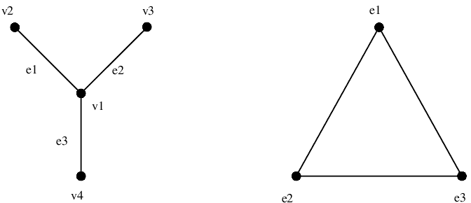
Let us consider the star graph S3S_{3} with a fixed order for the vertices and for the edges, depicted in Fig. 2 on the left. The line graph L⁡(S3)L(S_{3}) is the complete graph K3K_{3} on 33 vertices. Consider the closed walk W=e1,e2,e3,e1W=e_{1},e_{2},e_{3},e_{1} in L⁡(S3)L(S_{3}). Let H∈ℋS3H\in\mathcal{H}_{S_{3}}. Then:

ΨL​(H)​(W)=ΨL​(H)​(e1,e2)​ΨL​(H)​(e2,e3)​ΨL​(H)​(e3,e1)=s2​H1,1−1​H1,2​s2​H1,2−1​H1,3​s2​H1,3−1​H1,1=s2.\begin{split}\Psi_{L}(H)(W)&=\Psi_{L}(H)(e_{1},e_{2})\Psi_{L}(H)(e_{2},e_{3})\Psi_{L}(H)(e_{3},e_{1})\\ &=s_{2}H_{1,1}^{-1}H_{1,2}s_{2}H_{1,2}^{-1}H_{1,3}s_{2}H_{1,3}^{-1}H_{1,1}=s_{2}.\end{split}

Clearly, not every gain function ψ\psi on K3K_{3} satisfies the property ψ⁡(W)=s2\psi(W)=s_{2}, and it follows ΨL​(ℋS3)⊊G⁡(L⁡(S3))\Psi_{L}(\mathcal{H}_{S_{3}})\subsetneq G(L(S_{3})).

Refer to caption
Figure 2. The Star graph S3S_{3} and its line graph L⁡(S3)L(S_{3}).
Definition 4.20.

A gain function ζ∈G⁡(L⁡(Γ))\zeta\in G(L(\Gamma)) is said to be a gain-line function if ζ∈ΨL​(ℋΓ)\zeta\in\Psi_{L}(\mathcal{H}_{\Gamma}). A pair (ψ,ζ)∈G⁡(Γ)×G⁡(L⁡(Γ))(\psi,\zeta)\in G(\Gamma)\times G(L(\Gamma)) is said to be compatible if there exists H∈ℋΓH\in\mathcal{H}_{\Gamma} such that Ψ⁡(H)=ψ\Psi(H)=\psi and ΨL​(H)=ζ\Psi_{L}(H)=\zeta.
A gain function ζ\zeta of L⁡(Γ)L(\Gamma) is a gain-line function compatible with a given ψ∈G⁡(Γ)\psi\in G(\Gamma) if the pair (ψ,ζ)(\psi,\zeta) is compatible.
Finally a gain graph (L,ζ)(L,\zeta) is said to be a gain-line graph if there exist a graph Γ\Gamma and a GG-phase H∈ℋΓH\in\mathcal{H}_{\Gamma} such that L⁡(Γ)=LL(\Gamma)=L and ΨL​(H)=ζ\Psi_{L}(H)=\zeta.

Theorem 4.21.

The orbits of the action ll on ℋΓ\mathcal{H}_{\Gamma} are exactly the fibers of ΨL\Psi_{L}. In other words, for H1,H2∈ℋΓH_{1},H_{2}\in\mathcal{H}_{\Gamma}, one has that H1∼lH2H_{1}\sim_{l}H_{2} if and only if ΨL​(H1)=ΨL​(H2)\Psi_{L}(H_{1})=\Psi_{L}(H_{2}).

Proof.

Suppose H1∼lH2H_{1}\sim_{l}H_{2}. Then Eq. (10) and Lemma 4.17 give

AL⁡(Γ),ΨL​(H1)=AL⁡(Γ),ΨL​(H2),A_{L(\Gamma),\Psi_{L}(H_{1})}=A_{L(\Gamma),\Psi_{L}(H_{2})},

that, by virtue of Remark 3.3, implies ΨL​(H1)=ΨL​(H2)\Psi_{L}(H_{1})=\Psi_{L}(H_{2}).

Vice versa, suppose ΨL​(H1)=ΨL​(H2)\Psi_{L}(H_{1})=\Psi_{L}(H_{2}). This implies that

vk=ei∩ej⟹(H1)k,i−1​(H1)k,j=(H2)k,i−1​(H2)k,jv_{k}=e_{i}\cap e_{j}\implies(H_{1})_{k,i}^{-1}(H_{1})_{k,j}=(H_{2})_{k,i}^{-1}(H_{2})_{k,j}

or, equivalently

(17) vk=ei∩ej⟹(H1)k,j​(H2)k,j−1=(H1)k,i​(H2)k,i−1.v_{k}=e_{i}\cap e_{j}\implies(H_{1})_{k,j}(H_{2})^{-1}_{k,j}=(H_{1})_{k,i}(H_{2})^{-1}_{k,i}.

For every vk∈VΓv_{k}\in V_{\Gamma}, ei∈EΓe_{i}\in E_{\Gamma} such that vk∈eiv_{k}\in e_{i}, we define fk,i:=(H1)k,i​(H2)k,i−1∈Gf_{k,i}:=(H_{1})_{k,i}(H_{2})^{-1}_{k,i}\in G. Observe that the element fk,if_{k,i} does not depend on the particular choice of the edge containing vkv_{k}. In fact, if ei≠eje_{i}\neq e_{j}, vk∈eiv_{k}\in e_{i} and vk∈ejv_{k}\in e_{j}, then vk=ei∩ejv_{k}=e_{i}\cap e_{j}, and then, by Eq. (17), we have fk,i=fk,jf_{k,i}=f_{k,j}. Therefore, we can simply write fkf_{k} instead of fk,if_{k,i}. Let us define f∈Gnf\in G^{n} as f:=(f1−1,…,fn−1)f:=(f_{1}^{-1},\ldots,f_{n}^{-1}). Then we have, for vk∈eiv_{k}\in e_{i},

(l⁡(f,H2))k,i=(f¯∗​H2)k,i=fk​(H2)k,i=(H1)k,i​(H2)k,i−1​(H2)k,i=(H1)k,i.(l(f,H_{2}))_{k,i}=(\underline{f}^{*}H_{2})_{k,i}=f_{k}(H_{2})_{k,i}=(H_{1})_{k,i}(H_{2})^{-1}_{k,i}(H_{2})_{k,i}=(H_{1})_{k,i}.

It follows that l⁡(f,H2)=H1l(f,H_{2})=H_{1} and so H1∼lH2H_{1}\sim_{l}H_{2}. ∎

In the light of Lemma 4.9 and Lemma 4.17, the compatible pairs in G⁡(Γ)×G⁡(L⁡(Γ))G(\Gamma)\times G(L(\Gamma)) are those for which a generalization of Eq. (1) and Eq. (2) holds. In the next section we will investigate the well posedness of our definition with respect to the switching equivalence, that is a crucial issue in the theory of gain graphs. The next corollary shows that compatible pairs are nothing but GG-phases, up to the equivalence relation ∼l∩r\sim_{l\cap r}.

Corollary 4.22.

For H1,H2∈ℋΓH_{1},H_{2}\in\mathcal{H}_{\Gamma}, the following are equivalent:

  1. (1)

    Ψ⁡(H1)=Ψ⁡(H2)\Psi(H_{1})=\Psi(H_{2}) and ΨL​(H1)=ΨL​(H2)\Psi_{L}(H_{1})=\Psi_{L}(H_{2});

  2. (2)

    H1∼l∩rH2H_{1}\sim_{l\cap r}H_{2};

  3. (3)

    there exists (f,g)∈S​tl×r​(H1)(f,g)\in St_{l\times r}(H_{1}) such that H2=f¯∗​H1H_{2}=\underline{f}^{*}H_{1};

  4. (4)

    there exists (f,g)∈S​tl×r​(H1)(f,g)\in St_{l\times r}(H_{1}) such that H2=H1​g¯H_{2}=H_{1}\underline{g}.

Proof.

The equivalence (1)⇔\iff(2) is a consequence of Theorem 4.14 and Theorem 4.21.
(3)⟹\Longrightarrow (2)
Suppose H2=f¯∗​H1H_{2}=\underline{f}^{*}H_{1} (and so H1∼lH2H_{1}\sim_{l}H_{2}), and that there exists g∈Gmg\in G^{m} such that f¯∗​H1​g¯=H1\underline{f}^{*}H_{1}\underline{g}=H_{1}. This implies H2​g¯=H1H_{2}\underline{g}=H_{1}, that is, H1∼rH2H_{1}\sim_{r}H_{2}, and then H1∼l∩rH2H_{1}\sim_{l\cap r}H_{2}.
(2)⟹\Longrightarrow (3)
Let H1∼l∩rH2H_{1}\sim_{l\cap r}H_{2}, so that there exist g∈Gmg\in G^{m} and f∈Gnf\in G^{n} such that

H1=H2​g¯H2=f¯∗​H1.H_{1}=H_{2}\underline{g}\qquad H_{2}=\underline{f}^{*}H_{1}.

Therefore, we have H1=f¯∗​H1​g¯H_{1}=\underline{f}^{*}H_{1}\underline{g}, so that (f,g)∈S​tl×r​(H1)(f,g)\in St_{l\times r}(H_{1}).
(2)⇔\iff(4) The proof is similar to the case (2)⇔\iff(3). ∎

Remark 4.23.

Combining Corollary 4.22 with Proposition 4.6, if GG is abelian, for H1,H2∈ℋΓH_{1},H_{2}\in\mathcal{H}_{\Gamma}, we deduce that Ψ⁡(H1)=Ψ⁡(H2)\Psi(H_{1})=\Psi(H_{2}) and ΨL​(H1)=ΨL​(H2)\Psi_{L}(H_{1})=\Psi_{L}(H_{2}) if and only if there exists g∈Gmg\in G^{m} such that H2=H1​g¯H_{2}=H_{1}\underline{g} with g1=g2=⋯=gmg_{1}=g_{2}=\cdots=g_{m}. By Eq. (6), this is equivalent to the existence of g0∈Gg_{0}\in G such that H1=H2​g0=g0​H2H_{1}=H_{2}g_{0}=g_{0}H_{2}.
In other words, the classes of GG-phases up to multiplication by a “scalar” in GG, are in bijection with the compatible pairs. In particular, for a given gain function ψ\psi of Γ\Gamma, choosing a compatible gain function for the line graph L⁡(Γ)L(\Gamma) is equivalent to choose, up to a scalar multiplication, a GG-phase in Ψ−1​(ψ)\Psi^{-1}(\psi). In the language of [13], when GG is abelian, an oriented GG-gain graph (Γ,ψ,H)(\Gamma,\psi,H), considering HH up to scalar multiplications, is a GG-gain graph (Γ,ψ)(\Gamma,\psi) where a compatible gain ζ\zeta is fixed for L⁡(Γ)L(\Gamma).

4.3. GG-phases, switching equivalence and gain-line graph

We are going to study how the switching equivalence affects our definitions and actions, with the aim to give a well posed definition of line graph.

As a first step, we investigate the relation between the action of an element f∈Gnf\in G^{n} (resp. g∈Gmg\in G^{m}) on ℋΓ\mathcal{H}_{\Gamma} and the switching action of the associated switching function

f:VΓ→G,f⁡(vi)↦fi(resp. ​g:VL⁡(Γ)→G,g⁡(vi)↦gi​)f\colon V_{\Gamma}\to G,\;\;f(v_{i})\mapsto f_{i}\qquad\mbox{(resp.\ }g\colon V_{L(\Gamma)}\to G,\;\;g(v_{i})\mapsto g_{i}\mbox{)}

on G⁡(Γ)G(\Gamma) (resp. on G⁡(L⁡(Γ))G(L(\Gamma))), see Definition 3.1.

Lemma 4.24.

Let H∈ℋΓH\in\mathcal{H}_{\Gamma}, f∈Gnf\in G^{n} and g∈Gmg\in G^{m}. We have:

Ψ⁡(f¯∗​H​g¯)=Ψ​(H)fΨL​(f¯∗​H​g¯)=ΨL​(H)g.\begin{split}\Psi(\underline{f}^{*}H\underline{g})&=\Psi(H)^{f}\\ \Psi_{L}(\underline{f}^{*}H\underline{g})&=\Psi_{L}(H)^{g}.\end{split}
Proof.

Let ek={vi,vj}∈EΓe_{k}=\{v_{i},v_{j}\}\in E_{\Gamma}. Then, by Eq. (11), we have:

Ψ⁡(f¯∗​H​g¯)​(vi,vj)=s1​(f¯∗​H​g¯)i,k​(f¯∗​H​g¯)j,k−1=s1​(fi−1​Hi,k​gk)​(fj−1​Hj,k​gk)−1=s1​fi−1​Hi,k​gk​gk−1​Hj,k−1​fj=fi−1​s1​Hi,k​Hj,k−1​fj=fi−1​Ψ​(H)​(vi,vj)​fj=Ψ​(H)f​(vi,vj).\begin{split}\Psi(\underline{f}^{*}H\underline{g})(v_{i},v_{j})&=s_{1}(\underline{f}^{*}H\underline{g})_{i,k}(\underline{f}^{*}H\underline{g})_{j,k}^{-1}=s_{1}(f_{i}^{-1}H_{i,k}g_{k})(f^{-1}_{j}H_{j,k}g_{k})^{-1}\\ &=s_{1}f_{i}^{-1}H_{i,k}g_{k}g_{k}^{-1}H_{j,k}^{-1}f_{j}=f_{i}^{-1}s_{1}H_{i,k}H_{j,k}^{-1}f_{j}=f_{i}^{-1}\Psi(H)(v_{i},v_{j})f_{j}\\ &=\Psi(H)^{f}(v_{i},v_{j}).\end{split}

Let El={ei,ej}∈EL⁡(Γ)E_{l}=\{e_{i},e_{j}\}\in E_{L(\Gamma)}, vk=ei∩ej∈VΓv_{k}=e_{i}\cap e_{j}\in V_{\Gamma}. Then, by Eq. (15), we have:

ΨL​(f¯∗​H​g¯)​(ei,ej)=s2​(f¯∗​H​g¯)k,i−1​(f¯∗​H​g¯)k,j=s2​(fk−1​Hk,i​gi)−1​(fk−1​Hk,j​gj)=s2​gi−1​Hk,i−1​fk​fk−1​Hk,j​gj=gi−1​s2​Hk,i−1​Hk,j​gj=gi−1​ΨL​(H)​(ei,ej)​gj=ΨL​(H)g​(ei,ej).\begin{split}\Psi_{L}(\underline{f}^{*}H\underline{g})(e_{i},e_{j})&=s_{2}(\underline{f}^{*}H\underline{g})_{k,i}^{-1}(\underline{f}^{*}H\underline{g})_{k,j}=s_{2}(f_{k}^{-1}H_{k,i}g_{i})^{-1}(f_{k}^{-1}H_{k,j}g_{j})\\ &=s_{2}g_{i}^{-1}H_{k,i}^{-1}f_{k}f_{k}^{-1}H_{k,j}g_{j}=g_{i}^{-1}s_{2}H_{k,i}^{-1}H_{k,j}g_{j}=g_{i}^{-1}\Psi_{L}(H)(e_{i},e_{j})g_{j}\\ &=\Psi_{L}(H)^{g}(e_{i},e_{j}).\end{split}

∎

The previous lemma, combined with the results of the previous section, allows us to enunciate one of the main results of the paper.

Theorem 4.25.

The orbits of the action l×rl\times r on ℋΓ\mathcal{H}_{\Gamma} are exactly the subsets Ψ−1​([ψ])\Psi^{-1}([\psi]) or, equivalently, the subsets ΨL−1​([ζ])\Psi_{L}^{-1}([\zeta]). In other words, for H1,H2∈ℋΓH_{1},H_{2}\in\mathcal{H}_{\Gamma}, the following are equivalent:

  1. (1)

    H1∼l×rH2H_{1}\sim_{l\times r}H_{2}

  2. (2)

    Ψ⁡(H1)∼Ψ⁡(H2)\Psi(H_{1})\sim\Psi(H_{2})

  3. (3)

    ΨL​(H1)∼ΨL​(H2).\Psi_{L}(H_{1})\sim\Psi_{L}(H_{2}).

In particular, there exists an injection ℒ:[G⁡(Γ)]→[G⁡(L⁡(Γ))]\mathcal{L}\colon[G(\Gamma)]\to[G(L(\Gamma))], such that ℒ⁡([Ψ⁡(H)])=[ΨL​(H)]\mathcal{L}([\Psi(H)])=[\Psi_{L}(H)], for every H∈ℋΓH\in\mathcal{H}_{\Gamma}.

Proof.


(1)⇔\iff(2)
Suppose H1∼l×rH2H_{1}\sim_{l\times r}H_{2}, so that H2=f¯∗​H1​g¯H_{2}=\underline{f}^{*}H_{1}\underline{g}. By Lemma 4.24 it follows that

Ψ⁡(H2)=Ψ⁡(f¯∗​H1​g¯)=Ψ​(H1)f,\Psi(H_{2})=\Psi(\underline{f}^{*}H_{1}\underline{g})=\Psi(H_{1})^{f},

that is Ψ⁡(H1)∼Ψ⁡(H2)\Psi(H_{1})\sim\Psi(H_{2}).
Vice versa, if Ψ⁡(H2)=Ψ​(H1)f\Psi(H_{2})=\Psi(H_{1})^{f}, we define H0:=f¯∗​H1∈ℋΓH_{0}:=\underline{f}^{*}H_{1}\in\mathcal{H}_{\Gamma}. By Lemma 4.24, we have

Ψ⁡(H0)=Ψ⁡(f¯∗​H1)=Ψ​(H1)f=Ψ⁡(H2).\Psi(H_{0})=\Psi(\underline{f}^{*}H_{1})=\Psi(H_{1})^{f}=\Psi(H_{2}).

By virtue of Theorem 4.14, we have H0∼rH2H_{0}\sim_{r}H_{2}. But we also have, by definition of H0H_{0}, H0∼lH1H_{0}\sim_{l}H_{1}. It follows from Remark 4.7 that H1∼l×rH2H_{1}\sim_{l\times r}H_{2}.
(1)⇔\iff(3)
Suppose H1∼l×rH2H_{1}\sim_{l\times r}H_{2}, so that H2=f¯∗​H1​g¯H_{2}=\underline{f}^{*}H_{1}\underline{g}. By Lemma 4.24 it follows that

ΨL​(H2)=ΨL​(f¯∗​H1​g¯)=ΨL​(H1)g,\Psi_{L}(H_{2})=\Psi_{L}(\underline{f}^{*}H_{1}\underline{g})=\Psi_{L}(H_{1})^{g},

that is ΨL​(H1)∼ΨL​(H2)\Psi_{L}(H_{1})\sim\Psi_{L}(H_{2}).
Vice versa, if ΨL​(H2)=ΨL​(H1)g\Psi_{L}(H_{2})=\Psi_{L}(H_{1})^{g}, we define H0:=H1​g¯∈ℋΓH_{0}:=H_{1}\underline{g}\in\mathcal{H}_{\Gamma}. By Lemma 4.24, we have

ΨL​(H0)=ΨL​(H1​g¯)=ΨL​(H1)g=ΨL​(H2).\Psi_{L}(H_{0})=\Psi_{L}(H_{1}\underline{g})=\Psi_{L}(H_{1})^{g}=\Psi_{L}(H_{2}).

By virtue of Theorem 4.21, we have H0∼lH2H_{0}\sim_{l}H_{2}. But we also have, by definition of H0H_{0}, H0∼rH1H_{0}\sim_{r}H_{1}. It follows from Remark 4.7 that H1∼l×rH2H_{1}\sim_{l\times r}H_{2}. ∎

Corollary 4.26.

Let (ψ,ζ)(\psi,\zeta) be a pair in G⁡(Γ)×G⁡(L⁡(Γ))G(\Gamma)\times G(L(\Gamma)). The following are equivalent:

  1. (1)

    (ψ,ζ)(\psi,\zeta) is compatible;

  2. (2)

    ℒ⁡([ψ])=[ζ]\mathcal{L}([\psi])=[\zeta].

In particular, if (ψ,ζ)(\psi,\zeta) is compatible then (ψ′,ζ′)(\psi^{\prime},\zeta^{\prime}) is compatible for any ψ′∼ψ\psi^{\prime}\sim\psi and any ζ′∼ζ\zeta^{\prime}\sim\zeta.

Proof.

Let (ψ,ζ)=(Ψ⁡(H),ΨL​(H))(\psi,\zeta)=(\Psi(H),\Psi_{L}(H)), for some H∈ℋΓH\in\mathcal{H}_{\Gamma}. By Theorem 4.25 we have [ζ]=[ΨL​(H)]=ℒ⁡([Ψ⁡(H)])=ℒ⁡([ψ])[\zeta]=[\Psi_{L}(H)]=\mathcal{L}([\Psi(H)])=\mathcal{L}([\psi]).
Vice versa, suppose ℒ⁡([ψ])=[ζ]\mathcal{L}([\psi])=[\zeta]. By Proposition 4.13, there exists H∈ℋΓH\in\mathcal{H}_{\Gamma} such that Ψ⁡(H)=ψ\Psi(H)=\psi. Then [ζ]=ℒ⁡([ψ])=ℒ⁡([Ψ⁡(H)])=[ΨL​(H)][\zeta]=\mathcal{L}([\psi])=\mathcal{L}([\Psi(H)])=[\Psi_{L}(H)]. In particular, there exists g∈Gmg\in G^{m} such that ζ=ΨL​(H)g\zeta=\Psi_{L}(H)^{g}. Then (ψ,ζ)=(Ψ⁡(H),ΨL​(H)g)=(Ψ⁡(H​g¯),ΨL​(H​g¯))(\psi,\zeta)=(\Psi(H),\Psi_{L}(H)^{g})=(\Psi(H\underline{g}),\Psi_{L}(H\underline{g})) by Lemma 4.24. ∎

Corollary 4.26 shows that the compatible pairs are exactly all the choices of representatives of [ψ][\psi] and ℒ⁡([ψ])\mathcal{L}([\psi]). In particular, the properties introduced in Definition 4.20, like the property of being gain-line function in G⁡(L⁡(Γ))G(L(\Gamma)) or the property of being compatible in G⁡(Γ)×G⁡(L⁡(Γ))G(\Gamma)\times G(L(\Gamma)), do not depend on the choice of representatives of the switching classes.

Then we can interpret ℒ⁡([ψ])\mathcal{L}([\psi]) as the gain-line graph of [ψ][\psi], and the map ℒ\mathcal{L} is the line graph in the context of gain graphs up to switching equivalence.
Now let NΓ​(G)N_{\Gamma}(G) be the matrix defined in Example 4.2.

Corollary 4.27.

For H∈ℋΓH\in\mathcal{H}_{\Gamma}, the following are equivalent:

  1. (1)

    H∼l×rNΓ(G)H\sim_{l\times r}N_{\Gamma}(G);

  2. (2)

    Ψ⁡(H)∼𝕤𝟙\Psi(H)\sim\mathbb{s_{1}} on Γ\Gamma, that is [Ψ⁡(H)]=[𝕤𝟙][\Psi(H)]=[\mathbb{s_{1}}];

  3. (3)

    ΨL​(H)∼𝕤𝟚\Psi_{L}(H)\sim\mathbb{s_{2}} on L⁡(Γ)L(\Gamma), that is [ΨL​(H)]=[𝕤𝟚][\Psi_{L}(H)]=[\mathbb{s_{2}}].

In particular, with the choice s1=s2=1Gs_{1}=s_{2}=1_{G}, for a compatible pair (ψ,ζ)∈G⁡(Γ)×G⁡(L⁡(Γ))(\psi,\zeta)\in G(\Gamma)\times G(L(\Gamma)) one has that (Γ,ψ)(\Gamma,\psi) is balanced if and only if (L⁡(Γ),ζ)(L(\Gamma),\zeta) is balanced.

Proof.

Notice that, by Definition 4.8, we have Ψ⁡(NΓ​(G))=𝕤𝟙\Psi(N_{\Gamma}(G))=\mathbb{s_{1}} and, by Definition 4.16, we have ΨL​(NΓ​(G))=𝕤𝟚\Psi_{L}(N_{\Gamma}(G))=\mathbb{s_{2}}. Then the equivalences follow from Theorem 4.25. ∎

Remark 4.28.

When G=𝕋4G=\mathbb{T}_{4}, with the choices s1=−1s_{1}=-1 and s2=1s_{2}=1, our Corollary 4.27 implies that the switching equivalence class of the line graph is balanced if and only if the switching equivalence class of the starting graph is antibalanced. This is the content of [2, Theorem 2].
Moreover, when G={±1}G=\{\pm 1\} with s1=s2=−1s_{1}=s_{2}=-1, our Corollary 4.27 implies that the switching equivalence class of the line graph is balanced if and only if the switching equivalence class of the starting graph is balanced, as one can deduce from [21, Section V].

We have seen that the map ℒ:[G⁡(Γ)]→[G⁡(L⁡(Γ))]\mathcal{L}\colon[G(\Gamma)]\to[G(L(\Gamma))] is defined up to switching equivalence. However, paying the price to make a particular choice by fixing an orientation 𝔬\mathfrak{o} of Γ\Gamma, we can lift the map ℒ\mathcal{L} to a map ℒ𝔬:G⁡(Γ)→G⁡(L⁡(Γ))\mathcal{L}_{\mathfrak{o}}\colon G(\Gamma)\to G(L(\Gamma)). This is possible thanks to the map H𝔬H_{\mathfrak{o}}, introduced in Definition 4.11, that in Proposition 4.13 is proved to be a section of Ψ:ℋΓ→G⁡(Γ)\Psi\colon\mathcal{H}_{\Gamma}\to G(\Gamma). By putting ℒ𝔬:=ΨL∘H𝔬\mathcal{L}_{\mathfrak{o}}:=\Psi_{L}\circ H_{\mathfrak{o}} we have that, by Theorem 4.25, the following diagram commutes.

G⁡(Γ){\lx@inpgf@ignorespaces G(\Gamma)}G⁡(L⁡(Γ)){\lx@inpgf@ignorespaces G(L(\Gamma))}[G⁡(Γ)]{\lx@inpgf@ignorespaces\left[G(\Gamma)\right]}[G⁡(L⁡(Γ))]{\lx@inpgf@ignorespaces\left[G(L(\Gamma))\right]}ℒ𝔬\scriptstyle{\lx@inpgf@ignorespaces\mathcal{L}_{\mathfrak{o}}}ℒ\scriptstyle{\lx@inpgf@ignorespaces\mathcal{L}}

For a more complete picture of the relations among these maps see Fig. 5. We are also able to give in Proposition 4.29 an explicit description of the map ℒ𝔬\mathcal{L}_{\mathfrak{o}}. In particular, the rules given in Eq. (18) are represented in Fig. 3.

Proposition 4.29.

Let ψ\psi be a gain function on Γ\Gamma, and let 𝔬\mathfrak{o} be a fixed orientation for its edges. Let ea,eb∈EΓe_{a},e_{b}\in E_{\Gamma} such that ea={v1,v2}e_{a}=\{v_{1},v_{2}\}, eb={v2,v3}e_{b}=\{v_{2},v_{3}\}, so that {ea,eb}∈EL⁡(Γ)\{e_{a},e_{b}\}\in E_{L(\Gamma)}. Then:

(18) ℒ𝔬​(ψ)​(ea,eb)={s1​s2​ψ​(v2,v3) if ​ea𝔬=(v1,v2),eb𝔬=(v2,v3)s2 if ​ea𝔬=(v1,v2),eb𝔬=(v3,v2)s2​ψ​(v1,v2)​ψ​(v2,v3) if e𝔬a=(v2,v1),e𝔬b=(v2,v3).\mathcal{L}_{\mathfrak{o}}(\psi)(e_{a},e_{b})=\begin{cases}s_{1}s_{2}\psi(v_{2},v_{3})&\mbox{ if }e^{\mathfrak{o}}_{a}=(v_{1},v_{2}),e^{\mathfrak{o}}_{b}=(v_{2},v_{3})\\ s_{2}&\mbox{ if }e^{\mathfrak{o}}_{a}=(v_{1},v_{2}),e^{\mathfrak{o}}_{b}=(v_{3},v_{2})\\ s_{2}\psi(v_{1},v_{2})\psi(v_{2},v_{3})&\mbox{ if }e^{\mathfrak{o}}_{a}=(v_{2},v_{1}),e^{\mathfrak{o}}_{b}=(v_{2},v_{3}).\end{cases}
Proof.

For {ea,eb}∈EL⁡(Γ)\{e_{a},e_{b}\}\in E_{L(\Gamma)}, v2=ea∩ebv_{2}=e_{a}\cap e_{b}, by Definition 4.16 we have:

(19) ℒ𝔬​(ψ)​(ea,eb)=ΨL​(H𝔬​(ψ))​(ea,eb)=s2​H𝔬​(ψ)2,a−1​H𝔬​(ψ)2,b.\mathcal{L}_{\mathfrak{o}}(\psi)(e_{a},e_{b})=\Psi_{L}(H_{\mathfrak{o}}(\psi))(e_{a},e_{b})=s_{2}H_{\mathfrak{o}}(\psi)_{2,a}^{-1}H_{\mathfrak{o}}(\psi)_{2,b}.

Since ea={v1,v2}e_{a}=\{v_{1},v_{2}\}, eb={v2,v3}e_{b}=\{v_{2},v_{3}\}, by Definition 4.11 we have:

(20) H𝔬​(ψ)2,a:={ψ⁡(v2,v1) if ​(v2,v1)∈𝔬s1 if ​(v1,v2)∈𝔬H𝔬​(ψ)2,b:={ψ⁡(v2,v3) if ​(v2,v3)∈𝔬s1 if ​(v3,v2)∈𝔬.H_{\mathfrak{o}}(\psi)_{2,a}:=\begin{cases}\psi(v_{2},v_{1})&\mbox{ if }(v_{2},v_{1})\in\mathfrak{o}\\ s_{1}&\mbox{ if }(v_{1},v_{2})\in\mathfrak{o}\end{cases}\quad H_{\mathfrak{o}}(\psi)_{2,b}:=\begin{cases}\psi(v_{2},v_{3})&\mbox{ if }(v_{2},v_{3})\in\mathfrak{o}\\ s_{1}&\mbox{ if }(v_{3},v_{2})\in\mathfrak{o}.\end{cases}

By gluing together Eqs. (19) and (20), we obtain Eq. (18) and the proof is completed. ∎

ψ,𝔬{\lx@inpgf@ignorespaces\psi,\mathfrak{o}}ℒ𝔬​(ψ){\lx@inpgf@ignorespaces\mathcal{L}_{\mathfrak{o}}(\psi)}v1{\lx@inpgf@ignorespaces v_{1}}v2{\lx@inpgf@ignorespaces v_{2}}v3{\lx@inpgf@ignorespaces v_{3}}ea{\lx@inpgf@ignorespaces{e_{a}}}eb{\lx@inpgf@ignorespaces{e_{b}}}v1{\lx@inpgf@ignorespaces v_{1}}v2{\lx@inpgf@ignorespaces v_{2}}v3{\lx@inpgf@ignorespaces v_{3}}ea{\lx@inpgf@ignorespaces{e_{a}}}eb{\lx@inpgf@ignorespaces{e_{b}}}v1{\lx@inpgf@ignorespaces v_{1}}v2{\lx@inpgf@ignorespaces v_{2}}v3{\lx@inpgf@ignorespaces v_{3}}ea{\lx@inpgf@ignorespaces{e_{a}}}eb{\lx@inpgf@ignorespaces{e_{b}}}x\scriptstyle{\lx@inpgf@ignorespaces x}ea𝔬\scriptstyle{\lx@inpgf@ignorespaces e_{a}^{\mathfrak{o}}}y\scriptstyle{\lx@inpgf@ignorespaces y}eb𝔬\scriptstyle{\lx@inpgf@ignorespaces e_{b}^{\mathfrak{o}}}s1​s2​y\scriptstyle{\lx@inpgf@ignorespaces s_{1}s_{2}y}s1​s2​y−1\scriptstyle{\lx@inpgf@ignorespaces s_{1}s_{2}y^{-1}}x\scriptstyle{\lx@inpgf@ignorespaces x}ea𝔬\scriptstyle{\lx@inpgf@ignorespaces e_{a}^{\mathfrak{o}}}y\scriptstyle{\lx@inpgf@ignorespaces y}eb𝔬\scriptstyle{\lx@inpgf@ignorespaces e_{b}^{\mathfrak{o}}}s2\scriptstyle{\lx@inpgf@ignorespaces s_{2}}s2\scriptstyle{\lx@inpgf@ignorespaces s_{2}}x\scriptstyle{\lx@inpgf@ignorespaces x}ea𝔬\scriptstyle{\lx@inpgf@ignorespaces e_{a}^{\mathfrak{o}}}y\scriptstyle{\lx@inpgf@ignorespaces y}eb𝔬\scriptstyle{\lx@inpgf@ignorespaces e_{b}^{\mathfrak{o}}}s2​x−1​y\scriptstyle{\lx@inpgf@ignorespaces s_{2}x^{-1}y}s2​y−1​x\scriptstyle{\lx@inpgf@ignorespaces s_{2}y^{-1}x}
Figure 3. The construction of ℒ𝔬​(ψ)\mathcal{L}_{\mathfrak{o}}(\psi).
Example 4.30.

Consider the Paw graph PP, its ℚ8\mathbb{Q}_{8}-gain function ψ\psi and its orientation 𝔬<\mathfrak{o}_{<} described in Example 4.12, with the choices s1=s2=−1s_{1}=s_{2}=-1. On the left side of Fig. 4 the gain graph (P,ψ)(P,\psi) is depicted with the orientation of the edges given by 𝔬<\mathfrak{o}_{<}. On the right side of Fig. 4 the associated gain-line graph (L​(P),ℒ𝔬<​(ψ))(L(P),\mathcal{L}_{\mathfrak{o}_{<}}(\psi)) is depicted. Notice how the gain function ℒ𝔬<​(ψ)\mathcal{L}_{\mathfrak{o}_{<}}(\psi) can be constructed via the rules described in Fig. 3.

v3v_{3}v4v_{4}v2v_{2}v1v_{1}e1e_{1}e2e_{2}e3e_{3}e4e_{4}−i-ie1𝔬e^{\mathfrak{o}}_{1}−j-je2𝔬e^{\mathfrak{o}}_{2}−k-ke3𝔬e^{\mathfrak{o}}_{3}−i-ie4𝔬e^{\mathfrak{o}}_{4}−j-j−k-k−1-1−i-i−k-k
Figure 4. The gain graph (P,ψ)(P,\psi) and its gain-line graph (L​(P),ℒ𝔬<​(ψ))(L(P),\mathcal{L}_{\mathfrak{o}_{<}}(\psi)) associated with the orientation 𝔬<\mathfrak{o}_{<}.

Observe that, when G={±1}G=\{\pm 1\}, with s1=s2=−1s_{1}=s_{2}=-1, this construction of signed line graphs is consistent, up to switching equivalence, with the one outlined in [21].
Moreover, when G=𝕋4G=\mathbb{T}_{4} with s1=−1s_{1}=-1 and s2=1s_{2}=1, the line 𝕋4\mathbb{T}_{4}-gain graph that we obtain is switching equivalent to that in [2, Eq. (5)].

4.4. Line GG-phased graph

The aim of this section is to compare our definition of line graph with the definition of line graph of an oriented GG-gain graph given in [13]. More precisely, Reff defined a map from the set of GG-phases of Γ\Gamma to the set of GG-phases of L⁡(Γ)L(\Gamma), and he proved that it is well defined with respect to the switching equivalence of the gain functions obtained from the GG-phases (see [13, Theorem 4.2]). We are going to show that our machinery is consistent with that of [13] and generalizes the result of Reff to the nonabelian case.

Recall that L⁡(Γ)=(VL⁡(Γ),EL⁡(Γ))L(\Gamma)=(V_{L(\Gamma)},E_{L(\Gamma)}), with VL⁡(Γ)=EΓV_{L(\Gamma)}=E_{\Gamma} and fix for VL⁡(Γ)V_{L(\Gamma)} the same order of EΓE_{\Gamma}. Suppose |EL⁡(Γ)|=q|E_{L(\Gamma)}|=q and let us fix an order EL⁡(Γ)={E1,…,Eq}E_{L(\Gamma)}=\{E_{1},\ldots,E_{q}\}. For an edge Ek={ei,ej}∈EL⁡(Γ)E_{k}=\{e_{i},e_{j}\}\in E_{L(\Gamma)}, let us set v⁡(Ek):=ei∩ej∈VΓv(E_{k}):=e_{i}\cap e_{j}\in V_{\Gamma}.
Notice that ℋΓ⊆Mn×m​(ℂ​G)\mathcal{H}_{\Gamma}\subseteq M_{n\times m}(\mathbb{C}G) and ℋL⁡(Γ)⊆Mm×q​(ℂ​G)\mathcal{H}_{L(\Gamma)}\subseteq M_{m\times q}(\mathbb{C}G).

Definition 4.31.

Put L:ℋΓ→ℋL⁡(Γ)L\colon\mathcal{H}_{\Gamma}\to\mathcal{H}_{L(\Gamma)} such that

L​(H)i,k={0 if ​ei∉EkHl,i−1 if ei∈Ek,v(Ek)=vl.L(H)_{i,k}=\begin{cases}0&\mbox{ if }e_{i}\notin E_{k}\\ H_{l,i}^{-1}&\mbox{ if }e_{i}\in E_{k},v(E_{k})=v_{l}.\\ \end{cases}

Observe that our Definition 4.31 coincides with the definition given in [13, Eq. (4.1)].
With a given GG-phased graph (Γ,H)(\Gamma,H) we can associate the GG-phased-line graph (L⁡(Γ),L⁡(H))(L(\Gamma),L(H)). Among the results of the next theorem there is that the pair (Ψ⁡(H),s1​s2​Ψ​(L⁡(H)))∈G⁡(Γ)×G⁡(L⁡(Γ))(\Psi(H),s_{1}s_{2}\Psi(L(H)))\in G(\Gamma)\times G(L(\Gamma)) is compatible, or equivalently ℒ⁡([Ψ⁡(H)])=[s1​s2​Ψ​(L⁡(H))]\mathcal{L}([\Psi(H)])=[s_{1}s_{2}\Psi(L(H))].

Theorem 4.32.

For any H∈ℋΓH\in\mathcal{H}_{\Gamma}, for any g∈Gmg\in G^{m}, for any f∈Gnf\in G^{n}, one has:

  1. (1)

    L⁡(H​g¯)=g¯∗​L​(H)L(H\underline{g})=\underline{g}^{*}L(H);

  2. (2)

    L⁡(f¯∗​H)=L⁡(H)​f′¯L(\underline{f}^{*}H)=L(H)\underline{f^{\prime}}, for some f′∈Gqf^{\prime}\in G^{q};

  3. (3)

    ΨL​(H)=s1​s2​Ψ​(L⁡(H))\Psi_{L}(H)=s_{1}s_{2}\Psi(L(H)).

Proof.


(1)
If ei∉Eke_{i}\notin E_{k}, clearly L​(H​g¯)i,k=0=(g¯∗​L​(H))i,kL(H\underline{g})_{i,k}=0=(\underline{g}^{*}L(H))_{i,k}. Now suppose that ei∈Eke_{i}\in E_{k} and v⁡(Ek)=vlv(E_{k})=v_{l}. Then:

L​(H​g¯)i,k=(H​g¯)l,i−1=(Hl,i​gi)−1=gi−1​Hl,i−1=gi−1​L​(H)i,k=(g¯∗​L​(H))i,kL(H\underline{g})_{i,k}=(H\underline{g})_{l,i}^{-1}=(H_{l,i}g_{i})^{-1}=g_{i}^{-1}H_{l,i}^{-1}=g_{i}^{-1}L(H)_{i,k}=(\underline{g}^{*}L(H))_{i,k}

and the thesis follows.
(2)
For every k=1,…,qk=1,\ldots,q, there exists lk∈{1,…,n}l_{k}\in\{1,\ldots,n\} such that v⁡(Ek)=vlkv(E_{k})=v_{l_{k}}. For a given f∈Gnf\in G^{n}, let us define the element f′∈Gqf^{\prime}\in G^{q} such that fk′=flkf^{\prime}_{k}=f_{l_{k}}. If ei∉Eke_{i}\notin E_{k}, clearly L​(f¯​H)i,k=0=(L⁡(H)​f′¯)i,kL(\underline{f}H)_{i,k}=0=(L(H)\underline{f^{\prime}})_{i,k}. Now suppose that ei∈Eke_{i}\in E_{k} and v⁡(Ek)=vlkv(E_{k})=v_{l_{k}}. Then

L​(f¯∗​H)i,k=(f¯∗​H)lk,i−1=(flk−1​Hlk,i)−1=Hlk,i−1​flk=L​(H)i,k​fk′=(L⁡(H)​f′¯)i,kL(\underline{f}^{*}H)_{i,k}=(\underline{f}^{*}H)_{l_{k},i}^{-1}=(f_{l_{k}}^{-1}H_{l_{k},i})^{-1}=H_{l_{k},i}^{-1}f_{l_{k}}=L(H)_{i,k}f^{\prime}_{k}=(L(H)\underline{f^{\prime}})_{i,k}

and the thesis follows.
(3)
From Definition 4.8 we have Ψ⁡(L⁡(H))​(ei,ej)=s1​L​(H)i,k​(L​(H)j,k)−1\Psi(L(H))(e_{i},e_{j})=s_{1}L(H)_{i,k}(L(H)_{j,k})^{-1} with Ek={ei,ej}∈EL⁡(Γ)E_{k}=\{e_{i},e_{j}\}\in E_{L(\Gamma)}. Suppose that vl=ei∩ej∈VΓv_{l}=e_{i}\cap e_{j}\in V_{\Gamma}. Then by Definition 4.31 we have L​(H)i,k=Hl,i−1L(H)_{i,k}=H_{l,i}^{-1} and L​(H)j,k=Hl,j−1L(H)_{j,k}=H_{l,j}^{-1}, so that:

Ψ⁡(L⁡(H))​(ei,ej)=s1​L​(H)i,k​(L​(H)j,k)−1=s1​Hl,i−1​Hl,j.\Psi(L(H))(e_{i},e_{j})=s_{1}L(H)_{i,k}(L(H)_{j,k})^{-1}=s_{1}H_{l,i}^{-1}H_{l,j}.

On the other hand, by Definition 4.16, we also have ΨL​(H)​(ei,ej)=s2​Hl,i−1​Hl,j\Psi_{L}(H)(e_{i},e_{j})=s_{2}H_{l,i}^{-1}H_{l,j} and the thesis follows. ∎

As a consequence, when s1=s2s_{1}=s_{2} and the interest is only in the gain-line graph and not in its GG-phase, considering Ψ⁡(L⁡(H))\Psi(L(H)) or ΨL​(H)\Psi_{L}(H) is equivalent. Under these assumptions, our results in the previous sections can be applied in the context of [13]. More precisely, when GG is abelian with s1=s2s_{1}=s_{2}, Corollary 4.27, combined with Theorem 4.32, generalizes the content of [13, Proposition 4.1]. Moreover Theorem 4.25, combined with Theorem 4.32, gives a generalization of the content of [13, Theorem 4.2]. In particular, we give a complete answer to [13, Question 2].

G⁡(Γ){\lx@inpgf@ignorespaces G(\Gamma)}ℋΓ/∼l∩r{\lx@inpgf@ignorespaces\mathcal{H}_{\Gamma}/\sim_{l\cap r}}[G⁡(Γ)]{\lx@inpgf@ignorespaces\left[G(\Gamma)\right]}ℋΓ/∼r{\lx@inpgf@ignorespaces\mathcal{H}_{\Gamma}/\sim_{r}}G⁡(Γ)×G⁡(L⁡(Γ)){\lx@inpgf@ignorespaces G(\Gamma)\times G(L(\Gamma))}ℋΓ{\lx@inpgf@ignorespaces\mathcal{H}_{\Gamma}}ℋΓ/∼l×r{\lx@inpgf@ignorespaces\mathcal{H}_{\Gamma}/\sim_{l\times r}}ℋΓ/∼l{\lx@inpgf@ignorespaces\mathcal{H}_{\Gamma}/\sim_{l}}ℋL⁡(Γ){\lx@inpgf@ignorespaces\mathcal{H}_{L(\Gamma)}}[G⁡(L⁡(Γ))]{\lx@inpgf@ignorespaces\left[G(L(\Gamma))\right]}G⁡(L⁡(Γ)){\lx@inpgf@ignorespaces G(L(\Gamma))}C​o​r.4.22\scriptstyle{\lx@inpgf@ignorespaces\tiny{}_{Cor.\ref{cor:cap}}}ℒ\scriptstyle{\lx@inpgf@ignorespaces\mathcal{L}}T​h​m.4.25\scriptstyle{\lx@inpgf@ignorespaces\tiny\;\;{}_{Thm.\ref{th:rl}}}Ψ×ΨL\scriptstyle{\lx@inpgf@ignorespaces\Psi\times\Psi_{L}}H𝔬\scriptstyle{\lx@inpgf@ignorespaces\tiny{}_{H_{\mathfrak{o}}}}Ψ\scriptstyle{\lx@inpgf@ignorespaces\Psi}T​h​m.4.14\scriptstyle{\lx@inpgf@ignorespaces\tiny{}_{Thm.\ref{th:r}}}P​r​o​p.4.13\scriptstyle{\lx@inpgf@ignorespaces\tiny{}_{Prop.\ref{prop:sur}}}T​h​m.4.21\scriptstyle{\lx@inpgf@ignorespaces\tiny{}^{{}^{Thm.\ref{th:l}}}}ΨL\scriptstyle{\lx@inpgf@ignorespaces\Psi_{L}}L\scriptstyle{\lx@inpgf@ignorespaces L}T​h​m.4.25\scriptstyle{\lx@inpgf@ignorespaces\tiny{}_{Thm.\ref{th:rl}}}T​h​m.4.25\scriptstyle{\lx@inpgf@ignorespaces\tiny{}_{Thm.\ref{th:rl}}}s1​s2​Ψ\scriptstyle{\lx@inpgf@ignorespaces s_{1}s_{2}\Psi}T​h​m.4.32\scriptstyle{\lx@inpgf@ignorespaces\tiny{}^{{}^{Thm.\ref{prop:line}}}}ℒ𝔬\scriptstyle{\lx@inpgf@ignorespaces\mathcal{L}_{\mathfrak{o}}}
Figure 5. Summary of Section 4.

5. Represented Adjacency, Laplacian and GG-phase matrices

We start this section by recalling some basic definitions about group representations. The interested reader is referred to [8] for further details.
A representation of GG on a vector space VV of dimension kk is a group homomorphism π:G→G​Lk​(V),\pi\colon G\to GL_{k}(V), where G​Lk​(V)GL_{k}(V) is the group of all bijective ℂ\mathbb{\mathbb{C}}-linear maps from VV to itself. Notice that the group G​Lk​(V)GL_{k}(V) can be naturally identified with the group G​Lk​(ℂ)GL_{k}(\mathbb{C}) of all invertible matrices of size kk over ℂ\mathbb{C}. Therefore, with a small abuse of notation, one can denote by π\pi the homomorphism that associates with an element g∈Gg\in G the matrix in G​Lk​(ℂ)GL_{k}(\mathbb{C}) corresponding to π⁡(g)\pi(g). The dimension kk of VV is called the degree of π\pi.
A representation π\pi is said to be unitary if π​(g)∈Uk​(ℂ)\pi(g)\in U_{k}(\mathbb{C}), for each g∈Gg\in G, with Uk​(ℂ)={M∈G​Lk​(ℂ):M−1=M∗}U_{k}(\mathbb{C})=\{M\in GL_{k}(\mathbb{C}):M^{-1}=M^{\ast}\}, where M∗M^{*} denotes the Hermitian transpose of MM; π\pi is said to be faithful if only the neutral element of GG is sent to the identity matrix.
A representation π\pi of GG on VV is said to be irreducible if there is no proper invariant subspace W⊂VW\subset V under the action of GG, that is, there is no WW such that π⁡(g)​w∈W\pi(g)w\in W for any w∈Ww\in W and for any g∈Gg\in G. It is known that each representation π\pi of a group GG can be decomposed into the direct sum of irreducible representations.

For any representation π\pi of GG of degree kk, for any element f∈ℂ​Gf\in\mathbb{C}G, with f=∑x∈Gfx​xf=\sum_{x\in G}f_{x}x, the Fourier transform of ff at the representation π\pi is the matrix f^​(π)∈Mk​(ℂ)\hat{f}(\pi)\in M_{k}(\mathbb{C}) such that:

f^​(π)=∑x∈Gfx​π​(x).\hat{f}(\pi)=\sum_{x\in G}f_{x}\pi(x).

Moreover, with a given A=(Ai​j)∈Mn×m​(ℂ​G)A=(A_{ij})\in M_{n\times m}(\mathbb{C}G), we can associate a matrix A^​(π)∈Mn​k×m​k​(ℂ)\widehat{A}(\pi)\in M_{nk\times mk}(\mathbb{C}), that we can write as a block matrix n×mn\times m of type

(A^​(π)1,1A^​(π)1,2⋯A^​(π)1,mA^​(π)2,1A^​(π)2,2⋯A^​(π)2,m⋮⋮⋱⋮A^​(π)n,1A^​(π)n,2⋯A^​(π)n,m)\left(\begin{array}[]{c|c|c|c}\widehat{A}(\pi)_{1,1}&\widehat{A}(\pi)_{1,2}&\cdots&\widehat{A}(\pi)_{1,m}\\ \hline\cr\widehat{A}(\pi)_{2,1}&\widehat{A}(\pi)_{2,2}&\cdots&\widehat{A}(\pi)_{2,m}\\ \hline\cr\vdots&\vdots&\ddots&\vdots\\ \hline\cr\widehat{A}(\pi)_{n,1}&\widehat{A}(\pi)_{n,2}&\cdots&\widehat{A}(\pi)_{n,m}\end{array}\right)

where the block A^​(π)i,j∈Mk×k​(ℂ)\widehat{A}(\pi)_{i,j}\in M_{k\times k}(\mathbb{C}) is the Fourier transform of Ai,j∈ℂ​GA_{i,j}\in\mathbb{C}G at π\pi.

In particular, starting from the adjacency matrix of a gain graph AΓ,ψ∈Mn×n​(ℂ​G)A_{\Gamma,\psi}\in M_{n\times n}(\mathbb{C}G), the matrix AΓ,ψ^​(π)∈Mn​k×n​k​(ℂ)\widehat{A_{\Gamma,\psi}}(\pi)\in M_{nk\times nk}(\mathbb{C}) is obtained by replacing each entry g∈Gg\in G with the k×kk\times k block given by π⁡(g)\pi(g), and each zero entry with a zero matrix of size kk. The matrix AΓ,ψ^​(π)\widehat{A_{\Gamma,\psi}}(\pi) is the represented adjacency matrix AΓ,ψ^​(π)\widehat{A_{\Gamma,\psi}}(\pi) of the gain graph (Γ,ψ)(\Gamma,\psi) with respect to the representation π\pi.
The represented Laplacian matrix ΔΓ,ψs^​(π)\widehat{\Delta^{s}_{\Gamma,\psi}}(\pi) of the gain graph (Γ,ψ)(\Gamma,\psi) with respect to the representation π\pi is defined in a similar way, starting from ΔΓ,ψs\Delta^{s}_{\Gamma,\psi}.

When the representation is faithful, the matrix AΓ,ψ^​(π)\widehat{A_{\Gamma,\psi}}(\pi) contains all the information about the gain graph (Γ,ψ)(\Gamma,\psi). For example, if the spectrum of AΓ,ψ^​(π)\widehat{A_{\Gamma,\psi}}(\pi) is known, then it is possible to establish whether (Γ,ψ)(\Gamma,\psi) is balanced or not (see [5]).

Given f1,f2∈ℂ​Gf_{1},f_{2}\in\mathbb{C}G and a representation π\pi of GG of degree kk, the following properties hold (see, for example, [8]).

(21) (f1+f2)^​(π)\displaystyle\widehat{(f_{1}+f_{2})}(\pi) =\displaystyle= f1^​(π)+f2^​(π);\displaystyle\widehat{f_{1}}(\pi)+\widehat{f_{2}}(\pi);
(22) f1​f2^​(π)\displaystyle\widehat{f_{1}f_{2}}(\pi) =\displaystyle= f1^​(π)​f2^​(π);\displaystyle\widehat{f_{1}}(\pi)\widehat{f_{2}}(\pi);

moreover, if π\pi is unitary, then

(23) f∗^​(π)=f^​(π)∗for each ​f∈ℂ​G.\widehat{f^{*}}(\pi)=\widehat{f}(\pi)^{*}\qquad\textrm{for each }f\in\mathbb{C}G.
Lemma 5.1.

For every A,B∈Mn×l​(ℂ​G)A,B\in M_{n\times l}(\mathbb{C}G), C∈Ml×m​(ℂ​G)C\in M_{l\times m}(\mathbb{C}G), g∈Gg\in G and for every representation π\pi of GG, one has:

  1. (1)

    (A+B)^​(π)=A^​(π)+B^​(π)\widehat{(A+B)}(\pi)=\widehat{A}(\pi)+\widehat{B}(\pi)

  2. (2)

    A​C^​(π)=A^​(π)​C^​(π)\widehat{AC}(\pi)=\widehat{A}(\pi)\widehat{C}(\pi)

  3. (3)

    g​A^​(π)=(In⊗π⁡(g))​A^​(π)\widehat{gA}(\pi)=(I_{n}\otimes\pi(g))\widehat{A}(\pi)

  4. (4)

    A​g^​(π)=A^​(π)​(Il⊗π⁡(g)).\widehat{Ag}(\pi)=\widehat{A}(\pi)(I_{l}\otimes\pi(g)).

Moreover, if π\pi is unitary, then A∗^​(π)=A^​(π)∗\widehat{A^{*}}(\pi)=\widehat{A}(\pi)^{*}.

Proof.

By Eq. (21) we get the following equation of k×kk\times k blocks:

(A+B)^​(π)i,j=(A+B)i,j^​(π)=(Ai,j+Bi,j)^​(π)=Ai,j^​(π)+Bi,j^​(π)=(A^​(π)+B^​(π))i,j,\widehat{(A+B)}(\pi)_{i,j}=\widehat{(A+B)_{i,j}}(\pi)=\widehat{(A_{i,j}+B_{i,j})}(\pi)=\widehat{A_{i,j}}(\pi)+\widehat{B_{i,j}}(\pi)=(\widehat{A}(\pi)+\widehat{B}(\pi))_{i,j},

and then (1) is proved. By virtue of Eqs. (21) and (22) we have the following equation of k×kk\times k blocks:

A​C^​(π)i,j=(A​C)i,j^​(π)=∑k=1lAi,k​Ck,j^​(π)=∑k=1lAi,k​Ck,j^​(π)=∑k=1lAi,k^​(π)​Ck,j^​(π)=(A^​(π)​C^​(π))i,j,\begin{split}\widehat{AC}(\pi)_{i,j}&=\widehat{(AC)_{i,j}}(\pi)=\widehat{\sum_{k=1}^{l}A_{i,k}C_{k,j}}(\pi)=\sum_{k=1}^{l}\widehat{A_{i,k}C_{k,j}}(\pi)=\sum_{k=1}^{l}\widehat{A_{i,k}}(\pi)\widehat{C_{k,j}}(\pi)\\ &=(\widehat{A}(\pi)\widehat{C}(\pi))_{i,j},\end{split}

and then (2) is proved.
By noticing that g​A=d​i​a​g​(g,…,g)​AgA=diag(g,\ldots,g)A and A​g=A​d​i​a​g​(g,…,g)Ag=A\,diag(g,\ldots,g), combining with d​i​a​g​(g,…,g)^​(π)=(In⊗π⁡(g))\widehat{diag(g,\ldots,g)}(\pi)=(I_{n}\otimes\pi(g)), also (3) and (4) are proved.
Finally, if π\pi is unitary, from Eq. (23) we get the following equation of k×kk\times k blocks:

A∗^​(π)i,j=(A∗)i,j^​(π)=(Aj,i)∗^​(π)=(Aj,i)^​(π)∗=(A^​(π)∗)i,j.\widehat{A^{*}}(\pi)_{i,j}=\widehat{(A^{*})_{i,j}}(\pi)=\widehat{(A_{j,i})^{*}}(\pi)=\widehat{(A_{j,i})}(\pi)^{*}=(\widehat{A}(\pi)^{*})_{i,j}.

∎

In particular, the represented adjacency matrix and the represented Laplacian matrix of a gain graph, with respect to a finite dimensional unitary representation π\pi, are Hermitian matrices, with real spectra.

Definition 5.2.

For a matrix AA we denote by σ⁡(A)\sigma(A) the spectrum of AA, that is, the (multi)set of the eigenvalues of AA. For a GG-gain graph (Γ,ψ)(\Gamma,\psi) and a unitary representation π\pi of GG, the π\pi-spectrum of (Γ,ψ)(\Gamma,\psi) is the spectrum σ​(AΓ,ψ^​(π))\sigma(\widehat{A_{\Gamma,\psi}}(\pi)).

By applying the Fourier transform to both sides of Eqs. (12) and (16), we obtain a represented version of Lemma 4.9 and Lemma 4.17, concerning represented adjacency and Laplacian matrices and the Fourier transform of a GG-phase, that we call represented GG-phase. Notice that, if π0\pi_{0} is the 11-dimensional trivial representation (that is, π0​(g)=1\pi_{0}(g)=1, for every g∈Gg\in G), a represented GG-phase is nothing but the classical incidence matrix NN; in this case, Eqs. (12) and (16) reduce to Eqs. (1) and (2), respectively.

Remark 5.3.

If GG is (a subgroup of) 𝕋\mathbb{T} we always have a canonical isomorphism

πi​d:𝕋⟶U1​(ℂ),\pi_{id}:\mathbb{T}\longrightarrow U_{1}(\mathbb{C}),

associating the 1×11\times 1 matrix (z)(z) with each z∈𝕋z\in\mathbb{T}: in particular, the map πi​d\pi_{id} is a faithful unitary representation of degree 11.
For a 𝕋\mathbb{T}-gain graph (Γ,Ψ)(\Gamma,\Psi), with adjacency matrix AΓ,ψ∈Mn​(ℂ​𝕋)A_{\Gamma,\psi}\in M_{n}(\mathbb{C}\mathbb{T}) and Laplacian matrix ΔΓ,ψs∈Mn​(ℂ​𝕋)\Delta^{s}_{\Gamma,\psi}\in M_{n}(\mathbb{C}\mathbb{T}), the matrices AΓ,ψ^​(πi​d)\widehat{A_{\Gamma,\psi}}(\pi_{id}) and ΔΓ,ψs^​(πi​d)\widehat{\Delta^{s}_{\Gamma,\psi}}(\pi_{id}) correspond to the classical adjacency and (signless) Laplacian matrix of a complex unit gain graph (in the sense of [12]).
When G={±1}G=\{\pm 1\}, a represented GG-phase H^​(πi​d)\widehat{H}(\pi_{id}) (with s1=−1s_{1}=-1) is the incidence matrix (or bidirection) in the sense of [21, Section IV].
When G=𝕋4G=\mathbb{T}_{4} (with s1=−1s_{1}=-1 and s2=1s_{2}=1), the matrix H^​(πi​d)\widehat{H}(\pi_{id}) is the incidence matrix in the sense of [2].
Finally when G=𝕋G=\mathbb{T} (with s1=s2s_{1}=s_{2}), the matrix H^​(πi​d)\widehat{H}(\pi_{id}) is the incidence matrix in the sense of [13, Section 5.1].
For all these reasons, our theory is consistent with (and generalizes) the one in [2, 13, 21].

5.1. Spectral conditions to be a gain-line graph

As we have already observed, the Fourier transform provides a represented version of Lemma 4.17. In this section, we develop our group representation approach in order to obtain some necessary conditions for a gain graph to be a gain-line graph (see Definition 4.20).

Theorem 5.4.

Let H∈ℋΓH\in\mathcal{H}_{\Gamma} and let π\pi be a unitary representation of GG of degree kk. Then:

AL​(Γ),ΨL​(H)^​(π)=(Im⊗π⁡(s2))​(H^​(π)∗​H^​(π)−2​Ik​m).\widehat{A_{L(\Gamma),\Psi_{L}(H)}}(\pi)=\ \left(I_{m}\otimes\pi(s_{2})\right)\left(\widehat{H}(\pi)^{*}\widehat{H}(\pi)-2I_{km}\right).
Proof.

By Lemma 4.17 we have: s2​AL​(Γ),ΨL​(H)=H∗​H−2⋅1Gm¯s_{2}A_{L(\Gamma),\Psi_{L}(H)}=H^{*}H-2\cdot\underline{1_{G^{m}}}. Then Lemma 5.1 implies:

(Im⊗π⁡(s2))​AL​(Γ),ΨL​(H)^​(π)\displaystyle\left(I_{m}\otimes\pi(s_{2})\right)\widehat{A_{L(\Gamma),\Psi_{L}(H)}}(\pi) =\displaystyle= (s2​AL​(Γ),ΨL​(H))^​(π)=(H∗​H−2⋅1Gm¯)^​(π)\displaystyle\widehat{(s_{2}A_{L(\Gamma),\Psi_{L}(H)})}(\pi)=\widehat{(H^{*}H-2\cdot\underline{1_{G^{m}}})}(\pi)
=\displaystyle= H^​(π)∗​H^​(π)−2​Ik​m.\displaystyle\widehat{H}(\pi)^{*}\widehat{H}(\pi)-2I_{km}.

We conclude by using the fact that (Im⊗π⁡(s2))−1=Im⊗π⁡(s2)(I_{m}\otimes\pi(s_{2}))^{-1}=I_{m}\otimes\pi(s_{2}) since s2s_{2} is an involution. ∎

Let π\pi be an irreducible representation of degree kk. Since s2s_{2} is central, as a consequence of the Schur’s Lemma (see [8]), the matrix π⁡(s2)\pi(s_{2}) is a scalar matrix. Moreover, it must be π​(s2)2=Ik\pi(s_{2})^{2}=I_{k}, since s2s_{2} is an involution. This implies that either π⁡(s2)=Ik\pi(s_{2})=I_{k} or π⁡(s2)=−Ik\pi(s_{2})=-I_{k}. The two cases are treated in Corollary 5.5 and Corollary 5.6, respectively.

Corollary 5.5.

Let π\pi be a unitary representation of GG of degree kk such that π⁡(s2)=Ik\pi(s_{2})=I_{k}. Then, for every H∈ℋΓH\in\mathcal{H}_{\Gamma}:

σ(AL​(Γ),ΨL​(H)^(π))⊆[−2,∞).\sigma(\widehat{A_{L(\Gamma),\Psi_{L}(H)}}(\pi))\subseteq[-2,\infty).

In particular, if s2=1Gs_{2}=1_{G}, the π\pi-spectrum of a gain-line graph is contained in [−2,∞)[-2,\infty) for any unitary representation π\pi.

Proof.

From Theorem 5.4 we have AL​(Γ),ΨL​(H)^​(π)=H^​(π)∗​H^​(π)−2​Ik​m\widehat{A_{L(\Gamma),\Psi_{L}(H)}}(\pi)=\widehat{H}(\pi)^{*}\widehat{H}(\pi)-2I_{km} and then

σ⁡(AL​(Γ),ΨL​(H)^​(π))=σ⁡(H^​(π)∗​H^​(π))−2.\sigma(\widehat{A_{L(\Gamma),\Psi_{L}(H)}}(\pi))=\sigma(\widehat{H}(\pi)^{*}\widehat{H}(\pi))-2.

The thesis follows since the matrix H^​(π)∗​H^​(π)\widehat{H}(\pi)^{*}\widehat{H}(\pi) is positive semidefinite. ∎

Corollary 5.6.

Let π\pi be a unitary representation of GG of degree kk such that π⁡(s2)=−Ik\pi(s_{2})=-I_{k}. Then, for every H∈ℋΓH\in\mathcal{H}_{\Gamma}:

σ(AL​(Γ),ΨL​(H)^(π))⊆(−∞,2].\sigma(\widehat{A_{L(\Gamma),\Psi_{L}(H)}}(\pi))\subseteq(-\infty,2].
Proof.

From Theorem 5.4 we have AL​(Γ),ΨL​(H)^​(π)=−H^​(π)∗​H^​(π)+2​Ik​m\widehat{A_{L(\Gamma),\Psi_{L}(H)}}(\pi)=-\widehat{H}(\pi)^{*}\widehat{H}(\pi)+2I_{km} and then

σ⁡(AL​(Γ),ΨL​(H)^​(π))=−σ⁡(H^​(π)∗​H^​(π))+2.\sigma(\widehat{A_{L(\Gamma),\Psi_{L}(H)}}(\pi))=-\sigma(\widehat{H}(\pi)^{*}\widehat{H}(\pi))+2.

The thesis follows since the matrix H^​(π)∗​H^​(π)\widehat{H}(\pi)^{*}\widehat{H}(\pi) is positive semidefinite. ∎

As we observed in Remark 5.3, when G=𝕋G=\mathbb{T} the classical spectrum of a 𝕋\mathbb{T}-gain graph is exactly its πi​d\pi_{id}-spectrum. When s2=1s_{2}=1 clearly we have πi​d​(s2)=1\pi_{id}(s_{2})=1 and our Corollary 5.5 generalizes [13, Theorem 5.5]. When s2=−1s_{2}=-1 clearly we have πi​d​(s2)=−1\pi_{id}(s_{2})=-1 and our Corollary 5.6 generalizes [13, Theorem 5.4].

Corollary 5.7.

Let π\pi be a unitary irreducible representation of GG. A GG-gain graph whose π\pi-spectrum contains eigenvalues less than −2-2 and eigenvalues greater than 22 cannot be a gain-line graph, whatever the choice of s2s_{2} is.

In the next example, we show that the conditions obtained in the previous corollaries are not trivial, even if we assume that the underlying graph is a line graph.

Example 5.8.

Let G=ℚ8G=\mathbb{Q}_{8} and consider its (unitary and irreducible) representation π\pi in Table 1.

±1\pm 1 ±i\pm i ±j\pm j ±k\pm k
±(1001)\pm\left(\begin{array}[]{cc}1&0\\ 0&1\\ \end{array}\right) ±(0−110)\pm\left(\begin{array}[]{cc}0&-1\\ 1&0\\ \end{array}\right) ±(0ii0)\pm\left(\begin{array}[]{cc}0&i\\ i&0\\ \end{array}\right) ±(−i00i)\pm\left(\begin{array}[]{cc}-i&0\\ 0&i\\ \end{array}\right)
Table 1. The representation π\pi of ℚ8\mathbb{Q}_{8} of Example 5.8.

Let (Γ,ψ)(\Gamma,\psi) be the gain graph represented in Fig. 6.

v1v_{1}v2v_{2}v3v_{3}v4v_{4}kk1ℚ81_{\mathbb{Q}_{8}}1ℚ81_{\mathbb{Q}_{8}}1ℚ81_{\mathbb{Q}_{8}}jj
Figure 6. The ℚ8\mathbb{Q}_{8}-gain graph (Γ,ψ)(\Gamma,\psi).

We have:

AΓ,ψ=(0−k01k011010−j11j0);AΓ,ψ^​(π)=(00i00010000−i0001−i00010100i0001010010000−i000100−i010100i000101i000).A_{\Gamma,\psi}=\left(\begin{array}[]{cccc}0&-k&0&1\\ k&0&1&1\\ 0&1&0&-j\\ 1&1&j&0\\ \end{array}\right);\qquad\widehat{A_{\Gamma,\psi}}(\pi)=\left(\begin{array}[]{cccccccc}0&0&i&0&0&0&1&0\\ 0&0&0&-i&0&0&0&1\\ -i&0&0&0&1&0&1&0\\ 0&i&0&0&0&1&0&1\\ 0&0&1&0&0&0&0&-i\\ 0&0&0&1&0&0&-i&0\\ 1&0&1&0&0&i&0&0\\ 0&1&0&1&i&0&0&0\\ \end{array}\right).

An explicit computation gives σ⁡(AΓ,ψ^​(π))={(±12​10±2​17)(2)}\sigma(\widehat{A_{\Gamma,\psi}}(\pi))=\left\{\left(\pm\frac{1}{2}\sqrt{10\pm 2\sqrt{17}}\right)^{(2)}\right\}, where the exponent of each eigenvalue denotes its multiplicity. Since 12​10+2​17∼2.135779\frac{1}{2}\sqrt{10+2\sqrt{17}}\sim 2.135779, we have:

σ⁡(AΓ,ψ^​(π))∩(−∞,−2)≠∅ and σ⁡(AΓ,ψ^​(π))∩(+2,∞)≠∅.\sigma(\widehat{A_{\Gamma,\psi}}(\pi))\cap(-\infty,-2)\neq\emptyset\quad\mbox{ and }\quad\sigma(\widehat{A_{\Gamma,\psi}}(\pi))\cap(+2,\infty)\neq\emptyset.

As a consequence of Corollary 5.7, the gain graph (Γ,ψ)(\Gamma,\psi) cannot be a gain-line graph, neither for s2=1s_{2}=1 nor for s2=−1s_{2}=-1, although the underlying graph Γ\Gamma is the line graph of the Paw graph.

References

  • [1] B. D. Acharya, Spectral criterion for cycle balance in networks, J. Graph Theory 4 (1980), no. 1, 1–11.
  • [2] A. Alazemi, M. Anđelić, F. Belardo, M. Brunetti, C. M. da Fonseca, Line and Subdivision Graphs Determined by T4-Gain Graphs, Mathematics 7 (2019), no. 10, 926.
  • [3] F. Belardo, M. Brunetti, N. Reff, Balancedness and the least Laplacian eigenvalue of some complex unit gain graphs, Discuss. Math. Graph Theory 40 (2020), no. 2, 417–433.
  • [4] F. Belardo, S. Simić, On the Laplacian coefficients of signed graphs, Linear Algebra Appl. 475 (2015), 94–113.
  • [5] M. Cavaleri, D. D’Angeli, A. Donno, A group representation approach to balance of gain graphs, submitted, arXiv:2001.08490 (2020).
  • [6] D. Cvetković, P. Rowlinson, S. Simić, An Introduction to the Theory of Graph Spectra, London Mathematical Society Student Texts, 75, Cambridge University Press, Cambridge, 2010, xii + 364 pp.
  • [7] J. Edmonds, E. L. Johnson, Matching: a well-solved class of integer linear programs, Combinatorial optimization - Eureka, you shrink!, 27–30, Lecture Notes in Comput. Sci., 2570, Springer, Berlin, 2003.
  • [8] W. Fulton, J. Harris, Representation theory. A first course. Graduate Texts in Mathematics, 129, Readings in Mathematics, Springer-Verlag, New York, 1991, xvi + 551 pp.
  • [9] F. Harary, Graph theory, Addison-Wesley Publishing Co., Reading, Mass.-Menlo Park, Calif.-London, 1969, ix + 274 pp.
  • [10] R. Mehatari, M. R. Kannan, A. Samanta, On the adjacency matrix of a complex unit gain graph, arXiv:1812.03747 (2018).
  • [11] R. Merris, Laplacian matrices of graphs: a survey, Second Conference of the International, Linear Algebra Society (ILAS) (Lisbon, 1992), Linear Algebra Appl. 197/198 (1994), 143–176.
  • [12] N. Reff, Spectral properties of complex unit gain graphs, Linear Algebra Appl. 436 (2012), no. 9, 3165–3176.
  • [13] N. Reff, Oriented gain graphs, line graphs and eigenvalues, Linear Algebra Appl. 506 (2016), 316–328.
  • [14] K. Shahul Hameed, K.A. Germina, Balance in gain graphs – a spectral analysis, Linear Algebra Appl. 436 (2012), no. 5, 1114–1121.
  • [15] T. Zaslavsky, Signed graphs, Discrete Appl. Math. 4 (1982), no. 1, 47–74.
  • [16] T. Zaslavsky, Biased graphs. I. Bias, balance, and gains, J. Combin. Theory Ser. B 47 (1989), no. 1, 32–52.
  • [17] T. Zaslavsky, Orientation of Signed Graphs, European J. Combin. 12 (1991), no. 4, 361–375.
  • [18] T. Zaslavsky, Glossary of signed and gain graphs and allied areas, Electron. J. Combin. 5 (1998), Dynamic Surveys 9, 41 pp.
  • [19] T. Zaslavsky, A mathematical bibliography of signed and gain graphs and allied areas, Manuscript prepared with Marge Pratt, Electron. J. Combin. 5 (1998), Dynamic Surveys 8, 124 pp.
  • [20] T. Zaslavsky, Biased graphs. IV. Geometrical realizations, J. Combin. Theory Ser. B 89 (2003), no. 2, 231–297.
  • [21] T. Zaslavsky, Matrices in the theory of signed simple graphs, Advances in discrete mathematics and applications: Mysore, 2008, 207–229, Ramanujan Math. Soc. Lect. Notes Ser., 13, Ramanujan Math. Soc., Mysore, 2010.