A regularized deep matrix factorized model of matrix completion for image restoration
Abstract
It has been an important approach of using matrix completion to perform image restoration. Most previous works on matrix completion focus on the low-rank property by imposing explicit constraints on the recovered matrix, such as the constraint of the nuclear norm or limiting the dimension of the matrix factorization component. Recently, theoretical works suggest that deep linear neural network has an implicit bias towards low rank on matrix completion. However, low rank is not adequate to reflect the intrinsic characteristics of a natural image. Thus, algorithms with only the constraint of low rank are insufficient to perform image restoration well. In this work, we propose a Regularized Deep Matrix Factorized (RDMF) model for image restoration, which utilizes the implicit bias of the low rank of deep neural networks and the explicit bias of total variation. We demonstrate the effectiveness of our RDMF model with extensive experiments, in which our method surpasses the state of art models in common examples, especially for the restoration from very few observations. Our work sheds light on a more general framework for solving other inverse problems by combining the implicit bias of deep learning with explicit regularization.
Keywords Total Variation Deep matrix factorization Implicit regularization Explict constraints
1 Introduction
Image restoration from a partially observed pixel is an important problem. An image is often represented by a matrix. Therefore, image restoration is also a matrix completion, that is, recovering unknown or missing entries in a matrix. In addition to image restoration [1, 2, 3], matrix completion problem has a wide spectrum of application venues such as phase recovery [4] and recommendation systems [5, 6]. The prior of low rank has been well studied, and a series of algorithms are developed to well perform matrix completion for low-rank matrices. These algorithms can be classified into two types. The first type imposes explicit constraints on the recovered matrix, such as the constraint of the nuclear norm or limiting the dimension of the matrix factorization component. Such explicit constraints are proved to be successful in many problems [7, 8, 9, 10]. The second type utilizes implicit bias of algorithms. Such implicit bias is recently studied in a deep linear neural network, in theory, i.e., theoretical works suggest that deep linear neural network has an implicit bias towards low rank on matrix completion [11, 12]. However, it is yet to examine its effectiveness in the real application. Low-rank matrix completion has been used in image restoration, while low rank is not adequate to reflect the intrinsic characteristics of a natural image. For example, a restored image with a lower rank can significantly differ with the corresponding intact image. Therefore, it is important to design an algorithm that takes advantage of the study of low-rank matrix completion and preserves the intrinsic properties of a natural image.
In this paper, we design a Regularized Deep Matrix Factorized (RDMF) model to perform the specific matrix completion, that is, image restoration. The idea of this RDMF model is combining a deep neural network with a total variation (TV) regularization. To demonstrate the effectiveness of our model, we compare our model with three representative methods for the restoration of two classic images, i.e., Cameraman and textual image. The first method is a popular linear method, i.e., LaMFit [8]. The second method is also deep matrix factorization (DMF) without TV constraint [10]. The third method is a patch-based nonlinear matrix completion (PNMC) algorithm for the image, which is recently proposed and compared with other methods in [13]. We demonstrate the effectiveness of our RDMF model with extensive experiments, in which our method surpasses these three models in common examples. The restorations of LaMFit and DMF indeed satisfy the low-rank requirement. However, their results have many vertical and horizontal lines, which significantly different from natural images. The result of PNMC shows much more noise. The advantage of our model is significant for the restoration from very few observations. In our experiments, we found that to achieve a good result, the depth of the deep neural network should be larger than two, and the width should be at least around the image size. These results indicate the implicit bias in deep networks with TV better reflects the characteristics of a natural image. In addition, we found that in our model, both deep linear neural networks and nonlinear neural networks have similar good performance, namely, in such image restoration, the benefit from the non-linearity may be incremental.
The remainder of this paper is organized as follows: in Section 2, we give the RDMF model firstly, and then we introduce gradient descent algorithm. In Section 3, we design several experiments to illustrate the critical components of RDMF. In Section 4, we discuss the underlying mechanism of the RDMF. In Section 5, we state conclusions and future research plans.
2 Model formulation
In this section, we mainly discuss how to build gradient descent based matrix completion models.
2.1 Regularized deep matrix factorized model
Before building the model, here we give some more notations, which are slightly different from the suggested notations for machine learning [14]. An -layer neural network is denoted by
| (1) |
where , is a scalar function and "" means entry-wise operation. We denote the vector of all parameters by
and an entry of by .
Assume that the original data matrix without missing entry is . The -th entry of is . The mask matrix is defined as
And the fidelity term for completing by is
| (2) |
where is a dimensions identity matrix, stands for the Hadamard (entry-wise) product.
A regularized model is to solve the following problem:
| (3) |
where is the regularization term. Given some observation , the matrix completion problem can be solved by
When we set , the formulation of the deep network is same as
| (4) |
where is the recovered matrix.
Note that DMF in [10] share same columns in and set . DMF is most similar to our model, but their model requires to constraint the rank of explicitly. Our model do not constraint on the dimension of , as Arora et al. [12] illustrate that Eq. (4) implicitly convergence to low rank matrix. A more important difference between DMF and RDMF is that we set regularization term as TV which will be introduced next section.
The TV regularization is often used in image processing, which tends to a smooth output [15]. The TV norm can either be the anisotropic TV norm
or the isotropic TV norm
where the finite differences and . Note that the anisotropic (isotropic) TV norm is equivalent to discretization of the 1-norm (2-norm) of . They are TV-L1 and TV-L2 respectively in this paper.
We propose our RDMF model as follow:
| (5) |
Compared with TV-L2, the TV-L1 norm leads to a sharper edge. In the noisy image recover problem, 1-norm TV norm is often chosen. However, in the matrix completion problem, we find out that TV-L2 outperformed TV-L1 in most tasks. Without loss of generality, we consider TV regularizer both including TV-L1 and TV-L2.
2.2 Gradient descent
We introduce gradient descent method firstly to build an intuitive understanding of the optimization progress. At time step , the parameters update as follow:
where is the value of parameters at the th iteration, is the learning rate. The vanilla gradient descent algorithm has many drawbacks such as convergence speed is slow and easy to fall into the local optimal. As a result, many variants of gradient descent are proposed to improve the gradient descent algorithm. Adam [16] is one of them and performs well in practical training tasks. Therefore, we choose the Adam algorithm to solve our proposed model 5.
3 Experiment
In this section, we first show the effectiveness of RDMF over peer methods.
3.1 Settings
Task We compare RDMF with LaMFit [8], DMF [10] and PNMC [13] both on natural and textual images. Similar to the tests in [13], all of these images are gray-scale images scaled from standard images. We generate a mask matrix with different missing percentage randomly.
Peer methods
- 1.
LaMFit [8]: Based on the matrix decomposition model, LaMFit constructs a super-relaxation algorithm, which only needs to solve a least-squares problem in each iteration and avoids the the computation consuming SVD in the kernel-norm based method.
- 2.
DMF [10]: This algorithm utilizes deep neural network to recover missing entries without considering regularization.
- 3.
PNMC [13]: Considering the spatial locality of the datasets, convolutional neural network (CNN) is designed to obtain the matrix with missing entries.
- 4.
RDMF: The method proposed in this paper. We default choose TV as regularization term and .
Criteria In order to evaluate the accuracy of the matrix completion, we adopt Normalized Mean Absolute Error (NMAE) [8] as a criteria. NMAE is defined as
where and denote the prediction matrix, the original matrix, the mask matrix of test datasets, the cardinality of , the maximum entry of matrix and the minimum entry of matrix , respectively. Smaller values of NMAE indicate better predictive accuracy than the larger one.
Model parameters settings The hyper-parameters for the proposed method are set as follows: , parameters initialization Gaussian distribution of . Without special instruction, we default set . The algorithm stop when iteration step is larger than 10000 or the training loss , where is the value of at -th iteration. Besides, the proposed algorithm is implemented in the Pytorch framework. All the simulations are conducted on the same workstation with an Intel(R) Xeon(R) Silver 4110 CPU @ 2.10GHz, Nvidia GeForce GRX 2080Ti, running with Linux and using Python tool.
3.2 Effectiveness of RDMF
Firstly we randomly drop pixels in Cameraman and textual image, and then recover them by LaMFit [8], DMF [10], PNMC [13]. Fig. 1 shows the recovered result of different methods. We can observe that both DMF and PNMC perform better than LaMFit. In [10, 13], Fan et al. and Yang et al. claim that the improvement of recovering is derived from the nonlinearity of the model. However, in this experiment, we choose as the activation function of RDMF model, which is degenerate to a linear model. The restored image is much better than all of these models. This indicates that nonlinearity is not always important in image restoration. As shown in Fig. 1 (e), RDMF recover more details than PNMC. Specially, we can identify the text on the recovered result of the textual image. These results illustrate that a linear model with the TV regularization term can well perform the image restoration, even better for a non-linear model.
To explore the effectiveness of the RDMF model, we calculate the NMAE of three peer methods and RDMF with different activation functions. Both of the RDMF with and without TV regularization terms are calculated. Fig. 2 shows the NMAE of restored Cameraman at different missing percentage and models. Tab. 1 shows the NMAE of the restored textual image at different missing percentage and models. We observe that almost all the RDMF model with TV regularization have a lower NMAE than PNMC. Even the linear model of RDMF with TV regularization outperforms other methods. The linear model of RDMF with TV regularization is very similar to the nonlinear one. Note that LaMFit performs better than RDMF of Tanh and ReLU activation function without TV regularization term. Therefore, TV regularization is very important in this image restoration.

| Without TV | With TV | ||||||||||
|---|---|---|---|---|---|---|---|---|---|---|---|
| LaMFit | DMF | PNMC | Proposed | ||||||||
| [8] | [10] | [13] | Linear | ReLU | Sigmoid | Tanh | Linear | ReLU | Sigmoid | Tanh | |
| 30% | 0.0942 | 0.0593 | 0.0454 | 0.0459 | 0.044 | 0.0097 | 0.0249 | 0.0088 | 0.0153 | 0.0083 | 0.009 |
| 40% | 0.0969 | 0.0665 | 0.0531 | 0.0651 | 0.0526 | 0.0122 | 0.0327 | 0.0102 | 0.0243 | 0.0093 | 0.0091 |
| 50% | 0.0975 | 0.0778 | 0.0562 | 0.0851 | 0.0616 | 0.018 | 0.0437 | 0.012 | 0.0116 | 0.0104 | 0.0106 |
| 60% | 0.0998 | 0.0928 | 0.0608 | 0.1115 | 0.0859 | 0.0265 | 0.0593 | 0.0142 | 0.072 | 0.0126 | 0.013 |
| 70% | 0.1036 | 0.1112 | 0.0778 | 0.1485 | 0.118 | 0.0405 | 0.075 | 0.0179 | 0.0617 | 0.0159 | 0.0168 |
| 80% | 0.1148 | 0.1436 | 0.1068 | 0.2154 | 0.1485 | 0.065 | 0.1 | 0.0263 | 0.0871 | 0.0227 | 0.0237 |
| 90% | 0.1462 | 0.165 | 0.1198 | 0.438 | 0.1992 | 0.0991 | 0.1329 | 0.0474 | 0.1308 | 0.0392 | 0.0414 |
| 95% | 0.1605 | 0.1804 | 0.1334 | 0.7105 | 0.2329 | 0.1233 | 0.186 | 0.0751 | 0.156 | 0.0578 | 0.0645 |
| 99% | 0.3586 | 0.2663 | 0.1357 | 0.8729 | 0.4635 | 0.1925 | 0.856 | 0.1343 | 0.6995 | 0.1023 | 0.1178 |
3.3 Wider is better
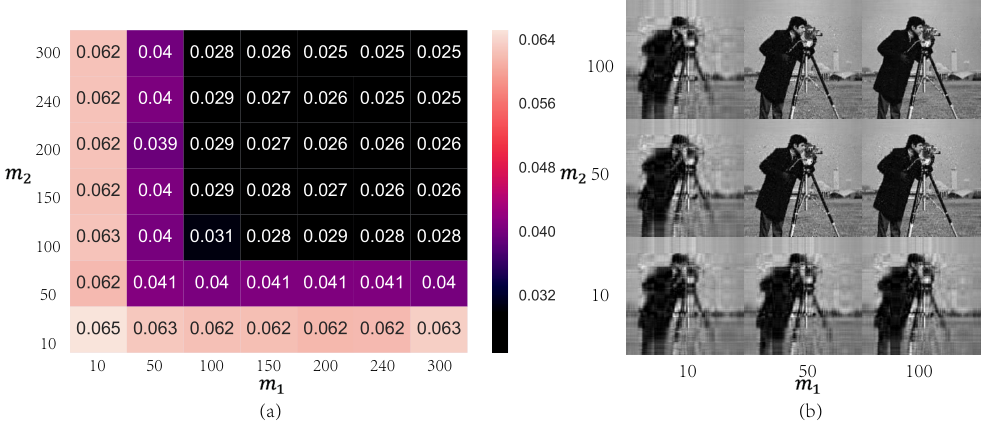
Different from LaMFit and DMF, which constrain small and to ensure the low-rank property of the restored images. We default choose in the before mentioned experiments. Arora et al. [12] claim that when using gradient descent to optimize the loss function (2). The recovered matrix implicitly tends to be low-rank. This implicit low-rank regularization makes our model work with the large and possible. In general, a wider neural network has a stronger express ability. It is reasonable to expect a larger and will lead to better performance. The cameraman of missing pixels with RDMF is restored in this experiment. Fig. 3 shows the NMAE with different and . A larger dimension indeed lead to a better performance on both numerically indicators (Fig. 3(a)) and visually quality (Fig. 3(b)). These results illustrate that the wider neural network can capture more information than a narrower one.
When , the NMAE achieves least. Continue increasing and , RDMF performs same as the case of . In LaMFit and DMF, a proper low dimension is essential for the restored performance. This assumption means that different problems have a different optimal dimension. In RDMF, we choose , and need not worry about a large dimension that will lead to a bad performance.
4 Discussion
According to the numerical results, TV regularization term plays a quite important role in image restoration problems. Intuitively, TV regularization term forces the reconstructed image to have the smoothness property. However, the influence of TV on the implicit low-rank regularization is still unknown. In this section, we follow Arora et al. [12] to obtain an explicitly expression for the dynamics of singular values of the product matrix for our model with a specific regularization term.
To make the statements clear, we still use notations in Section 2 and introduce the following assumption.
Assumption 1.
Factor matrices are balanced at initialization, i.e.,
Under the above assumption, Arora et al. studied the gradient flow of product matrix with the non-regularized risk function , i.e.,
| (6) |
where . The empirical risk can be any analytic function of entries of the matrices, not necessarily the Frobenious norm. Thanks to the analyticity of , we have the following singular value decomposition where each matrix is an analytic function of time.
Lemma 1 ([12]).
The product matrix can be expressed as:
where , and are analytic functions of t; and for every t, the matrices and have orthonormal columns, while is diagonal (its diagonal entries may be negative and may appear in any order).
The diagonal entries of which we denote by are signed singular values of . The columns of and , denoted by and are the corresponding left and right singular vectors respectively.
Proposition 1 ([12, Theorem 3]).
If the matrix factorization is non-degenerate, i.e., has depth the singular values need not be signed (we may assume for all ).
Arora et al. claimed the terms enhance the movement of large singular values, and on the other hand, attenuate that of small ones. The enhancement/attenuation becomes more significant as grows.
This explanation of the implicit low-rank regularization of gradient descent is far from complete because the terms are unkonwn. Hence Arora et al. further discussed a particular case to illustrate the low-rank regularization further. In this paper, we give an illustration of the implicit low-rank regularization of TV-like regularization term. To simplify the proof, we modify from to . The new TV-like regularization term has a negligible influence in experiments. Without loss of generality, we assume , and then we have the following proposition.
Proposition 2.
Consider the following dynamics with initial data satisfying Assumption 1:
where with , and . Then we have
| (8) |
where .
Proof.
This is proved by direct calculation:
Note that
Therefore
where the term . ∎
Corollary 1.
In the setting of Proposition 2, we further have
The terms have a larger exponent than . The terms can enhance/attenuate singular values more significantly than . Specially, if we choose a large enough , is dominated by . The term if and only if all the entries of have the same value, and the rank of equals or . This is consistent with the above analysis. Our theoretic discussion is not complete because both the terms and are unknown and the regularization term is not the exact TV norm. We design some experiments to show our conclusion about the low-rank regularization property of (the exact) TV norm in general.
We calculate the effective rank [17] of RDMF with different activation functions. Both of the RDMF with and without TV regularization terms are calculated. Fig. 4 shows the effective rank of restored Cameraman at different missing percentage and various RDMF. Tab. 2 shows the effective rank of the restored textual image at different missing percentage by different RDMF. Almost all the models with TV have a lower effective rank than these models without TV. This phenomenon is consistent with Corollary 1: TV norm has a stronger implicit low-rank regularization during training. Another important phenomenon is that almost all the models which achieve good performances (Fig. 2, Tab. 1) have a low effective rank. This phenomenon indicates that the implicit low-rank regularization indeed produces better-restored quality. Last but not least, the model with a nonlinear activation function also keeps the restored matrix’s low-rank property. This phenomenon still does not have theoretical analysis, and it needs further research in the future.
Another conclusion of Corollary 1 is that a lager will enhance the low-rank property. Fig. 5 shows that when , the model performance badly, especially when the missing percentage is significant. When , the rank of the restored image is lower than the case of . Furthermore, the restored image of the massive is closer to the real image than the small one.
| Without TV | With TV | |||||||
|---|---|---|---|---|---|---|---|---|
| Linear | ReLU | Sigmoid | Tanh | Linear | ReLU | Sigmoid | Tanh | |
| 30% | 19.5998 | 17.2613 | 12.992 | 18.0705 | 12.5006 | 13.0034 | 12.0801 | 12.7237 |
| 40% | 23.4589 | 19.1827 | 13.7183 | 20.4861 | 12.8015 | 13.7993 | 12.2395 | 12.6712 |
| 50% | 26.7782 | 21.2089 | 14.5887 | 23.4846 | 13.0383 | 12.8354 | 12.3894 | 12.8573 |
| 60% | 30.2439 | 23.1571 | 15.9678 | 27.6808 | 13.0675 | 19.4384 | 12.4225 | 13.062 |
| 70% | 34.8062 | 23.4533 | 17.6626 | 29.816 | 13.105 | 17.9026 | 12.5056 | 13.108 |
| 80% | 41.7717 | 23.1704 | 19.0667 | 30.1278 | 13.1146 | 19.1531 | 12.3723 | 12.9568 |
| 90% | 64.4488 | 20.4023 | 15.8515 | 28.7328 | 12.5982 | 18.9162 | 11.3012 | 11.9169 |
| 95% | 84.3133 | 17.6296 | 11.6738 | 35.9907 | 11.8874 | 15.52 | 9.9576 | 10.176 |
| 99% | 105.9509 | 14.3999 | 3.695 | 111.0835 | 7.1012 | 39.2951 | 5.4971 | 6.6454 |

5 Conclusion
In this paper, we present an RDMF model for matrix completion. This model shows that linear factor models with three equal-size matrices have enough modeling capacity. The critical point of the proposed model is that we combine the implicit bias in deep networks with TV. We conduct experiments on image tasks to demonstrate that RDMF outperforms state-of-the-art matrix completion methods. We also conduct experiments to test the impact of principal components in the proposed model. The results show that the TV regularization term can significantly improve restored performance. The improvement of adding nonlinear activation functions in a model can be ignored compared with the TV regularization term. A wider and deeper model preserves more information than a narrow and shallow one. Finally, we have discussed the underlying mechanism of RDMF based on a deep linear model. The TV regularization term has a stronger implicit low-rank regularization property. The designed experiments confirm our discussion well.
In the future, we plan to extend the new model to other matrix completion problems. The regularization term of our proposed model is related to the matrix completion problem firmly. We plan to explore the reinforcement learning framework to auto choose the regularization term based on the completion problem.
References
- [1] Wei Li, Lei Zhao, Zhijie Lin, Duanqing Xu, and Dongming Lu. Non-local image inpainting using low-rank matrix completion. Comput. Graph. Forum, 34:111–122, 2015.
- [2] Hengyou Wang, Ruizhen Zhao, and Yigang Cen. Rank adaptive atomic decomposition for low-rank matrix completion and its application on image recovery. Neurocomputing, 145:374–380, 2014.
- [3] Hao Wu, Zhenjiang Miao, Yi Wang, Jingyue Chen, Cong Ma, and Tianyu Zhou. Image completion with multi-image based on entropy reduction. Neurocomputing, 159:157–171, 2015.
- [4] Emmanuel J. Candès, Yonina C. Eldar, Thomas Strohmer, and Vladislav Voroninski. Phase retrieval via matrix completion. ArXiv, abs/1109.0573, 2015.
- [5] E. Bojnordi and Parham Moradi. A novel collaborative filtering model based on combination of correlation method with matrix completion technique. The 16th CSI International Symposium on Artificial Intelligence and Signal Processing (AISP 2012), pages 191–194, 2012.
- [6] Zhao Kang, Chong Peng, and Qiang Cheng. Top-n recommender system via matrix completion. ArXiv, abs/1601.04800, 2016.
- [7] Jian-Feng Cai, Emmanuel J. Candès, and Zuowei Shen. A singular value thresholding algorithm for matrix completion. SIAM J. Optim., 20:1956–1982, 2010.
- [8] Zaiwen Wen, Wotao Yin, and Yin Zhang. Solving a low-rank factorization model for matrix completion by a nonlinear successive over-relaxation algorithm. Mathematical Programming Computation, 4:333–361, 2012.
- [9] Juan Geng, Lai-Sheng Wang, and Yanfei Wang. A non-convex algorithm framework based on dc programming and dca for matrix completion. Numerical Algorithms, 68:903–921, 2014.
- [10] Jicong Fan and Jieyu Cheng. Matrix completion by deep matrix factorization. Neural networks : the official journal of the International Neural Network Society, 98:34–41, 2018.
- [11] Suriya Gunasekar, Blake E Woodworth, Srinadh Bhojanapalli, Behnam Neyshabur, and Nati Srebro. Implicit regularization in matrix factorization. In Advances in Neural Information Processing Systems, pages 6151–6159, 2017.
- [12] Sanjeev Arora, Nadav Cohen, Wei Hu, and Yuping Luo. Implicit regularization in deep matrix factorization. In NeurIPS, 2019.
- [13] Mingming Yang and Songhua Xu. A novel patch-based nonlinear matrix completion algorithm for image analysis through convolutional neural network. Neurocomputing, 389:56–82, 2020.
- [14] Beijing Academy of Artificial Intelligence. Suggested notation for machine learning. https://github.com/Mayuyu/suggested-notation-for-machine-learning, 2020.
- [15] Leonid I. Rudin, Stanley Osher, and Emad Fatemi. Nonlinear total variation based noise removal algorithms. 1992.
- [16] Diederik P. Kingma and Jimmy Ba. Adam: A method for stochastic optimization. CoRR, abs/1412.6980, 2015.
- [17] Olivier Roy and Martin Vetterli. The effective rank: A measure of effective dimensionality. 2007 15th European Signal Processing Conference, pages 606–610, 2007.