Space- and Computationally-Efficient Set Reconciliation via Parity Bitmap Sketch (PBS) \vldbAuthorsLong Gong, Ziheng Liu, Liang Liu, Jun Xu, Mitsunori Ogihara, Tong Yang \vldbDOIhttps://doi.org/10.14778/xxxxxxx.xxxxxxx \vldbVolume14 \vldbNumberxxx \vldbYear2021
Space- and Computationally-Efficient Set Reconciliation via Parity Bitmap Sketch (PBS)
Abstract
Set reconciliation is a fundamental algorithmic problem that arises in many networking, system, and database applications. In this problem, two large sets and of objects (bitcoins, files, records, etc.) are stored respectively at two different network-connected hosts, which we name Alice and Bob respectively. Alice and Bob communicate with each other to learn , the difference between and , and as a result the reconciled set .
Current set reconciliation schemes are based on either invertible Bloom filters (IBF) or error-correction codes (ECC). The former has a low computational complexity of , where is the cardinality of , but has a high communication overhead that is several times larger than the theoretical minimum. The latter has a low communication overhead close to the theoretical minimum, but has a much higher computational complexity of . In this work, we propose Parity Bitmap Sketch (PBS), an ECC-based set reconciliation scheme that gets the better of both worlds: PBS has both a low computational complexity of just like IBF-based solutions and a low communication overhead of roughly twice the theoretical minimum. A separate contribution of this work is a novel rigorous analytical framework that can be used for the precise calculation of various performance metrics and for the near-optimal parameter tuning of PBS.
1 Introduction
Set reconciliation is a fundamental algorithmic problem that has received considerable research attention over the past two decades [28, 19, 25, 15, 13]. In the simplest form of this problem, two large sets and of objects (bitcoins, files, records, etc.) are stored respectively at two different network-connected hosts, which we name Alice and Bob respectively. Alice and Bob communicate with each other to find out the difference between and , defined as , so that both Alice and Bob obtain the set union .
Set reconciliation arises in many networking, system, and database applications. In cloud storage systems (e.g., Dropbox, Microsoft OneDrive, Google Drive, and Apple iCloud), sets of files and directories need to be synchronized across the copies stored locally on different devices and in the cloud. In distributed database systems (e.g., Spanner [12] and Cassandra [22]), an update at a single node has to get replicated across all other nodes eventually. In blockchains [32, 31], transactions need to be synchronized with some peers.
1.1 Problem Formulation
As is standard in the literature, in the rest of the paper we describe only unidirectional set reconciliation, in which Alice learns and then infers ; for bidirectional set reconciliation, Alice can simply infer (from ) and send it to Bob, from which Bob can infer as well. A simple but naive set reconciliation scheme is for Bob to send , in its entirety, to Alice. This scheme, however, is grossly inefficient when is small (in cardinality) relative to their union , which is indeed a usual situation in most applications. In this situation, it would be ideal if only the elements (objects) in need to be transmitted. In other words, Bob sends only to Alice.
In the set reconciliation problem, we usually assume each element is “indexed” by a fixed-length (hash) signature, so the universe contains all binary strings of this length. For example, when this length is bits, contains elements. We denote this length as in the sequel. Let denote the cardinality of the set difference. It is not hard to prove (using information theory) that the theoretical minimum amount of communication between Alice and Bob for the bidirectional set reconciliation is the size of the set difference [28]. It is reasonable to use this minimum as a comparison benchmark for communication overheads in the unidirectional case (wherein Alice learns ), because it is provably also the minimum for this unidirectional case in certain worst-case scenarios such as . Hence we will do so throughout this paper.
1.2 Existing Approaches
Although many techniques have been proposed for this problem, they all fall victim to a seemingly fundamental tradeoff between the communication overhead, of transmitting the codewords (in the general sense rather than in the narrow context of error-correction codes) needed for set reconciliation, and the computational complexity of decoding such codewords. The majority of such techniques are based on either invertible Bloom filters (IBF) or error-correction codes (ECC). On one hand, IBF-based techniques incur a communication overhead that is several times (e.g., times in [15]) the theoretical minimum , but have a linear (i.e., ) decoding computational complexity. On the other hand, ECC-based techniques have a low communication overhead close to the theoretical minimum, but have a decoding computational complexity of finite field operations, which can be very high when is large (say ).
1.3 Our Solution
In this work, we propose a solution, called Parity Bitmap Sketch (PBS), that mostly avoids this unfortunate tradeoff and gets the better of both worlds. More specifically, PBS has both a low computational complexity of just like IBF-based solutions and a low communication overhead of roughly twice the theoretical minimum. PBS also has another advantage over all existing solutions in that it is “piecewise reconciliable” in the following sense. In all existing solutions, decoding of the codewords to obtain is an all-or-nothing process in the sense that when the decoding failed (albeit usually with a small probability when the codewords are appropriately parameterized), little knowledge has been learned (so most of the communication, encoding, and decoding efforts are wasted) and the process starts from square one. In contrast, in PBS, the decoding of each codeword (also in the general sense) is independent of those of others, and the successful decoding of each codeword leads to a subset of distinct elements being reconciled; here and in the sequel, we refer to each element in a distinct element. This way, additional efforts are incurred only for the small percentage of codewords whose decodings failed earlier.
The only minor tradeoff of our solution is that the number of rounds of message exchanges needed for set reconciliation is slightly larger than some existing solutions. However, in almost all practical application scenarios, this tradeoff is not expected to lead to longer response time for the following reason. Thanks to the piecewise reconciliability of PBS, the vast majority, if not all, of the distinct elements in are successfully reconciled in the first round. The “synchronization” of the objects “indexed” by these successfully reconciled distinct elements can then run in parallel with the reconciliation of the rest in . In other words, the piecewise reconciliability is expected to effectively mask the slightly larger number of communication rounds as far as the response time is concerned.
1.3.1 When is small
Here we sketch the main ideas of PBS. For the moment, we assume that the set difference cardinality is small (say no more than elements), and the value of is precisely known. The first step of PBS is to partition and each into subsets in a consistent manner. We partition the set into disjoint subsets , , …, using a hash function as follows: contains all elements in that are hashed to value (by ), contains all elements in that are hashed to value , and so on. In the same manner, we partition into using the same . The use of the common hash function induces a hash-partitioning (also by ) of the set-pair-difference into disjoint subset-pair-differences , , …, . We set this constant to be roughly an order of magnitude larger than , so that with high probability, the following ideal situation happens: The distinct elements between and are hashed (by ) into distinct subset-pair-differences, so that each such subset-pair-difference contains exactly one distinct element. This situation is ideal, because each such subset pair can be easily reconciled as will be shown in . To guarantee that the ideal situation happens with high probability, the value of does not have to be very large when is small. For example, when and is set to , the probability for the ideal situation to occur is .
The second step of PBS is to encode partitions and each into an -bit-long parity bitmap. The -bit-long parity bitmap encoding of , denoted as , is defined as follows. For , , the bit of , is equal to if contains an odd number of elements, and is equal to otherwise. The -bit-long parity bitmap of , denoted as , is similarly defined. In the aforementioned ideal situation of the elements in landing in distinct subset-pair-differences, the two bitmaps differ in exactly bit positions. In this situation, if Bob knows these bit positions then the corresponding subset pairs, and hence the set pair and , can be easily reconciled as we will describe in .
While Alice can certainly send the -bit-long parity bitmap to Bob, this is quite wasteful since . A more communication-efficient way, introduced first in PinSkech [13], is to view as a “corrupted” copy of that contains “bit errors” at the bit positions where and differ, and to let Alice send Bob instead a BCH [7] codeword of much shorter length that can “correct” (which Bob already has locally) into . Referring to this BCH coding as sketching (as was done in [13]), we call our scheme Parity Bitmap Sketch (PBS).
1.3.2 When is large
In general, can be much larger than several (say ). When is very large, it would be computationally too costly to decode all errors “in one shot” (i.e., in a single parity bitmap) using the aforementioned BCH decoding algorithm [36]. Instead, in this case we partition, consistently using a different hash function (than the above), sets and each into smaller sets, where is a small number (just like what we earlier assumed to be). We refer to these smaller sets as groups to distinguish them from the subsets ’s and ’s above. With this partitioning, on average only distinct elements are hashed to any group pair. Then, the PBS-for-small- scheme described above is used to reconcile each group pair. The computational complexity of the BCH decoding involved in reconciling each group pair is only , which can be considered , since is a small constant. As a result, the total BCH and other decoding computational complexity of PBS (for all group pairs) is only .
1.3.3 Markov-chain modeling of PBS
Another significant contribution of this work is a rigorous and accurate Markov-chain modeling of the multi-round set reconciliation process of PBS. This model enables not only the accurate analysis of various performance metrics, such as the probability that all distinct elements are successfully reconciled in rounds, but also the tuning of the parameters of PBS for near-optimal performances. In contrast, most existing solutions lack such a rigorous analytical framework.
1.3.4 Possible Applications of PBS
As explained earlier, elements in set difference are the hash signatures of actual objects that need to be exchanged. When the size of an object is much larger than that of a hash signature, the communication overhead of reconciling and , using any existing set conciliation scheme except the naive scheme, is anyway negligible compared to that of exchanging the actual objects. However, in many real-life applications, either the actual object size is not significantly larger (e.g., in the transaction relay operation of a blockchain scheme), or the actual objects need to be synchronized mush less often than their hash signatures (e.g., in Dropbox under the smart sync mode [1]). In such applications, it makes a performance difference to reduce the communication overhead of reconciling and .
For example, as measured in a blockchain work called Erlay [31], this communication overhead accounts for around of the total network bandwidth consumption of its transaction relay operation. In this case, PinSkech [13], the most communication-efficient set reconciliation scheme, is used and the size of the hash signature (called transaction ID in blockchain schemes) is compressed from to (at cost of possible hash collisions among different transactions during the set reconciliation process). This communication overhead would increase to around of the total bandwidth consumption if IBF-based schemes were used instead and transaction ID’s were not compressed.
PBS is better suited, than any existing set reconciliation scheme, for such applications in general and blockchain schemes in particular, for two reasons. First, although PinSketch, the state-of-the-art ECC-based solution, has a slightly smaller communication overhead than PBS, its computational complexity is too high to scale to scenarios where is large. Second, the communication overhead of IBF-based solutions, including the state-of-the-art solution Graphene [32], are generally much larger than that of PBS.
Therefore, in the following we will use the transaction relay operation in blockchain schemes as an example application for PBS. Transaction relay (operation) refers to the synchronization (reconciliation) of the transaction databases (sets) across the peer-to-peer network of a blockchain scheme. In this application, Alice and Bob are two peers engaging in a transaction relay, and and are the sets of hash signatures of the transactions recorded at Alice and Bob respectively. The blockchain schemes and their transaction relay operations have recently received considerable research attention from the database community (e.g., ProvenDB [3], BlockchainDB [14], BigchainDB [4], and SEBDB [37]), partly due to the semantic similarities between blockchains and distributed databases [33, 34].
The rest of the paper is organized as follows. First, we describe the aforementioned PBS-for-small- and PBS-for-large- schemes in and , respectively. Then, we describe our analytical framework in and apply it to the performance analysis and the near-optimal parameter tuning of PBS in . After that, we present a new estimator for estimating the set difference cardinality in . Finally, we survey existing set reconciliation schemes in , compare the performance of PBS with that of some of them in , and conclude the paper in .
2 PBS for small
In this section, we describe how the PBS scheme allows Alice and Bob to reconcile their respective sets and , where is assumed to be small and precisely known. We start with the trivial case where in and then generalize the scheme for the case where is a small number in . As will be explained later in , the latter will use the former as a building block.
2.1 The Trivial Case of
shows the set reconciliation scheme for the trivial case, in which and differ by at most one (distinct) element. It consists of two steps. First, Bob calculates the XOR sum , the bitwise-XOR of all elements in , and sends it to Alice. Second, Alice calculates , the XOR sum of all elements in . Upon receiving from Bob, Alice computes . The value of tells Alice which of the following two cases happens.
-
Case (I): If , which implies , Alice concludes that and have no distinct element or . Here denotes the -bit-long all- string;
-
Case (II): If , which implies , Alice concludes that and have exactly one distinct element which is , i.e., . This is because XORing and (to obtain ) cancels out all (common) elements in .
Like in most of the literature on set reconciliation, we assume that the all- element is excluded from the universe , since otherwise does not work for the following reason. When the computed is , Alice cannot tell whether and are identical, or they have as their distinct element.
also does not work when there are more than one distinct elements in (i.e., ), since the computed in this case is the XOR sum of all these distinct elements.
2.2 The General Case
In this section, we describe the scheme for the more general case where is a small number (say ), but is not necessarily or .
2.2.1 Hash-partitioning and parity bitmap encoding
Here we formalize the aforementioned process of partitioning into , into , and into using a hash function . Define sub-universe as the set of elements in the universe that are hashed into value . More precisely, for . Then defining and for induces the partitioning of , , and .
How the distinct elements (balls) in are “scattered” into the subset-pair-differences (bins) can be precisely modeled as throwing balls each uniformly and randomly into one of the bins. For the moment, we assume the following ideal case happens: Every subset-pair-difference contains at most one distinct element. This ideal case corresponds to the balls ending up in distinct bins. It happens with probability , which is on the order of when . Hence, must be to ensure the ideal case happens with a nontrivial probability, as mentioned earlier in .
2.2.2 Find and reconcile the subset pairs
The remaining steps of the PBS scheme are summarized in . Recall that the partitions and can be encoded as parity bitmaps and respectively, in which each or corresponds to the parity (oddness or evenness) of the cardinality of the subset or . In the ideal case, and differ in exactly distinct bit positions. Suppose these bit positions are . Then subset pairs each differs by exactly (distinct) element and hence can be reconciled using .
For this to happen, however, both Alice and Bob need to first know the values of , or the bit positions where and differ. To this end, a naive solution is for Alice to send to Bob and for Bob to compare it with . However, as mentioned earlier in , Alice can achieve the same goal by sending an ECC codeword that is much shorter than . The idea is that since (which Bob already knows) can be viewed as a “corrupted” (with bit errors in the positions ) copy of , as long as the codeword is parameterized to correct at least bit errors, Bob can decode (the “corrupted” message concatenated with the ECC codeword of the “uncorrupted” message) to find out the bit error positions.
Although several ECC schemes are suitable for this purpose, we choose the BCH scheme for PBS because it results in near-optimal codeword length in the following sense: In the context of PBS, to “correct up to bit errors”, only needs to be bits long; even if Alice knew these bit positions precisely, specifying each bit position (to Bob) would require bits. BCH is also the choice of PinSkech [13] for the same reason.
Once Bob decodes ( in ) to obtain , Bob sends the XOR sums of the corresponding subsets , ,, to Alice ( in ). Bob also needs to send the decoded “bit error positions” to Alice ( in ), since Alice cannot obtain this information by herself without knowing anything about . In addition, for Alice to verify whether the set reconciliation is successfully completed (to be described next), Bob sends , a checksum of its set , to Alice.
2.2.3 Verify the estimated set difference
Once Alice receives the “bit error positions” and the corresponding XOR sums, she can recover the distinct elements each using to arrive at the estimated set difference ( in ), which we denote as . It is not hard to verify that in the ideal case this estimated set difference is necessarily the same as the actual set difference , so the unidirectional set reconciliation process is successfully completed.
However, the nonideal case can happen and when that happens is in general not the same as . Hence, Alice in general needs to verify whether after a round of set reconciliation process. Alice does so by checking an equivalent condition as follows. She applies a checksum function to and comparing ( in ) the resulting checksum with that Alice received earlier from Bob. We use as here the plain-vanilla summation function, with which the checksum of a set is the sum of all elements (viewed as integers) modulo . The length of such a checksum is bits, the same as that of an element. We use this checksum function for two reasons. First, because it uses the ‘+’ operation whereas the set reconciliation process () involves a very different operation (XOR), a false verification event is intuitively almost statistically uncorrelated with any reconciliation error (called an exception and to be described shortly) event, which makes the verification step meaningful and effective to the maximum extent. Second, this checksum function can be incrementally computed.
Using a 32-bit-long checksum (assuming ), the probability for Alice to mistakenly believe when the opposite (i.e., ) is true is only for the following reason. The false verification event can happen only in the nonideal case, which happens with a probability of (as we will show in ). Then, conditioned upon the event happening, the probability for their 32-bit-long checksums happen to be equal (i.e., ) is only . This probability of incorrect verification should be acceptable in most applications.
In applications in which correct verification absolutely has to be guaranteed (e.g., bitcoin), additional built-in verification mechanisms, such as Merkle tree, are usually used, which can reduce the probability of false verification to practically zero at no extra cost (to PBS). For example, blockchain platforms Ethereum [2] and Bitcoin [30] both have Merkle tree [26] based mechanisms for verifing the integrity and the consistency of transactions. A Merkle tree is a binary tree in which a parent node digitally certifies (verifies) its two children. In the cases of Ethereum and Bitcoin, each transaction corresponds to a leaf node of the Merkle tree that records the cryptographic hash value of the transaction, and each non-leaf node records the cryptographic hash value of its two children. This way, the root node digitally certifies the integrity and the consistency of all transactions. For mission-critical applications that do not have such an additional built-in verification mechanism, we can add one at a small cost. For example, we can compute and check , where is a one-way multiset hash function such as MSet-XOR-Hash [10], at the additional cost of computation overhead and constant communication overhead.
In the case of PBS-for-small-, the set reconciliation process will run as many rounds as it takes (to be explained in ) for the checksums of two sets being reconciled to eventually match each other; in the case of PBS-for-large-, the same can be said about the set reconciliation process for each group pair (to be explained in ). Hence, barring the false verification event, which as just explained happens with probability when using only a 32-bit checksum or with practically zero probability when using additional cryptographic verification techniques, the set reconciliation process (for both large and small ) guarantees to correctly reconcile and (and the respective referenced objects) when it halts. The formal proof can be found in . With this understanding, for ease of presentation, we assume in the sequel that the checksum verification step will never produce a false verification.
In and , we describe three types of exceptions may result in a that is incorrect (not the same as ). When that happens, the checksum verification step will not accept as is, as just explained. Hence, these exceptions will never result in an incorrect set reconciliation. They can only delay the inevitable (eventual correct reconciliation of and ) by triggering additional rounds of set reconciliation process. We note there is no need for PBS to determine which bin or bins cause the checksum verification step to fail in the current round, because as we will show in such information is not used anywhere in the next round of set reconciliation operation.
2.3 Exception Handling
When the ideal case does not happen, some subset pairs may contain more than one distinct elements and cannot be successfully reconciled by . In this case, the checksum verification step will detect this event and trigger another round of PBS to reconcile the “remaining” distinct elements, as will be elaborated in . There are two types of exceptions that can possibly happen in such a subset pair, say .
Type (I) exception: contains a nonzero even number of distinct elements. In this case since the cardinalities of and are either both even or both odd. The BCH codeword cannot detect this exception. This exception happens with a small but nontrivial probability. For example, when and (i.e., throwing balls each uniformly and randomly into bins), the probability that some bin has a nonzero even number of (in this case either or ) balls is roughly .
Type (II) exception: contains an odd number (at least ) of distinct elements. In this case, . Bob will mistakenly believe that contains exactly one distinct element and try to recover it using . The “recovered” element is however the XOR sum of all distinct elements in as explained at the end of . We call this a fake distinct element. This event happens with a tiny probability. In the same example above ( and ), the probability that some bin has an odd number of balls (in this case either or ) is only . This probability can be further reduced, thanks to the consistent nature of hash-partitioning, which provides us with a no-cost mechanism that can detect fake distinct elements (so that they will not be included in ) with high probability.
As shown in , the detection mechanism is simply to check whether (i.e., whether ), a necessary condition for to be an element in . The conditional (upon a type (II) exception happening) probability for a fake distinct element, which belongs to any of the sub-universes with equal probability since it is the XOR sum of multiple distinct elements in , to pass this check is only . In the same example above (, ), this conditional probability is roughly , and hence the probability for both a type (II) exception to happen and the resulting fake distinct element to pass this check is . This mechanism only requires Alice to locally verify the “recovered” elements of and hence incurs no additional communication overhead.
2.4 Running PBS for Multiple Rounds
As mentioned earlier, when the ideal case does not happen, Alice and Bob cannot successfully reconcile their respective sets and in a single round, and Alice can tell this situation from the checksum verification step. In this situation, Alice and Bob need to run additional rounds of , but with a different input set pair (than ) as follows. Let be the estimated set difference Alice obtained in the first round. In the second round, Alice and Bob try to reconcile their respective sets and , from which Alice obtains another estimated difference (between and ) that we denote as . If the set reconciliation is still not successfully completed, Alice and Bob run a third round to try to reconcile sets and . This process continues until the set reconciliation is successfully completed as verified by the checksum. The final output of the process, which is what Alice believes to be , is , where is the number of rounds this process runs and for is the estimated set difference in the round.
In each subsequent round, a different and (mutually) independent hash function is used to perform the consistent hash partitioning of the two sets to be reconciled (e.g., and in the second round), so that the same type (I) and/or (II) exceptions encountered in the previous round, which have so far prevented the set reconciliation from being successfully completed, can be avoided with overwhelming probability. The use of independent hash functions in different rounds offers another significant benefit: How the number of unreconciled distinct elements decreases one round after another (and eventually goes down to ) can now be precisely modeled as a Markov chain, as will be elaborated in .
2.5 BCH Encoding and Decoding
In this section, we describe the specific BCH encoding and decoding in PBS; how this encoding differs from that for its usual application of communication over a noisy channel will be explained in . Recall that in of , Alice sends, instead of the “message” itself, its much shorter BCH codeword to Bob. We define the error-correction capacity of an ECC codeword as the maximum number of bit errors it can correct. In the case of PBS-for-small-, where is assumed to be known precisely beforehand, the error-correction capacity of is set to so the BCH decoding is always successful. However, as will be explained in , when is large and the sets and each has to be partitioned into groups, the number of “bit errors” that occur to a group pair can exceed the error-correction capacity of the corresponding BCH codeword. In this case, a BCH decoding failure will happen and how to deal with its fallout will be explained in .
We now briefly explain what is involved for Bob to decode the BCH codeword against its local bitmap . Here the only task is to figure out the “bit error positions” (in which and differ). To do so, Bob needs to invert a matrix in which each matrix entry is an element of the finite field where . In PBS, is always set to for some positive integer in BCH codes for achieving the maximum coding efficiency. Hence, we drop “floor” and “ceiling” and consider in the sequel. Normally such a matrix inversion would take finite field operations over . However, since this matrix takes a special form called Toeplitz, it can be inverted in operations over using the Levinson algorithm [23].
3 PBS for large
In this section, we continue to assume that the number of distinct elements is precisely known in advance. The PBS-for-small- scheme described in the previous section is no longer suitable when is very large, since its BCH decoding computational complexity is finite field operations. Instead, we first hash-partition sets and each into groups, and then apply PBS-for-small- to each of the group pairs. Here is the average number of distinct elements per group. It is a tunable parameter, by which we can control the tradeoff between the communication and the computational overheads of PBS. In general, the larger is, the lower the communication overhead and the higher the computational overhead are. We will elaborate in how controls this tradeoff. Since =5 appears to be a nice tradeoff point, we fix the value of at in this paper. Since each group pair contains on average distinct elements, the BCH decoding computational complexity per group pair can be considered . As a result, the overall BCH decoding computational complexity is for all group pairs. We refer to this PBS-for-large- scheme as PBS in the sequel except in places where this abbreviation would result in ambiguity or confusion.
3.1 How to Set Parameters and
In PBS (i.e., PBS-for-large-), we have to make some design decisions that we don’t have to in PBS-for-small-. One of them is how to set the error-correction capacities of the BCH codes used for each of the group pairs. Let , , be the number of distinct elements that group pair have. If we knew the precise values of , , …, , we would simply set the BCH error-correction capacity for each group pair , which we denote as , to . This way, each BCH codeword is the shortest possible for the respective task, which minimizes the communication overhead of transmitting these codewords. In reality, we do not know the exact value of any , since it is a random variable with distribution thanks to the hash-partitioning (of and each into groups); we only know that but that does not help much. In theory, we can measure using a (set difference) cardinality estimation protocol. However, as will be shown in , to obtain such an estimate using the best protocol would incur hundreds of bytes of communication overhead. In comparison, the “savings” on the communication overhead that such an estimate would bring (for the corresponding group pair) is only tens of bytes, as we will elaborate next.
In PBS, we set an identical BCH error-correction capability for all group pairs. It intuitively makes sense since random variables , , …, and are identically distributed. Now the next question is “How should we set this ?”. This is a tricky question because, on one hand, if is too large (say several times larger than ), then the total size of the BCH codewords is unnecessarily large, resulting in “wastes” in communication overhead; but on the other hand, if is too small (say equal to ), then a large proportion of the BCH codewords cannot decode, resulting in considerable additional efforts and costs (i.e., “penalties”) for reconciling the large proportion of affected group pairs. In , we propose an analytical framework that can be used to identify the value that minimizes “wastes + penalties” (in ). This optimal value can range from to depending on how large this is.
Based on a similar rationale, we set another parameter for each group pair to the same value : Each group pair is to be partitioned into subsets, so that the parity bitmaps ( and in PBS-for-small-) for all groups have the same length of bits. This is also a tunable parameter (for optimal PBS performance), since the probability for the ideal case (of all distinct elements between a group pair being hashed to distinct subsets) to happen is a function of and . As will be elaborated in , our analytical framework can also be used for the optimal tuning of .
Communication Overhead Per Group Pair. Here we analyze the total communication overhead of the first round of PBS. Since the vast majority of distinct elements are discovered and reconciled in the first round, as will be shown in , it represents the vast majority (over ) of that over all rounds. For each group pair , the communication overhead (of running PBS-for-small- on this pair) in the first round contains the following four components: (1) the BCH codeword that is bits long; (2) the “bit error locations” whose total length is bits; (3) the XOR sums whose total length is bits; and (4) the checksum that is bits long. Hence the average communication overhead of PBS per group pair in the first round is
| (1) |
3.2 Exception Handling on BCH Decoding
Recall that in PBS-for-small- we need to handle two types of exceptions: type (I) and type (II). In PBS-for-large-, we have another exception to worry about. This exception arises when the number of bit positions where bitmaps and in differ is larger than , the universal BCH error-correction capability (for every group pair). When this exception happens, the BCH decoding would fail (when executing in ) and the decoder would report a failure. With appropriately parameterized as explained earlier, this exception should happen with a small probability to any group pair. For example, when , (so that ), and is set to the optimal value of (), the probability for this exception to happen to any group pair is only .
To handle this type of exceptions, we further hash-partition each trouble-causing group pair (whose BCH decoding has failed) into sub-group-pairs and reconcile each of them using PBS-for-small-. With this three-way split, with an overwhelming probability, each sub-group-pair should contain no more than distinct elements and its BCH decoding operation should be successful in the next round. For example, when and (same as in the example above), the conditional (upon the event , which happens with probability as just explained) probability for any sub-group-pair to contain more than distinct elements is only . We use a three-way split here because a two-way split would result in a much higher conditional probability for this event: In the same example above ( and ), this conditional probability becomes . All said, if necessary, a trouble-causing sub-group-pair will be further split three-way.
As explained earlier, the ultimate gatekeeper for ensuring the correctness of set reconciliation is the checksum verification step, which in this case (of large ) is applied to each group pair. BCH decoding exceptions alone, or in combination with type (I) or (II) exceptions, may only delay the inevitable eventual correct reconciliation of and , as long as a false checksum verification event does not happen.
3.3 Multi-round Operations
In PBS, the set reconciliation processes of the group pairs are independent of each other. Each group pair runs as many rounds of PBS-for-small- as needed to reconcile all distinct elements between them. Almost every set reconciliation scheme is designed and parameterized to provide the performance guarantee that the reconciliation process is successfully completed, in the sense all distinct elements are correctly reconciled, with at least a target probability . In PBS, this guarantee will involve an additional parameter that is the target number of rounds the scheme is allowed to run to reach this target success probability. More precisely, the multi-group-pair multi-round operation of PBS must, with a probability that is at least , be successfully completed in rounds.
Let be the number of rounds it takes for all group pairs, and hence the set pair, to be successfully reconciled. This guarantee can then be succinctly written as . Intuitively, we can always provide this guarantee by making the values of the two key parameters (the size of the parity bitmap) and (the BCH error-correction capacity) very large, but doing so would result in a high communication overhead. This apparent tradeoff leads us to study the following parameter optimization problem: Among all parameter settings of and that can guarantee , which one results in the smallest communication overhead?
To tackle this optimization problem, we need to first analyze the multi-group-pair success probability . The latter boils down roughly (but not exactly as we will explain in ) to analyzing the following single-group-pair success probability. Consider a single group pair that have distinct elements between them before the first round starts. For the moment, we assume so that we do not have to worry about the BCH decoding failure. Our problem is to derive the formula for the probability of the following event that we denote as : All the distinct elements, and hence the pair, are successfully reconciled in no more than rounds. Solving this problem is the sole topic of .
4 Analytical Framework
In this section, we derive a Markov-chain model for analyzing the aforementioned single-group-pair success probability . We will show next that, under this model, the initial state of the Markov chain is state (distinct elements), and each (set reconciliation) round triggers a state transition. Hence, the event corresponds to the Markov chain reaching the “good” state (distinct elements left) within transitions. Suppose the transition probability matrix of this Markov chain is . The formula for computing the probability of this event is simply
| (2) |
Here is the element at the intersection of the row and the column in the matrix ( to the power ). Note that, without this Markov-chain model, is hard to compute except in some special cases such as when (the probability, derived earlier in , for the ideal case of balls thrown ending up in distinct bins to happen).
We now describe this Markov-chain model. How the number, starting at before the first round, of yet unreconciled distinct elements between the group pair decreases one round after another, and eventually goes down to , can be precisely modeled as a Markov chain as follows. As described in , in the first round, each of the balls (distinct elements) is thrown uniformly and randomly (by the hash function ) into one of the bins (subset pairs). If a ball ends up in a bin that contains no other balls, the corresponding distinct element can be successfully reconciled using . We call this ball a “good” ball, since it does not have to be thrown again in later rounds, and for the modeling purpose call this bin a “good” bin (just for this round). If a ball ends up in a bin that has other balls, which corresponds to a type (I) or type (II) exception discussed earlier in , the corresponding distinct element cannot be reconciled in this round. We call this ball a “bad” ball, since it has to be thrown again in the second round (in the hope of making it “good” this time), and for the modeling purpose call this bin a “bad” bin (just for this round).
As described in , the “bad” balls (if any) that remain after the first round will be thrown again in the second round, the “bad” balls (if any) that remain in the second round will be thrown again in the third round, and so on. Let , , be the number of balls that remain “bad” (yet unreconciled distinct elements) after the round. Let be the number of balls to be thrown at the beginning (i.e., right before the first round). Then is a Markov chain for the following reason. Since a different and mutually independent hash function is used in each round, the random variable , which is the number of balls that remain “bad” after the round, depends only on , the number of balls thrown in the round, and is conditionally (upon ) independent of the history .
The states of this Markov chain are . Each state means that there are “bad” balls to be thrown at the beginning of a round. The (desired) termination state of this Markov chain is state (“bad” balls remaining). For both notational convenience and confusion minimization, we shift each row/column index down by 1. In other words, we refer to the first row/column as the row/column, the second as the first, and so on. This way, the matrix element (at the intersection of the row and the column under the new index numbering convention) corresponds to the probability for the Markov chain to move from state (“bad” balls thrown) to state (“bad” balls remaining).
In the interest of space, we leave out here our discussions on the preciseness of this Markov-chain model and on how the matrix is computed. They can be found in and .
5 Applying the framework
Knowing the Markov-chain model and how to compute its transition matrix , we are now ready to tackle the aforementioned parameter optimization problem in and study two other related parameterization and design questions in and respectively.
5.1 Parameter Optimization
Recall that our optimization problem is to find the optimal parameter settings of and that guarantee yet result in the smallest communication overhead. Recall that our original goal is to analyze the overall (for all group pairs) success probability . In , we will show that is hard to calculate exactly, but can be tightly lower-bounded by , where is a slightly underestimated success probability for any group pair, is the number of group pairs, and is the error-correction capacity. Here the random variable is distributed as .
Minimize Communication Overhead. Armed with this rigorous lower bound on the overall success probability , we can now formulate our optimization problem of parameterizing PBS to guarantee while minimizing the average communication overhead as follows.
| minimize | |||
| subject to |
The objective function (as a function of and ) here is the non-constant part of the average communication overhead per group pair in the first round as shown in Formula . It is an appropriate objective function because it is exactly of the average communication overhead for all group pairs in the first round, and as explained earlier and will be confirmed later, the first round incurs over of the total communication overhead. In the constraint, we replace by its lower bound and write as to emphasize it is a function of and , when is considered a constant. In this optimization problem, (in the constraint) is a constant, since Alice and Bob both know (by our assumption thus far), and . Here is the average number of distinct elements per group, which we set to in PBS. Hence there are only two variables involved in this optimization problem: and .
This optimization problem is not as daunting as it might appear, since there are only a few meaningful value combinations of and for two reasons. As mentioned earlier in , is always set to for some integer in PBS. Also, cannot be too small, since otherwise the ideal case (of “balls” landing in distinct “bins”) cannot happen with high probability. The possible values are hence narrowed down to in practice. Second, the BCH error-correction capacity needs to be set to between and , as explained in , to strike a nice tradeoff between the probability of BCH decoding failure and the increase in BCH codeword length.
Our optimization procedure is simply to compute, for each of the 100 or so value combinations of and , the corresponding values of the lower bound (of ) and the objective function . Then among all such value combinations that can guarantee , we pick the one that results in the smallest objective function value. We provide a detailed example in to illustrate how this procedure works with the following parameter settings: distinct elements, (so that groups), rounds, and the target success probability .
5.2 What If The Target Changes?
Intuitively, when the target number of rounds becomes smaller, it becomes more costly, in terms of both the communication and the computational (for BCH decoding) overheads, to provide the success probability guarantee . Intuitively, this is because and have to be larger so that in each group pair the ideal case happens and the BCH decoding succeeds with higher probabilities respectively. In this section, we perform a quantitative study of this tradeoff, using the same example above with as that used in . For each , we compute the optimal value combination using the optimization procedure described above, and the corresponding optimal (minimum) average communication overhead per group pair.
The optimal communication overheads per group pair are bits when respectively, which confirms our earlier intuition that the larger the is, the smaller the optimal communication overhead is. It also shows that is a sweet spot: The communication overhead per group pair drops sharply from when (591 bits) to when (402 bits) and from when to when (318 bits), but drops only slightly from when to when (288 bits). We have found that is in general a sweet spot whenever the target success probability is relatively high, such as and that will be used in our evaluation. Hence we set to 3 in this paper. For smaller values, however, or even can become a sweet spot, as long as is not gigantic (say tens of millions and beyond).
5.3 Analysis on “Piecewise Reconciliability”
In this section, we perform a quantitative study of what portion of the distinct elements are expected to be reconciled by PBS in the first round, in the second round, and so on, again using our Markov-chain model. The study confirms our earlier claim that the vast majority () of the distinct elements are reconciled, and hence most of the communication overhead is incurred, in the first round.
The detailed theoretical analysis for this quantitative study is omitted here in the interest of space, which can be found in . Using this analysis, we obtain that the expected proportions of the distinct elements that are reconciled in the first, second, third, and fourth round are , and respectively under the optimal parameter settings (, ) for the instance used twice above (with , , and ). That confirms our earlier claim. Through experiments, we have found that this claim holds in general under a wide range of and values.
6 Estimate
We have so far assumed that is precisely known. In reality, is not known a priori in most applications. In this case, Alice and Bob need to first obtain a relatively accurate estimate of . To this end, we propose a new set difference cardinality estimator that is based on the celebrated Tug-of-War (ToW) sketch [5].
6.1 The ToW Estimator
The ToW sketch was originally proposed in [5] for a subtly related but very different application: to estimate , the second frequency moment of a data stream. We discover that ToW can also be used for estimating the set difference cardinality as follows. Given a universe , let be a family of four-wise independent hash functions, each of which maps elements in to or each with probability 0.5. The ToW sketch of a set , generated using a hash function , is defined as , the sum of the hash values of all elements in . Using the same analysis derived in [5], we can prove that is an unbiased estimator for , as long as is drawn uniformly at random from . The variance of this estimate is . The proof for the unbiasedness of this estimator and the calculation for its variance can be found in . For notational convenience, we drop the subscript from and add a different subscript to in the sequel.
The estimate obtained from a single sketch is usually not very accurate. To achieve high estimation accuracy, multiple sketches, generated using independent hash functions, can be used. Suppose such sketches, which we name , , …, , are used. The ToW estimator using these sketches is given by . The variance of is , which is times smaller than if only a single ToW sketch is used.
Space Complexity. Each ToW sketch for any set is an integer within the range , and is hence at most bits long. Therefore, the space complexity of the ToW estimator using sketches is bits. We use =128 totaling in PBS to achieve an appropriate level of estimation accuracy that we will elaborate next.
6.2 Use The ToW Estimator in PBS
The ToW estimator is to be used by PBS, or by any other set reconciliation algorithm that needs this step, at the very beginning (before the reconciliation process starts), as follows. Alice sends the ToW sketches of set to Bob. Upon receiving these ToW sketches, Bob computes as shown above and sends to Alice. Both Alice and Bob then conservatively assume that the actual is and compute the optimal and values (described in ) accordingly. We use here, because it is found (through Monte-Carlo simulations) to be the smallest value to guarantee that for the ToW estimator using 128 sketches. Using more (than 128) sketches allows to be smaller, but (128, 1.38) appears to strike a nice tradeoff according to our simulations.
In our evaluation to be described in , we assume that is not known a priori. Like in PBS, we use the ToW estimator with 128 sketches with a total cost of also for two of our “competitors” PinSketch and D.Digest, because, as to be explained next in , the ToW estimator is the most space-efficient among all existing estimators. In calculating the communication overheads of all three of them (PBS, PinSketch, D.Digest), this overhead of is excluded. For a fair comparison, we subtract this amount () from the communication overhead of another competitor Graphene, as Graphene does not require an estimator.
7 Related Work
In this section, we provide a brief survey of existing set reconciliation algorithms. As mentioned in , in describing and comparing them with PBS, we only consider the unidirectional set reconciliation in which Alice learns .
Bloom filters (BF) [6] can be used to construct a crude set reconciliation scheme as follows. First, Alice and Bob exchange BFs for sets and . Upon receiving the BF (for ) from Bob, Alice can obtain an estimate, denoted as , of the set by checking each element in against this BF. Note that is in general an underestimate: may not contain all elements in , because this BF may produce false positives that each suggests an element is in when it is not. Similarly, Bob can obtain and sends it to Alice, from which Alice can infer an underestimate (of ) . Set reconciliation solutions that build on and extend this BF-based technique, including [9, 19, 25], all suffer from this underestimation problem, and hence are only suitable for few applications that do not require perfect data synchronization.
As mentioned earlier, most exact set reconciliation algorithms are based on either invertible Bloom filters (IBF) [18] or error-correction codes (ECC).
IBF-Based Algorithms. In an IBF, each element (from a set) is inserted into cells indexed by independent hash functions. Whereas each cell is a single bit in a BF, it has three fields in an IBF, each of which requires a single word of length . Therefore, IBFs are much more powerful than BFs: The set difference of sets and can be recovered from the “difference” of their IBFs using a “peeling process” similar to that used in the decoding algorithms for some erasure-correcting codes, such as Tornado codes [24]. For this decoding process to succeed with a high enough probability, IBF-based solutions, such as Difference Digest (D.Digest) [15], have to use roughly cells. This translates into a communication overhead of roughly , or 6 times the theoretical minimum.
A recent solution called Graphene [32] reduces the high communication overhead of IBF-based solutions by augmenting it with BFs. Here, we only describe its simplest version (Protocol I in [32]) that works only for the special case of . Its basic idea is for Alice to first obtain , an underestimate of of , by querying the BF for the set as described above, and then recover only the “missing” part using an IBF. When the BF is configured to have a reasonably low false positive rate say , the IBF needs only to “encode” the roughly “missing” distinct elements rather than all the elements in , resulting in savings of “” in the size of IBF. In general, for this to be reasonably low (say meaningfully away from ), the size of the BF has to be with a nontrivial constant factor [6]. However, when , which as explained earlier is often the case in most applications, the savings of “” in the IBF size is no longer worth the cost of the BF; in this case Graphene drops the BF and degenerates to an IBF-only solution. For this reason, Graphene is more communication-efficient than other IBF-based solutions only when is sufficiently large with respect to . Furthermore, this efficiency grows with , as we will show in .
ECC-Based Algorithms. The basic ideas of ECC-based algorithms [28, 13, 31, 21] are similar to that of PinSketch [13]. Given a universe in which each element is assigned an index between and , PinSketch encodes each set as a -bit-long bitmap : (the bit of ) is equal to if the element, whose index is , is contained in ; otherwise, . For example, when as assumed in most existing works, the bitmap encoding for any set in PinSketch is bits long. In contrast, in PBS the size of a bitmap depends only on (in PBS-for-small-) or (in PBS-for-large-), and not on the size of the universe or the cardinality of the group the bitmap encodes, and is hence much shorter. For example, as shown in the example in , is large enough for .
In PinSketch the distinct elements in are “indexed” by the bit positions in which the two -bit-long bitmaps encoding and respectively differ. Like in PBS, these bit locations can be learned by letting Alice send BoB a BCH codeword encoding ’s bitmap. However, whereas the length of BCH codeword in PBS is or per distinct element, that in PinSketch is , or per distinct element. Hence, the BCH codeword is typically 3 to 4 times longer ( = 32 bits in the example above) in PinSketch than in PBS ( bits in the example above), a fact we will use in .
As mentioned earlier, ECC-based algorithms suffer from a much higher decoding computational complexity of at least . In [27], a partition-based solution was proposed to reduce this computational complexity to , but in a different manner than the partitioning in PBS. This solution contains an ECC-based algorithm, called BASIC-RECON, that can reconcile a small number of distinct elements, just like what PBS-for-small- does in PBS. This solution recursively two-way partitions sets and each until each partition pair can be successfully reconciled by BASIC-RECON. Hence this solution requires rounds of message exchanges, which is generally much larger than that in PBS.
8 Performance Evaluation
In this section, we evaluate the performance of PBS, and compare it against three state-of-the-art algorithms that we have described in detail in : PinSketch [13], Difference Digest (D.Digest) [15], and Graphene [32]. In , we apply the partitioning technique used in PBS to PinSketch to reduce its decoding computational complexity and compare PBS against it. Our evaluation is mainly focused on two performance metrics: communication overhead and computational overhead. The former is measured by the total amount of data transmitted between Alice and Bob to allow Alice to learn . The latter includes both encoding and decoding times.
The evaluation shows conclusively that PBS strikes a much better tradeoff between communication and computational overheads than all three algorithms. It has a communication overhead much lower than IBF-based techniques such as D.Digest and Graphene, and only slightly higher than PinSketch, whose computational overhead is much larger. In addition, PBS has the lowest computational overhead among all four algorithms.
Experiment Setup. Our evaluation uses a key space (universe) of all -bit binary strings. In other words, the (hash) signature length is . Like in [15], all set pairs are created as follows. First, elements in are drawn from uniformly at random without replacement. A certain number (more precisely, ) of elements in are then sampled also uniformly at random without replacement to make up set so that the set difference contains exactly elements.
In all experiments, we fix the cardinality of at and let the value of vary from to . For each value of , we create a set of mutually independent instances of . Each point in each plot is the average of experimental results on such a set of instances. All experiments were performed on a workstation with an Intel Core i7-9800X processor running Ubuntu 18.0.4.
Implementations. We implement PBS in C++. We use the xxHash library [11] for generating all hash functions in PBS, including those in the ToW estimator. The Minisketch library [36], released by the authors of [31], is used for the BCH encoding and decoding in both PBS and PinSketch [13]. As the authors of D.Digest [15] have not released their source code, we implement it using the open-source code of IBFs in C++ released by the authors of [32]. For evaluating Graphene [32] fairly, we have made the following revision to the source code provided by the authors of [32] to make it as computationally efficient as possible. The original source code was written in Python, with the most computationally expensive part implemented in C++ with a Python wrapper. We have rewritten all Python code in it using C++.




8.1 PBS vs. PinSketch and D.Digest
In this section, we compare PBS with PinSketch and D.Digest. We keep the comparison of PBS with Graphene separate in , because a fair comparison there calls for slightly different experimental settings and parameters.
8.1.1 Parameter configurations
As explained earlier, in virtually all applications, a set reconciliation algorithm should guarantee a high enough success rate (probability) of reconciling all distinct elements in , and guaranteeing a higher success rate generally requires higher communication and computational overheads. Hence, to fairly compare these set reconciliation algorithms, we should properly configure their parameters so that they roughly have the same success rate. In [15], the authors have provided configuration guidelines for tuning D.Digest to achieve a success rate of 0.99. To tune the parameters of D.Digest to achieve other success rates, however, requires a large number of Monte-Carlo experiments. Instead, we tune the parameters of PinSketch and PBS to match this success rate of D.Digest, because it is much easier to do so for PinSketch (to be shown next) and PBS (shown in ).
PinSketch. As explained earlier in , , when is obtained from the ToW estimator with 128 sketches. We set the BCH error-correction capacity to so that the event which corresponds to successful BCH decoding and hence set reconciliation, has a probability of at least 0.99.
D.Digest. As suggested in [15], we use cells (to both account for the randomness of and allow accurate IBF decoding) in the IBF of D.Digest, and use hash functions if is greater than and 4 hash functions otherwise.
PBS. We choose rounds since it is a sweet spot as explained in . We set the target success probability to 0.99 and optimally parameterize PBS using the procedure described in . In each experiment, we allow PBS to run at most rounds and its communication and computational overheads are measured as the total during all rounds executed.
8.1.2 Experimental results
We report the experimental results in this section. Note that we were not able obtain the results for PinSketch for in a reasonable amount of time, as it is prohibitively expensive computationally to do so. We first present the success rates of all three algorithms in , which shows that all these algorithms have achieved success rates at least as high as the target success rate (0.99) under all different values of except for D.Digest whose success rates are slightly lower than 0.99 when .
Communication Overhead. compares the communication overhead of PBS against those of PinSketch and D.Digest. Results show that the communication overheads scale approximately linearly with respect to for all three algorithms. More precisely, for any , the amount of communication per distinct element is roughly a constant. D.Digest is the worst. It requires around 632 bits per distinct element, 6 times the theoretical minimum (32 bits per distinct element). PBS is much better, the communication overhead of which is between 2.13 to 2.87 times the theoretical minimum. PinSketch has the lowest communication overhead, which is 1.38 times the theoretical minimum.
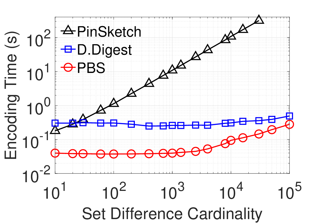
Encoding Time. compares the encoding time of PBS against those of PinSketch and D.Digest. clearly shows that the former is much lower than the latter under all different values of .
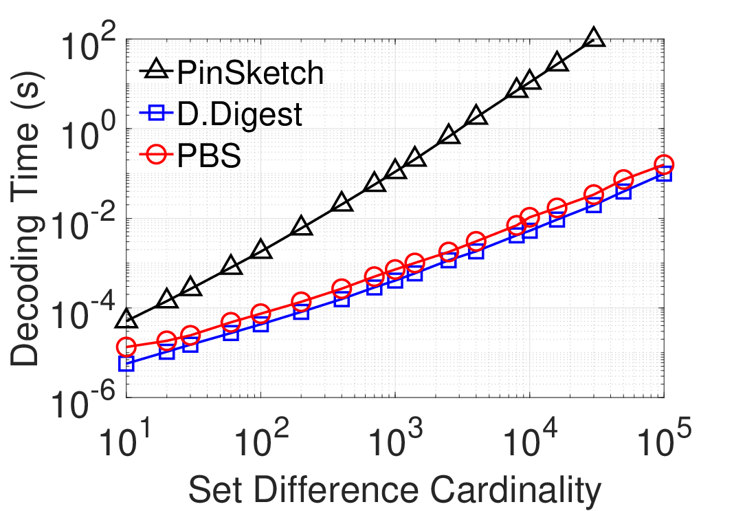
Decoding Time. compares the decoding time of PBS against those of PinSketch and D.Digest. As shown in , the decoding time of PinSketch is much higher than those of D.Digest and PBS when is large (say ). For example, when , the decoding time of PinSketch is roughly three orders of magnitude higher than those of D.Digest and PBS. also shows clearly that D.Digest is the best, whose decoding time is to times shorter than that of PBS.
However, as discussed earlier, the encoding time of D.Digest is much (up to one order of magnitude) longer than that of PBS, and encoding time (of PBS and D.Digest) is usually much longer than the corresponding decoding time. Thus, PBS has the lowest overall computational overhead.
8.2 PBS vs. Graphene
In this section, we compare PBS against Graphene. Recall that in our experimental setting, we have and need to let Alice learn , which was shown in [32] to be the best-case scenario for Graphene in terms of communication overhead and decoding time. Hence we have treated Graphene more than fairly here. Since the parameters in the source code provided by the authors of [32] are already optimized for achieving a target success rate of 239/240, we tune PBS to match this success rate: As shown in , the success rates of both PBS and Graphene are higher than 239/240.
Communication Overhead. compares the communication overhead of PBS against that of Graphene. It shows that, even in this best-case scenario for Graphene, PBS has much lower (roughly 1.2 to 7.4 times less) communication overhead than Graphene under all different values of except when gets very close to . The reason behind this exception was explained earlier (in ): When is sufficiently large with respect to ( in this case), it becomes more communication-efficient overall for Graphene to start using a BF to reduce the size of its IBF. It can be calculated using an optimization formula in [32] that the breakeven point (for using a BF) in this case is some number between and . We can actually see in that the slope of the Graphene curve, which corresponds to the average communication overhead per distinct element, starts to decrease after the breakeven point, resulting in it eventually going under the PBS curve roughly after .
Encoding Time. clearly shows that the encoding time of PBS is to times lower than that of Graphene under all values of .
Decoding Time. compares the decoding time of PBS against those of Graphene and clearly shows that the former is slightly ( to times) longer than the latter except when is close to where the former is up to times longer.
8.3 PBS vs. PinSketch with Partition
Arguably, the same algorithmic trick (i.e., hash-partition and each into groups) can be applied also to PinSketch [13] for reducing its BCH decoding time from to . Doing so however makes the communication overhead of PinSketch higher than that of PBS for the following reason. As explained in , we need to leave a safety margin in setting the BCH error-correction capacity , in the sense that needs to be “comfortably” larger than , the average number of “bit errors” per group. Hence for each group pair, the average additional communication overhead (incurred for transmitting a longer BCH codeword) of leaving this safety margin is in PBS and is in PinSketch. However, as explained in , is typically to times smaller than . Hence PinSketch pays to times more for leaving the safety margin, resulting in a higher overall communication overhead, as we elaborate next.
Now we compare the performance of PBS against that of PinSketch with hash partition, which we refer to as PinSKetch/WP. For PinSketch/WP, we use the same and values as in PBS (there is no parameter in PinSketch/WP since it does not use a parity bitmap), with a target success probability of =0.99 within =3 rounds, in each experiment instance. The experimental results are reported in . It clearly shows that PBS outperforms PinSketch/WP in both communication overhead and computational overhead (the sum of the encoding and the decoding time). Note this outperformance will increase when the hash signature length increases ( bits in ). Hence, PBS would outperform by a wider margin in real-world blockchain applications where is much larger (e.g., bits in Bitcoin [30]), as has been shown in .
9 Conclusion
In this paper, we propose Parity Bitmap Sketch (PBS), a space- and computationally-efficient solution to the set reconciliation problem. We show, through experiments, that PBS strikes a much better tradeoff between communication and computational overheads than all the state-of-the-art solutions. In addition, we derive a novel rigorous analytical framework for PBS, which most existing solutions do not have. Through three applications of this framework, we demonstrate that it enables both the accurate analysis of various performance metrics such as success probability and the tuning of the parameters of PBS for near-optimal performances.
References
- [1] Dropbox smart sync. https://www.dropbox.com/smart-sync. [Online; accessed 23-July-2020].
- [2] Ethereum: A secure decentralised generalised transaction ledger. https://ethereum.org/. [Online; accessed 10-July-2020].
- [3] ProvenDB. https://www.provendb.com/. [Online; accessed 1-June-2020].
- [4] BigchainDB 2.0: The blockchain database. https://www.bigchaindb.com/whitepaper/bigchaindb-whitepaper.pdf, May 2018.
- [5] N. Alon, Y. Matias, and M. Szegedy. The space complexity of approximating the frequency moments. Journal of Computer and System Sciences, 58(1):137–147, 1999.
- [6] B. H. Bloom. Space/time trade-offs in hash coding with allowable errors. Communications of the ACM, 13(7):422–426, July 1970.
- [7] R. C. Bose and D. K. Ray-Chaudhuri. On a class of error correcting binary group codes. Information and Control, 3(1):68–79, 1960.
- [8] A. Z. Broder, M. Charikar, A. M. Frieze, and M. Mitzenmacher. Min-wise independent permutations. Journal of Computer and System Sciences, 60(3):630–659, 2000.
- [9] J. W. Byers, J. Considine, M. Mitzenmacher, and S. Rost. Informed content delivery across adaptive overlay networks. IEEE/ACM Transactions on Networking, 12(5):767–780, Oct. 2004.
- [10] D. Clarke, S. Devadas, M. van Dijk, B. Gassend, and G. E. Suh. Incremental multiset hash functions and their application to memory integrity checking. In Advances in Cryptology - ASIACRYPT 2003, pages 188–207, Berlin, Heidelberg, 2003.
- [11] Y. Collet. xxHash - Extremely fast hash algorithm. https://github.com/Cyan4973/xxHash.
- [12] J. C. Corbett, J. Dean, M. Epstein, A. Fikes, C. Frost, J. J. Furman, S. Ghemawat, A. Gubarev, C. Heiser, P. Hochschild, W. Hsieh, S. Kanthak, E. Kogan, H. Li, A. Lloyd, S. Melnik, D. Mwaura, D. Nagle, S. Quinlan, R. Rao, L. Rolig, Y. Saito, M. Szymaniak, C. Taylor, R. Wang, and D. Woodford. Spanner: Google’s globally distributed database. ACM Transactions on Computer Systems, 31(3):8:1–8:22, Aug. 2013.
- [13] Y. Dodis, R. Ostrovsky, L. Reyzin, and A. Smith. Fuzzy extractors: How to generate strong keys from biometrics and other noisy data. SIAM Journal on Computing, 38(1):97–139, 2008.
- [14] M. El-Hindi, C. Binnig, A. Arasu, D. Kossmann, and R. Ramamurthy. BlockchainDB: A shared database on blockchains. PVLDB, 12(11):1597–1609, July 2019.
- [15] D. Eppstein, M. T. Goodrich, F. Uyeda, and G. Varghese. What’s the difference? efficient set reconciliation without prior context. In Proceedings of the ACM Special Interest Group on Data Communication, pages 218–229, 2011.
- [16] J. Feigenbaum, S. Kannan, M. J. Strauss, and M. Viswanathan. An approximate l1-difference algorithm for massive data streams. SIAM Journal on Computing, 32(1):131–151, Jan. 2003.
- [17] P. Flajolet and G. N. Martin. Probabilistic counting algorithms for data base applications. Journal of Computer and System Sciences, 31(2):182–209, Sept. 1985.
- [18] M. T. Goodrich and M. Mitzenmacher. Invertible bloom lookup tables. arXiv e-prints, arXiv:1101.2245, 2011.
- [19] D. Guo and M. Li. Set reconciliation via counting bloom filters. IEEE Transactions on Knowledge and Data Engineering, 25(10):2367–2380, Oct. 2013.
- [20] N. Hua, A. Lall, B. Li, and J. Xu. A simpler and better design of error estimating coding. In Proceedings of the IEEE International Conference on Computer Communications, pages 235–243, Mar. 2012.
- [21] M. G. Karpovsky, L. B. Levitin, and A. Trachtenberg. Data verification and reconciliation with generalized error-control codes. IEEE Transactions on Information Theory, 49(7):1788–1793, July 2003.
- [22] A. Lakshman and P. Malik. Cassandra: A decentralized structured storage system. ACM SIGOPS Operating Systems Review, 44(2):35–40, Apr. 2010.
- [23] N. Levinson. The wiener (root mean square) error criterion in filter design and prediction. Journal of Mathematics and Physics, 25(1-4):261–278, 1946.
- [24] M. Luby. Tornado codes: Practical erasure codes based on random irregular graphs. In Proceedings of International Workshop on Randomization and Approximation Techniques in Computer Science, pages 171–171, 1998.
- [25] L. Luo, D. Guo, O. Rottenstreich, R. T. Ma, and X. Luo. Set reconciliation with cuckoo filters. In Proceedings of the ACM International Conference on Information and Knowledge Management, pages 2465–2468, 2019.
- [26] R. C. Merkle. A digital signature based on a conventional encryption function. In Proceedings of the Conference on The Theory and Application of Cryptographic Techniques, pages 369–378, Berlin, Heidelberg, 1987.
- [27] Y. Minsky and A. Trachtenberg. Practical set reconciliation. In Proceedings of the Annual Allerton Conference on Communication, Control, and Computing, volume 248, 2002.
- [28] Y. Minsky, A. Trachtenberg, and R. Zippel. Set reconciliation with nearly optimal communication complexity. IEEE Transactions on Information Theory, 49(9):2213–2218, Sept. 2003.
- [29] M. Mitzenmacher and E. Upfal. Probability and computing: Randomization and Probabilistic Techniques in Algorithms and Data Analysis. Cambridge university press, 2017.
- [30] S. Nakamoto. Bitcoin: A peer-to-peer electronic cash system. Technical report, Manubot, 2019. https://bitcoin.org/bitcoin.pdf.
- [31] G. Naumenko, G. Maxwell, P. Wuille, A. Fedorova, and I. Beschastnikh. Erlay: Efficient transaction relay for bitcoin. In Proceedings of the ACM SIGSAC Conference on Computer and Communications Security, pages 817–831, 2019.
- [32] A. P. Ozisik, G. Andresen, B. N. Levine, D. Tapp, G. Bissias, and S. Katkuri. Graphene: Efficient interactive set reconciliation applied to blockchain propagation. In Proceedings of the ACM Special Interest Group on Data Communication, pages 303–317, 2019.
- [33] P. Ruan, G. Chen, T. T. A. Dinh, Q. Lin, D. Loghin, B. C. Ooi, and M. Zhang. Blockchains and distributed databases: a twin study. arXiv e-prints, arXiv:1910.01310, Oct. 2019.
- [34] A. Sharma, F. M. Schuhknecht, D. Agrawal, and J. Dittrich. Blurring the lines between blockchains and database systems: The case of hyperledger fabric. In Proceedings of the ACM SIGMOD International Conference on Management of Data, pages 105–122, 2019.
- [35] M. N. Wegman and J. L. Carter. New classes and applications of hash functions. In Proceedings of the IEEE Annual Symposium on Foundations of Computer Science, pages 175–182, 1979.
- [36] P. Wuille. Minisketch: an optimized library for BCH-based set reconciliation. https://github.com/sipa/minisketch.
- [37] Y. Zhu, Z. Zhang, C. Jin, A. Zhou, and Y. Yan. SEBDB: semantics empowered blockchain database. In Proceedings of the IEEE International Conference on Data Engineering, pages 1820–1831, 2019.
Appendix A Mean and Variance Proof for ToW Estimator
We now prove the claims for the mean and variance of the ToW estimator we made in . Note that, the proof for the mean is almost the same as the proof in [5]; that for the variance is almost the same as that in [20]. We reproduce them with some minor changes (to adapt them to our context) for this paper to be self-contained.
In the following, we first state a well-known fact concerning the four-wise independent hash family that stems from its definition [35].
Fact 1.
If a hash family is four-wide independent, then for any distinct , the hash values are independent and identically distributed random variables, each of which is uniformly distributed in .
We now proceed to prove that the ToW estimator is unbiased, i.e., , as follows.
| (3) | |||||
Equation (3) holds for the following reasons. For any , we have because . Hence, the first and last terms on the LHS of (3) are equal to the corresponding terms on the RHS of (3), respectively. For the second term on the LHS of (3), it is equal to because of and the linearity of expectation. For the same reason, each of the rest two terms on the LHS of (3) is also equal to .
Now, we prove that the claim we made for the variance of , i.e., , as follows.
| (4) | |||||
We note that no terms in the form of (for any distinct ) appear on the RHS of (4), because any such term equals , the expectation of which, as explained earlier, is equal to .
Using the above second moment and the following expression for the variance, of , we have,
| (5) |
Appendix B Other Estimators
Past set reconciliation work mostly uses two other estimators: the min-wise estimator and the Strata estimator [15]. The min-wise estimator is derived from min-wise hashing technique [8] for estimating set Jaccard similarity . The Strata estimator is based on the idea of Flajolet and Martin (FM) sketch [17], originally designed for estimating , the zeroth frequency moment of a data stream. In comparison, the ToW estimator is much more space-efficient according to our experiments under various parameter settings. The results are not shown here in the interest of space.
The sketch, proposed in [16] and designed for estimating the -difference between two functions, can also be used to estimate the set difference cardinality. It has similar space-efficiency as the ToW estimator. However, it is much less computationally-efficient, as it requires a nontrivial amount of computation for constructing random variables that are range-summable – a property that is not needed for our application.
Appendix C Correctness of PBS
In this section, we formally prove the correctness of PBS, more precisely PBS-for-large-d. It suffices to prove the correctness of PBS-for-small-d, because the reconciliation of each group pair in PBS-for-large-d is solved by PBS-for-small-d. The following theorem states the correctness of PBS-for-small-d.
Theorem 1.
Assume that the checksum verification step in of produces correct verifications (in every round). If PBS-for-small-d terminates after rounds, then
Proof.
Since PBS-for-small-d terminates after rounds, the checksum verification step ( of ) must have succeeded in the round. Hence we have . Since we assume that the checksum verification step produces correct verifications, we have . Therefore,
∎
Appendix D Preciseness of Markov-Chain Modeling
The Markov-chain model in precisely captures every detail of the set reconciliation process in each group pair except for one event: when a fake distinct element resulting from a type (II) exception is indeed not a distinct element but “luckily” (unluckily for Alice) passes the sub-universe verification check () and gets included in the estimated set difference in the correspoinding round. We choose to leave this event out in the modeling, because to incorporate it would result in a much more complicated Markov chain. To incorporate this event is also not necessary for our modeling to be numerically accurate, because this event happens with a tiny probability of .
In this model, we assume , where is the error-correction capacity of the BCH code. To extend the Markov-chain modeling to the case of (resulting in a BCH decoding failure w.h.p.) is a daunting task, since this group pair is to be partitioned into sub-group-pairs as described in and each sub-group-pair is to be independently reconciled. We also found this task unnecessary: Assuming when in our modeling (always to our disadvantage) results in only a slight underestimation of “good” probabilities, as will be elaborated in .
Appendix E How To Compute
Although the transition probability matrix is in theory an infinite matrix, in this work for all practical purposes (e.g., for computing ), it can be considered a matrix, where is the BCH error-correction capacity. In this section, we describe how to compute the transition probability matrix in detail. To compute is not straightforward for the following reason. Each state with in the Markov chain is a composite state consisting of a large number of atom states. Only the transition probability from state to any atom state (of state ) can be stated as a closed-form expression (more precisely, a multinomial formula) and computed straightforwardly. The value of is the total of all the transition probabilities from state to each of the atom states of state . Since the number of atom states grows exponentially with , it is complicated (as it is necessary to enumerate all atom states), error-prone, and computationally expensive to compute this way when is large (say ), as we will elaborate next.
Each atom state of state is, in combinatorics terms, a permutation of a combination of , which here corresponds to how these balls are distributed in the bins (by the hash function). For a simple example, when and , the vector is such an atom state, which corresponds to these bins (in a predefined order such as the natural order) having and “bad” balls in them respectively. Clearly, the number of such atom states (vectors) grows exponentially with . For instance, when , the number of distinct atom state vectors is , , , , respectively. Although the computation of can be simplified by the fact that two atom states have the same transition probability (i.e., belong to the same equivalence class) from the same state if one’s state vector (e.g., in the example above) is a permutation of the other’s (e.g., ), grouping such a large number of atom states into equivalence classes and computing the total transitioning probability of each is a complicated and error-prone process.
Our solution is to decompose each composite state into a much small number of coarse-grained sub-states, each of which may still contain a large number of atom states. Although the transition probability from a state to any sub-state of is still a summation formula and hence hard to compute in the “mundane” way as explained above, we discover a recurrence relation among these transition probabilities that makes them easily computable using dynamic programming.
We now define these sub-states and describe the recurrence relation among the resulting transition probabilities. Each state (“bad” balls) is decomposed into sub-states that we denote as , , , , respectively. Each sub-state , , corresponds to the set of scenarios in which the “bad” balls end up occupying exactly “bad” bins (those containing more than one “bad” balls as defined earlier in ). Let denotes the event that throwing balls results in the sub-state . Let denote the probability of this event . Clearly, we have for .
To obtain , it suffices to compute the probabilities of for . To do so, we derive a recurrence relation for these probability values by rendering the process of throwing balls “in slow motion” in the following sense: We throw them one at a time. Now consider what events happen before and after the ball is thrown. Suppose the event happens after the ball is thrown. There are only three possible events before the ball is thrown that can lead to the event . Here we explain only the first event in detail, as explanations for the other two are similar. The event leads to the event if and only if the ball lands in a previously “good” bin so that the “good” ball already in the bin and the ball turn into two “bad” balls. The latter happens with probability , since out of bins are “good” at sub-state . The other two events are and , and they lead to the event with probability and respectively. Summarizing these three cases, we can express , the probability of the event , as the weighted sum of the probabilities of these three events as follows:
Exploiting these recurrence relations (for ), we can compute the values of all the terms in time via dynamic programming, for which the probability formulae of the three types of base cases are:
Appendix F Success probability analysis
As explained earlier in , in PBS-for-large-, the sets and each needs to be hash-partitioned into groups. Let be the numbers of distinct elements contained in these group pairs respectively. It is not hard to check that random variables are identically distributed with distribution (since each of the distinct elements between and is uniformly at random hash-partitioned into one of the groups). Let , , be the number of rounds it takes for the reconciliation of group pair to be successfully completed. Then by definition, we have . Since have the same distribution , it suffices to derive , the success probability for group pair , as the success probability for any other group pair is identical. Replacing by in Formula , we obtain .
As discussed in , to our disadvantage, we assume when (the BCH error-correction capacity). However, this assumption results in only a slight underestimation of the success probability for the following reason. The Binomial term , the “coefficient” of , is very small when since and is typically set to between to times of . For notational succinctness, we denote this slightly underestimated success probability as in the sequel. Clearly, the success probability for any other group pair is also bounded by .
By definition, we have . However, we cannot state rigorously that the overall (for all group pairs) success probability is lower bounded by , because each is a function of the random variable , and the random variables , , …, are not mutually independent as their sum is . However, in this special case of identically binomially distributed random variables with a fixed sum, we can prove, using Corollary 5.11 in [29], a rigorous and only slightly weaker lower bound of for : It only doubles the failure probability in the unrigorous lower bound (written as ) to in the rigorous bound.
Appendix G Analysis on “Piecewise Reconciliability”
Again we focus our attention on the first group pair that have (distributed as as explained earlier) distinct elements between them. Let , , be the number of distinct elements among those that are reconciled in the round. Clearly, our goal is to compute , , , …, and so on. To do so, it suffices to compute the unconditional expectations for . They in turn can be derived from the following conditional expectations on the LHS of Equation . Equation holds because both sides calculate the expected number of distinct elements that are reconciled within rounds, conditioned upon the event .
| (12) |


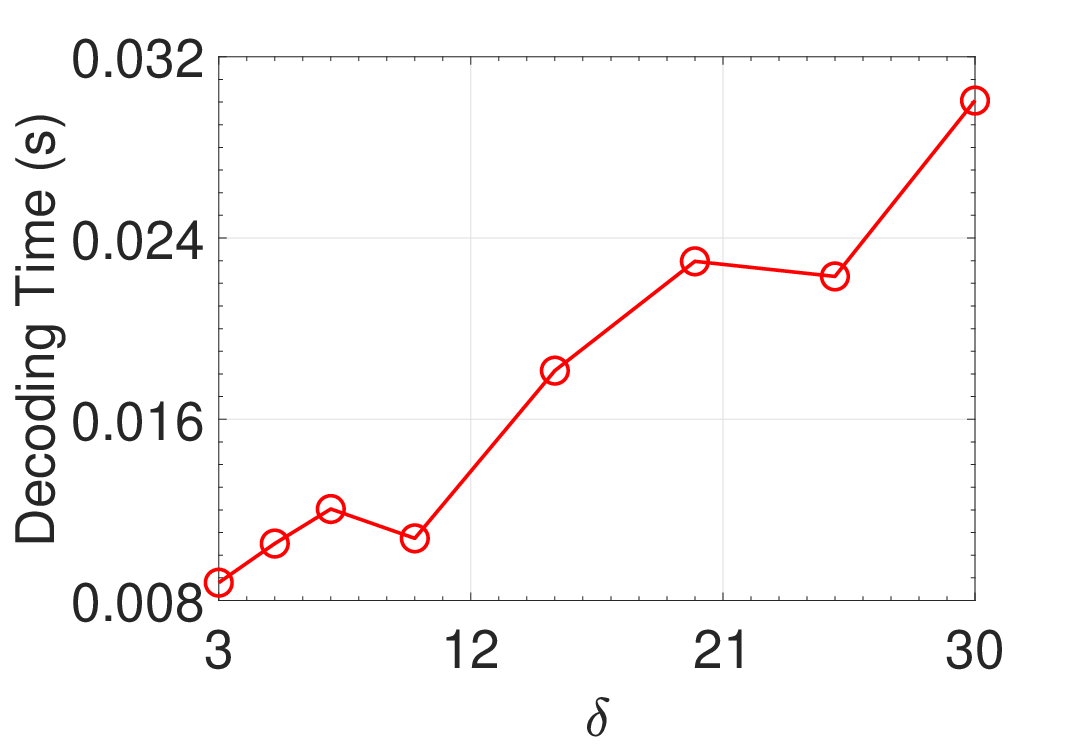
Appendix H An Example for Parameter Optimization
| 8 | 0 | 25.5% | 32.7% | 34.3% | 34.9% | 35.0% |
| 9 | 52.1% | 78.0% | 84.2% | 85.7% | 86.1% | 86.2% |
| 10 | 75.1% | 92.7% | 96.5% | 97.4% | 97.6% | 97.7% |
| 11 | 85.9% | 96.9% | 99.1% | 99.5% | 99.6% | 99.6% |
| 12 | 91.3% | 98.5% | 99.7% | 99.9% | 99.9% | 99.9% |
| 13 | 93.9% | 99.1% | 99.8% | 99.9% | 99.9% | 99.9% |
| 14 | 95.1% | 99.4% | 99.9% | 99.9% | 99.9% | 99.9% |
| 15 | 95.6% | 99.5% | 99.9% | 99.9% | 99.9% | 99.9% |
| 16 | 95.7% | 99.6% | 99.9% | 99.9% | 99.9% | 99.9% |
| 17 | 95.8% | 99.6% | 99.9% | 99.9% | 99.9% | 99.9% |
In this section, we illustrate our parameter optimization procedure described in with an example. Suppose we have distinct elements, (so that groups), rounds, and target success probability . For each value combination in we compute the corresponding lower bound () value. The lower bound values corresponding to these value combinations are shown . In , each cell in which the corresponding lower bound value is no smaller than the target success probability is highlighted. Among the highlighted cells, the cell further darkened results in the smallest objective function value and hence its “coordinates” are the optimal parameter setting in this instance. Using pre-computation, the success probability value in each cell can be computed in time, so this optimization procedure is very efficient computationally.
Appendix I Use of BCH in Communication
In this section, we describe the standard BCH encoding for its usual application of communication over a noisy channel and explain how it differs from the BCH encoding in PBS. In the standard BCH encoding, a coded message, which is the uncoded message concatenated with the codeword, is bits long in total. For the codeword to correct up to bit errors, that may occur to both the uncoded message part and the codeword part during the transmission of the coded message over the noisy channel, it needs to be bits long, resulting in a “leftover” of at most bits for the uncoded message.
In PBS, the codeword is also bits long, but the uncoded message (which is not transmitted at all) can be bits (instead of bits) long. The uncoded message is allowed to be longer here because, unlike in the usual application of communication over a noisy channel where bit errors can happen also to the codeword, in PBS no bit error will happen to the codeword during its transmission.
Appendix J More Experimental Results
J.1 Number of Rounds Required by PBS
| 1 | 2 | 3 | |
| 0.804 | 0.188 | 0.008 | |
| 0.217 | 0.760 | 0.023 | |
| 0 | 0.957 | 0.043 | |
| 0 | 0.907 | 0.093 | |
| 0 | 0.818 | 0.182 |

In this section, we investigate the empirical number of rounds required by PBS to correctly reconcile all distinct elements. The parameter settings are exactly the same as those we used in . The only difference is that we let PBS run as many as rounds it requires instead of only allowing it running at most rounds.
presents the empirical distributions of the number of rounds required by PBS to correctly reconcile all distinct elements, with the set difference cardinality =. It is easy to verify that the average numbers of rounds are for = respectively. Furthermore, in every experiment the reconciliation process took no more than 3 rounds to complete. Hence the probability values in every row of add up to (probability) .
J.2 PBS Performances When Varying
In this section, we investigate the performance of PBS under different values of , where is the average number of distinct elements per group pair. We have considered a constant throughout this paper, but in this section only, we consider it a tunable parameter. In our experiments, we vary between and . Like in , for each value, we set the values of the other parameters of PBS in such a way that it guarantees to correctly reconcile all distinct elements in no more than rounds with a probability of at least . We have experimented with different values of (the set difference cardinality). Here we only present the results for =, as other values of lead to similar conclusions.
The experimental results, shown in , confirm our earlier claim that can serve as a knob to control the tradeoff between communication and computational overheads in PBS. shows that the communication overhead of PBS generally decreases as grows, whereas and show that both the encoding time and the decoding time of PBS increase as grows.
J.3 PBS vs. PinSketch with Partition
In this section, we compare again the performance of PBS and PinSketch/WP when the hash signature length . As the implementations of all the evaluated algorithms do not support signature length higher than bits (one of them only supports 32 bits), the results here are obtained through simulations with a -bit universe. Thus, we only present the results for communication overheads. The results are shown in .
(comparing with ) clearly shows that the outperformance of PBS over PinSketch/WP is more significant (than that in ).