Estimation of local treatment effects under the binary instrumental variable model
1Linbo Wang, 2Yuexia Zhang, 3Thomas S. Richardson, 4James M. Robins
1,2University of Toronto, 3University of Washington, 4Harvard T.H. Chan School of Public Health
Keywords: Causal inference; Model compatibility; Variation independence; Semiparametric efficiency.
Abstract
Instrumental variables are widely used to deal with unmeasured confounding in observational studies and imperfect randomized controlled trials. In these studies, researchers often target the so-called local average treatment effect as it is identifiable under mild conditions. In this paper, we consider estimation of the local average treatment effect under the binary instrumental variable model. We discuss the challenges for causal estimation with a binary outcome, and show that surprisingly, it can be more difficult than the case with a continuous outcome. We propose novel modeling and estimating procedures that improve upon existing proposals in terms of model congeniality, interpretability, robustness or efficiency. Our approach is illustrated via simulation studies and a real data analysis.
Abstract
In the Supplementary Material we provide proofs of theorems and claims in the main paper. We also provide additional details for the simulations and data application.
1 Introduction
Unmeasured confounding is a common threat to draw valid causal inference in practice. It can occur in observational studies as well as imperfect randomized controlled studies where participants may not comply with the assigned treatment. Instrumental variable methods which seek to address this, are widely used in economics, biostatistics and epidemiology to estimate causal effects when unmeasured confounders may be present. Intuitively, an instrumental variable is a pre-treatment covariate that is associated with the outcome only through its effect on the treatment. In practice, the condition above is often reasonable only after controlling for a set of baseline covariates.
Traditionally, instrumental variable methods have aimed to estimate average treatment effects (Wright and Wright, 1928; Goldberger, 1972). Identification of the average treatment effects, however, relies on untestable homogeneity assumptions involving unmeasured confounders (Hernán and Robins, 2006; Wang and Tchetgen Tchetgen, 2018, e.g.). An alternative proposed by Imbens and Angrist, 1994 and Angrist et al., 1996 is to estimate the so-called local average treatment effects as they can be non-parametrically identified under a certain monotonicity assumption. In the non-compliance setting, the local average treatment effects may be of interest in practice since if the local effect indicates that treatment is advantageous then this can be used as an argument for increasing the incentives for taking the treatment.
The estimation problem of local average treatment effects has been studied extensively for continuous outcomes (Abadie et al., 2002; Abadie, 2003; Tan, 2006; Okui et al., 2012; Ogburn et al., 2015, e.g.). However, as explained in detail in Section 2, direct application of these methods to binary outcomes is often inappropriate. Furthermore, with the exception of Ogburn et al., 2015 and Abadie, 2003, most existing methods only focus on the additive local average treatment effect but not the multiplicative local average treatment effect; the latter is of common interest with binary outcomes as it measures the causal effect on the relative risk scale. In related work, the Wald-type estimator of Didelez et al., 2010 can be shown to be approximately equal to the multiplicative local average treatment effect under a monotonicity assumption (Clarke and Windmeijer, 2012).
In this paper, we propose novel estimating procedures for both the additive and multiplicative local average treatment effects with a binary outcome that (a) ensure the posited models are variation independent and hence congenial with each other (Meng, 1994); (b) ensure the resulting estimates lie in the natural non-trivial parameter space; (c) directly parameterize the local average treatment effect curves to improve interpretability and reduce the risk of model mis-specification (Ogburn et al., 2015); (d) allow for efficient and truly doubly robust estimation of the causal parameter of interest. To the best of our knowledge, for the additive local average treatment effect, our procedure is the first one that achieves (d); for the multiplicative local average treatment effect, our procedure is the first one that achieves (a),(c) or (d); see also Remark 3.
2 Framework, notation and existing estimators
Consider the problem of causal effect estimation with a binary exposure indicator and a binary outcome . Suppose the effect of on is subject to confounding by observed variables as well as unobserved variables . Following the potential outcome framework, we assume , the potential exposure if the instrumental variable would take value , to be well-defined. Similarly, we assume , the outcome that would have been observed if a unit were exposed to and the instrument had taken value , to be well-defined. We assume we also observe a binary instrumental variable that satisfies the following assumptions (Angrist et al., 1996):
- A1
Exclusion restriction: for all and , almost surely;
- A2
Independence: ;
- A3
Instrumental variable relevance: almost surely;
- A4
Positivity: there exists such that almost surely;
- A5
Monotonicity: almost surely.
Notably implicit in the notation is that the instrument is causal so that A3 implies that has a non-zero causal effect on . Figure 1 gives a simple illustration of the conditional instrumental variable model; see Figure S2 in the Supplementary Material for another example.
Under the principal stratum framework (Frangakis and Rubin, 2002), the population can be divided into four strata based on values of as in Table 1. We use to denote principal stratum defined by values of .
| Principal stratum | Abbreviation | ||
|---|---|---|---|
| 1 | 1 | Always taker | AT |
| 1 | 0 | Complier | CO |
| 0 | 1 | Defier | DE |
| 0 | 0 | Never taker | NT |
We are interested in estimating the conditional treatment effects in the complier stratum on the additive and multiplicative scales defined as
For to be well-defined, we also assume that almost surely. By definition, the parameter space of and are constrained: while
Abadie, 2002 shows that under assumptions A1-A5, the local average treatment effects are identifiable as
| (1) | ||||
| (2) |
Given (1), it might be tempting to estimate and hence with a plug-in estimator by first estimating the four curves and separately, as proposed by Frölich, 2007. However, even though one may choose suitable models so that estimates for the four curves above lie in the unit interval, there is no guarantee that the plug-in estimator is between -1 and 1. The same problem arises when applying Tan, 2006’s approach that imposes parametric models on the conditional means and . Similar problems arise with plug-in estimators for .
To avoid these problems, Abadie, 2003 specifies a parametric model, such as the logistic model, for the so-called local average response function The model parameters are then estimated by a weighted estimating equation. The parameters of logistic models, however, do not directly encode the dependence of local average treatment effects on baseline covariates, so they do not offer direct insights into which baseline variables modify the local average treatment effects. Moreover, the validity of their approach hinges on correct specification of the instrumental density . Instead, Okui et al., 2012 and Ogburn et al., 2015 propose doubly robust estimators based on direct parameterization of the target functional . Given a correct model , their estimators are consistent and asymptotically normal for the parameter of interest if either the instrumental density model or another nuisance model is correctly specified. However, the nuisance model is variation dependent of the target model . In this case, the double robustness property of Okui et al., 2012 and Ogburn et al., 2015’s estimators is not practically meaningful since with continuous covariates, often it is not possible for and to be correct simultaneously. Similar discussions apply to the target functional
In related work, Wang and Tchetgen Tchetgen, 2018 studied the problem of estimating a closely related functional, , which may be interpreted as the average treatment effect under a certain set of identification assumptions. As an intermediate step, Wang and Tchetgen Tchetgen, 2018 propose alternative nuisance models that are variation independent of including a model for . The key observation made by these authors is that as long as the models for and both lie in their parameter space, which is for and for , then
also lies in its parameter space Following this, they derive a maximum likelihood estimator (Wang and Tchetgen Tchetgen, 2018, §4.1) and a truly doubly robust estimator for (Wang and Tchetgen Tchetgen, 2018, equation (14)). These approaches, however, cannot be adapted to estimate or the multiplicative local average treatment effect. Furthermore, as we explain later in Remark 2, even for the additive local average treatment effect, in general their doubly robust estimator fails to achieve the semiparametric efficiency bound.
3 A novel parameterization
In this section we describe a novel parameterization of the observed data likelihood involving or Specifically, our goal is to find nuisance models so that (I) they are variation independent of each other; (II) they are variation independent of and ; (III) there exists a bijection between the observed data likelihood on and the combination of target and nuisance models. Note the remaining parts of the likelihood on do not show up in the identification formula (1) or (2). Thus they contain no information about the parameters of interest and need not be modeled.
Let For any , the parameter space of the observed data likelihood on is a six-dimensional space in (Richardson et al., 2011):
| (3) |
Parameterization of is a difficult problem since as shown by (3), the likelihood components are not variation independent of each other.
To make progress, instead of modeling the observed likelihood components directly, we seek to model components of the potential outcome likelihood conditional on . Specifically, we will consider and and . The remaining parts of the potential outcome likelihood, such as are not modeled as they are not related to the observed data likelihood, and hence contain no information for the parameters of interest. These components, however, are still variation dependent since
| (4) |
Moreover, they do not contain our target function or which we denote as .
Theorem 1 presents an alternative parameterization that satisfies goals (I)–(III). To avoid the constraint (4), we follow Wang et al., 2017c to re-parameterize . To re-parameterize and so that the new parameterization includes , we follow Richardson et al., 2017 to model an odds product function in the complier stratum. The proof of Theorem 1 is left to the Supplementary Material.
Theorem 1
Let denote the 6-dimensional models consisting of the target model and models on the following nuisance functions:
where denotes odds product in the complier stratum.
Under assumptions A1 - A5, for any realization of , the map given by
| (5) |
is well-defined and is a smooth bijection from to , where if and if Furthermore, the models in are variation independent of each other.
Suppose models for are all specified up to a finite dimensional parameter, then these parameters, and in particular the local average treatment effects may be estimated directly via unconstrained maximum likelihood based on the diffeomorphism (5). Likelihood-based confidence intervals can then be obtained in standard fashion.
Remark 1
Since the constituent models, , are variation independent, the modeler is free to pick any function of with the given range. For example, to mitigate model mis-specification, one may assume flexible machine learning models on these functions of . In this case, one can similarly fit these flexible models based on the implied models on the likelihood
4 Doubly Robust Estimation
In this section we apply our parameterization in Theorem 1 to construct truly doubly robust estimators that are asymptotically linear for estimating the local average treatment effects if either the nuisance models or the instrumental density model is correct, given that the causal model is correctly specified. These estimators are called truly doubly robust because, as shown in Theorem 1, the nuisance models and causal model are variation independent and hence congenial to each other.
Let and be the maximum likelihood estimators of . Also let
We have the following theorem.
Theorem 2
Let solve the following estimating equation:
| (6) |
where
with
and
denotes the empirical mean operator and is an arbitrary measurable function of . Then under a correct model for and regularity conditions, is consistent and asymptotically normally distributed provided that at least one of the models for or is correctly specified. The optimal choice of that minimizes the asymptotic variance of is given in the Supplementary Material.
Theorem 2 is a special case of the doubly robust g-estimation theory developed by Ogburn et al., 2015. For completeness, we provide the proof in the Supplementary Material. One can also easily verify that the arguments in the square roots in are always non-negative, provided that the estimates of and stay within their respective domain. Statistical inference may be based on standard M-estimation theory. Alternatively, in the simulations and real data analysis, we use nonparametric bootstrap.
Remark 2
When Wang and Tchetgen Tchetgen, 2018’s approach parameterizes the marginal distributions and , whereas our approach parameterizes the joint distribution On the other hand, in addition to the marginal distributions, the optimal choice of also depends on . Hence it can be calculated based on our parameterization but not Wang and Tchetgen Tchetgen, 2018’s.
Remark 3
Prompted by the comment of a referee, we notice that if then . Hence a simple way to estimate based on (6) is to first obtain estimates of and and then plug these estimates into (6) to estimate . Moreover, in the Supplementary Material, we show that and are variation independent in the interior of their domains; a similar phenomenon was previously observed by Wang et al., 2017a. Similarly, if then Hence a simple way to estimate based on (6) is to first obtain estimates of and , and then plug these estimates into (6) to estimate . and are also variation independent in the interior of their domains. Consequently, since all the nuisance models can, logically, be correctly specified, these simple estimators are truly doubly robust assuming that the true parameter values are away from the boundary. However, similar to the estimator of Wang and Tchetgen Tchetgen, 2018, they cannot be used to estimate the optimal . Furthermore, these simple parameterizations do not lead to likelihood-based inference.
5 Simulation studies
In this section, we evaluate the finite sample performance of various estimators discussed in this paper. We generate data from the following models:
where the covariates include an intercept and a random variable generated from ; , , , and . Under this setting, the strength of instrumental variable, defined as , is . The sample size is .
We also consider scenarios in which the nuisance models are mis-specified. In these scenarios, the analyst is given covariates including an intercept and an irrelevant covariate generated from an independent , and covariates including
Instead of formulating a model conditioning on , the analyst fits the model and/or , , . The analyst still uses the correct functional form in these models. The target model is always correctly specified. Figure S1 in the Supplementary Material visualizes the degree of model mis-specification by showing the data points generated under the true models and mis-specified models from one randomly selected Monte Carlo run.
We consider the performance of following estimators:
- mle:
the proposed maximum likelihood estimator;
- drw:
the proposed doubly robust estimator with the optimal weighting function;
- dru:
the proposed doubly robust estimator with the identity weighting function;
- reg.ogburn:
Ogburn et al., 2015’s outcome regression estimator;
- drw.ogburn:
Ogburn et al., 2015’s doubly robust estimator with the optimal weighting function;
- dru.ogburn:
Ogburn et al., 2015’s doubly robust estimator with the identity weighting function;
- mle.wang:
Wang and Tchetgen Tchetgen, 2018’s maximum likelihood estimator;
- dru.wang:
Wang and Tchetgen Tchetgen, 2018’s doubly robust estimator with the identity weighting function;
- dru.simple:
The doubly robust estimator described in Remark 3;
- ls.abadie:
Abadie, 2003’s least squares estimator;
- mle.crude:
Richardson et al., 2017’s maximum likelihood estimator of the crude association on the additive/multiplicative scale.
For models other than the proposed ones, we provide details of model specifications in the Supplementary Material.
Throughout our simulations, we assume the model of interest is always corrected specified. We consider the following four scenarios for the nuisance models:
- bth:
is used in all nuisance models;
- psc:
is used in the instrumental density model, but is used in other nuisance models;
- opc:
is used in the instrumental density model, but is used in other nuisance models;
- bad:
is used in the instrumental density model, and is used in other nuisance models.
As Abadie, 2003’s method does not directly specify a model for , we consider the following two scenarios for their method:
- bth:
is used in all models;
- bad:
is used in the instrumental density model, but is used in the model for .
The implied model for remains correct in either of these two scenarios.
Table 2 presents selected results of the bias and the Monte-Carlo standard error for various estimators based on Monte-Carlo runs. In Section 5.3 of the Supplementary Material, we present the complete set of results in Table S2, and bias as a percentage of the estimator’s standard deviation in Table S3. The estimator mle.crude has large bias, indicating that the effect of unmeasured confounding is non-negligible. As expected, the proposed estimators have small bias relative to standard error in all scenarios except for mle.bad and drw.bad. As expected, when all nuisance models are correctly specified, the proposed maximum likelihood estimator has smaller or comparable standard error to the optimally-weighted doubly robust estimator drw.bth. The performance of dru.ogburn.bth, dru.wang.bth and dru.simple.bth are all similar to that of dru.bth; all these four methods are less efficient than drw.bth. This suggests that under our simulation settings, the optimal weighting function leads to important efficiency gain. Although drw.ogburn.bth is constructed based on the same optimally weighted estimating equation as drw.bth, mis-specification of variation dependent models leads to a biased estimate of the optimal weight function. As a result, in some cases, it is even less efficient than dru.ogburn.bth.
| Bias (SE ) | ||||
|---|---|---|---|---|
| mle.bth | 0.28(0.35) | -3.5(0.78) | -0.092(0.71) | -3.0(1.2) |
| mle.bad | -20(0.42) | -15(0.80) | -48(1.2) | -18(2.1) |
| drw.bth | 0.55(0.36) | -4.1(0.82) | 0.54(0.77) | -5.6(1.5) |
| drw.psc | 0.060(0.38) | -5.9(1.0) | -0.38(1.2) | -12(2.7) |
| drw.opc | 0.55(0.36) | -3.9(0.79) | 0.49(0.75) | -5.3(1.4) |
| drw.bad | -10(0.40) | -9.6(1.1) | -28(1.4) | 25(3.3) |
| dru.bth | 1.3(0.44) | -5.8(1.0) | 1.8(0.84) | -8.1(1.7) |
| reg.ogburn.bth | -5.7(1.6) | -2.9(3.1) | 7.8(2.0) | -1.1(2.2) |
| reg.ogburn.bad | -9.0(0.25) | 100(0.23) | 140(5.6) | 93(3.6) |
| drw.ogburn.bth | 0.10(0.46) | -4.2(0.99) | 3.2(1.4) | -13(2.5) |
| dru.ogburn.bth | 1.3(0.45) | -5.8(1.1) | 1.9(0.85) | -8.2(1.7) |
| dru.wang.bth | 1.3(0.45) | -5.8(1.0) | ||
| dru.simple.bth | 1.3(0.45) | -5.8(1.0) | 1.8(0.84) | -8.0(1.7) |
| dru.simple.psc | 1.2(0.44) | -6.2(1.0) | 1.9(0.84) | -8.8(1.7) |
| dru.simple.opc | 4.5(0.49) | -17(1.2) | -0.15(0.68) | 11(1.2) |
| dru.simple.bad | -16(0.48) | -17(1.3) | -34(0.70) | 18(1.5) |
| ls.abadie.bth | -0.19(0.37) | -4.1(0.93) | 0.42(0.79) | -11(1.6) |
| ls.abadie.bad | -23(0.88) | 22(1.2) | -32(1.9) | 7.7(3.6) |
| mle.crude | -2.8(0.10) | 60(0.19) | 0.36(0.25) | 51(0.42) |
Table 3 reports selected coverage probabilities of 95% confidence intervals obtained from quantile bootstrap based on 500 bootstrap samples, with the complete set of results presented in Table S4 in the Supplementary Material. The proposed estimators has coverage close to the nominal level except that for mle.bad and drw.bad. Inference results produced by reg.ogburn.bth and drw.ogburn.bth tend to be overly conservative, possibly due to mis-specification of variation dependent models.
| Coverage probability | ||||
|---|---|---|---|---|
| mle.bth | 95.6 | 95.8 | 95.4 | 96.4 |
| mle.bad | 65.4 | 91.0 | 46.3 | 94.6 |
| drw.bth | 94.7 | 95.2 | 96.9 | 95.9 |
| drw.psc | 95.4 | 95.5 | 97.6 | 97.4 |
| drw.opc | 95.0 | 95.6 | 96.1 | 96.1 |
| drw.bad | 87.0 | 95.3 | 91.8 | 96.8 |
| dru.bth | 94.5 | 94.6 | 96.3 | 96.9 |
| reg.ogburn.bth | 98.0 | 99.9 | 99.6 | 100.0 |
| reg.ogburn.bad | 75.6 | 0.1 | 99.9 | 86.1 |
| drw.ogburn.bth | 97.0 | 98.1 | 98.5 | 98.4 |
| dru.ogburn.bth | 94.5 | 95.0 | 96.2 | 97.2 |
| dru.wang.bth | 94.4 | 94.7 | ||
| dru.simple.bth | 94.3 | 94.8 | 96.1 | 96.5 |
| dru.simple.psc | 94.7 | 94.6 | 96.1 | 96.8 |
| dru.simple.opc | 93.6 | 92.6 | 96.2 | 94.9 |
| dru.simple.bad | 76.3 | 94.4 | 69.3 | 93.8 |
| ls.abadie.bth | 94.8 | 95.5 | 96.4 | 95.6 |
| ls.abadie.bad | 87.3 | 94.5 | 93.1 | 95.7 |
| mle.crude | 84.3 | 0.0 | 94.0 | 6.3 |
6 Application to 401(k) data
We apply the proposed procedures to evaluate the effect of 401(k) retirement plan on savings, which has become the most popular employer-sponsored retirement plan in the United States. Economists have long been interested in whether 401(k) contributions represent additional savings or simply replace other retirement plans, such as Individual Retirement Accounts. To account for unobserved confounders such as the underlying preference for savings, Abadie, 2003 chooses 401(k) eligibility as an instrument. Since eligibility is determined by employers, individual preferences for savings may play a minor role in the determination of eligibility after controlling for observed covariates including family income, age, marital status and family size. Furthermore, it is plausible that 401(k) eligibility has an impact on participation in Individual Retirement Accounts only through participation in 401(k) plans. The monotonicity and instrumental variable relevance assumptions hold trivially as only eligible individuals may choose to participate in 401(k) plans.
In our analysis, we use the data set prepared for Abadie, 2003, which contains 9275 individuals from the Survey of Income and Program Participation of 1991. The study participants were between 25 and 64 years old, had an annual income between $10,000 and $200,000 and a family size ranging from 1 to 13; 62.9% of them were married. The assumptions A1, A2 of the instrumental variable model imply restrictions on the observed data law (Pearl, 1995). Wang et al., 2017b show that these restrictions may be tested by applying a modified Gail-Simon test for interaction after re-coding the data. Applying this test to the data considered by Abadie, 2003 confirms that they are compatible with A1 and A2 at level 0.05. The Gail-Simon test was performed conditional on the discrete covariates: family income $20,000, $20,000-30,000, $30,000-40,000, $40,000-50,000, $50,000-75,000 and above $75,000; age 29 years old or younger, 30-35 years old, 36-44 years old, 45-54 years old, and 55 years old or older; a marriage indicator.
In the following, we use Abadie, 2003’s instrumental variable model to estimate the multiplicative local average treatment effect of 401(k) participation on the probability of holding an Individual Retirement Accounts. Figure S2 in the Supplementary Material gives a graphical representation of the instrumental variable model assumed in our analysis. Throughout we make the following assumption on the local average treatment effect:
| (7) |
where the covariates include an intercept, family income, family income squared, age, marital status and family size. Since there are no defiers or always takers, the multiplicative local average treatment effect can also be interpreted as the multiplicative treatment effect of 401(k) participation among those who actually participated in 401(k) plans. We apply the following estimation methods previously evaluated in the simulations: mle, drw, drw.ogburn, dru.ogburn, dru.simple, ls.abadie and mle.crude. Since only eligible individuals may participate in 401(k) plans, one can show that and , where . Similar to the proof of Theorem 1, one can show that in this situation, the models of , can be determined by the models of and . We provide details of model specifications in Section 5.5 of the Supplementary Material. The confidence intervals are obtained based on 500 bootstrap samples.
Figure 2 compares coefficient estimates for model (7). For example, results by mle suggests that with each additional family member, the multiplicative effect of 401(k) participation on holding an IRA account increases by (95% CI = [-0.3%, 15.1%]). Results for drw.ogburn are not plotted as its variance is huge compared to the other estimators. This suggests that the model for and/or the model for are probably mis-specified. For the rest, the 95% confidence intervals obtained using drw are narrower than those obtained using dru.ogburn and dru.simple. This suggests that adopting the optimal weighting function is useful for reducing the variability of effect estimates. None of the covariates considered here is a significant modifier for the crowding out effect of the 401(k) plan at level 0.05.
We also examine representative subgroups for married and unmarried individuals and present the results in Figure 3. The typical married subjects in this data set, defined by the median of individual covariates, were 40 years old, had an annual income of $40530 and a family of size of 4. Correspondingly, the typical unmarried subjects in this data set were 39 years old, had an annual income of $23718 and no other family members. Analysis results from mle suggest that for a typical married subject, participation in the 401(k) program increases the likelihood of holding an IRA account by 14.7% (95% CI = [-1.2%, 33.3%]). In comparison, participation in the 401(k) program has virtually no effect on holding an IRA account for a typical unmarried subject. In either case, there is no evidence for the crowding out effect of 401(k) participation. Comparing the results of mle.crude with mle and drw, Figure 3 shows that the instrumental variable methods attenuate the estimated effect of 401(k) participation on the probability of holding an Individual Retirement Account. These findings are consistent with the observations by Abadie, 2003.
Acknowledgments
The authors thank Elizabeth Ogburn for helpful conversations, and the referees and the associate editor for their insightful comments. This research was supported by grants from Natural Sciences and Engineering Research Council of Canada, U.S. National Institutes of Health and Office of Naval Research.
References
- Abadie, (2002) Abadie, A. (2002). Bootstrap tests for distributional treatment effects in instrumental variable models. Journal of the American Statistical Association, 97(457):284–292.
- Abadie, (2003) Abadie, A. (2003). Semiparametric instrumental variable estimation of treatment response models. Journal of Econometrics, 113(2):231–263.
- Abadie et al., (2002) Abadie, A., Angrist, J. D., and Imbens, G. W. (2002). Instrumental variables estimates of the effect of subsidized training on the quantiles of trainee earnings. Econometrica, 70(1):91–117.
- Angrist et al., (1996) Angrist, J. D., Imbens, G. W., and Rubin, D. B. (1996). Identification of causal effects using instrumental variables. Journal of the American Statistical Association, 91:444–455.
- Clarke and Windmeijer, (2012) Clarke, P. S. and Windmeijer, F. (2012). Instrumental variable estimators for binary outcomes. Journal of the American Statistical Association, 107(500):1638–1652.
- Didelez et al., (2010) Didelez, V., Meng, S., and Sheehan, N. A. (2010). Assumptions of IV methods for observational epidemiology. Statistical Science, 25(1):22–40.
- Frangakis and Rubin, (2002) Frangakis, C. E. and Rubin, D. B. (2002). Principal stratification in causal inference. Biometrics, 58(1):21–29.
- Frölich, (2007) Frölich, M. (2007). Nonparametric IV estimation of local average treatment effects with covariates. Journal of Econometrics, 139(1):35–75.
- Goldberger, (1972) Goldberger, A. S. (1972). Structural equation methods in the social sciences. Econometrica, 40(6):979–1001.
- Hernán and Robins, (2006) Hernán, M. A. and Robins, J. M. (2006). Instruments for causal inference: An epidemiologist’s dream? Epidemiology, 17(4):360–372.
- Imbens and Angrist, (1994) Imbens, G. W. and Angrist, J. D. (1994). Identification and estimation of local average treatment effects. Econometrica, 62(2):467–475.
- Meng, (1994) Meng, X.-L. (1994). Multiple-imputation inferences with uncongenial sources of input. Statistical Science, 9(4):538–573.
- Ogburn et al., (2015) Ogburn, E. L., Rotnitzky, A., and Robins, J. M. (2015). Doubly robust estimation of the local average treatment effect curve. Journal of the Royal Statistical Society: Series B (Statistical Methodology), 77(2):373–396.
- Okui et al., (2012) Okui, R., Small, D. S., Tan, Z., and Robins, J. M. (2012). Doubly robust instrumental variable regression. Statistica Sinica, 22(1):173–205.
- Pearl, (1995) Pearl, J. (1995). On the testability of causal models with latent and instrumental variables. In Proceedings of the 11th Conference on Uncertainty in Artificial Intelligence (UAI), pages 435–443.
- Pearl, (2009) Pearl, J. (2009). Causality. Cambridge, England: Cambridge University Press.
- Richardson et al., (2011) Richardson, T. S., Evans, R. J., and Robins, J. M. (2011). Transparent parameterizations of models for potential outcomes. Bayesian Statistics, 9:569–610.
- Richardson and Robins, (2013) Richardson, T. S. and Robins, J. M. (2013). Single world intervention graphs (SWIGs): A unification of the counterfactual and graphical approaches to causality. Center for the Statistics and the Social Sciences, University of Washington Series. Working Paper, 128.
- Richardson et al., (2017) Richardson, T. S., Robins, J. M., and Wang, L. (2017). On modeling and estimation for the relative risk and risk difference. Journal of the American Statistical Association, 112(519):1121–1130.
- Tan, (2006) Tan, Z. (2006). Regression and weighting methods for causal inference using instrumental variables. Journal of the American Statistical Association, 101(476):1607–1618.
- (21) Wang, L., Richardson, T. S., and Robins, J. M. (2017a). Congenial causal inference with binary structural nested mean models. arXiv preprint arXiv:1709.08281.
- (22) Wang, L., Robins, J. M., and Richardson, T. S. (2017b). On falsification of the binary instrumental variable model. Biometrika, 104(1):229–236.
- Wang and Tchetgen Tchetgen, (2018) Wang, L. and Tchetgen Tchetgen, E. (2018). Bounded, efficient and multiply robust estimation of average treatment effects using instrumental variables. Journal of the Royal Statistical Society: Series B (Statistical Methodology), 80(3):531–550.
- (24) Wang, L., Zhou, X.-H., and Richardson, T. S. (2017c). Identification and estimation of causal effects with outcomes truncated by death. Biometrika, 104(3):597–612.
- White, (1982) White, H. (1982). Maximum likelihood estimation of misspecified models. Econometrica, 50:1–25.
- Wright and Wright, (1928) Wright, P. G. and Wright, S. (1928). The tariff on animal and vegetable oils. New York: The Macmillan Co.
“Supplementary Material for “Estimation of local treatment
under the binary instrumental variable model”
Linbo Wang, Yuexia Zhang, Thomas S. Richardson, James M. Robins
S1 Proof of Theorem 1
Proof 1
Under the principal stratum framework, the population can also be divided into four strata based on values of as in Table S1. For simplicity, we denote the principal stratum based on values of as .
| Principal stratum | Abbreviation | ||
|---|---|---|---|
| 1 | 1 | Always recovered | AR |
| 1 | 0 | Helped | HE |
| 0 | 1 | Hurt | HU |
| 0 | 0 | Never recovered | NR |
We first show that (5) is a well-defined map. This follows since is identifiable following (1), (2) and
are identifiable from
To show that (5) is a bijection, for each realization of , let be a vector in We need to show there is one and only one such that
| (S1) |
and
| (S2) |
For simplicity of notation, we suppress the dependence on in the remainder of the proof. First note that (S1) implies that
| (S3) |
According to Richardson et al., 2017, (S2) implies that
| (S4) |
where and are known smooth functions of that take values between 0 and 1. The functional form of follows from equations (2.4) and (2.5) in Richardson et al., 2017. Specifically,
and
We now only need to show defined in (S5) lies in First note that
| (S6) | ||||
| (S7) |
Furthermore,
where the second and last inequality were shown in (S6) and (S7).
We have hence finished the proof.
S2 Proof of Theorem 2
Proof 2
If , then . Since
then
Thus, . Based on the results in Section S1, we have
Therefore, has the form as shown in Theorem 2.
If the model for is correctly specified, but the model for may be mis-specified, then under some regularity conditions (White, 1982), where is not necessarily equal to . Furthermore,
If the model for is correctly specified, but the model for may be mis-specified, then does not necessarily converge to zero in probability. Assume there exists such that under some regularity conditions. Furthermore,
The rest of proof follows from standard M-estimation theory.
S3 Optimal weighting function
If , Ogburn et al., 2015 show that the optimal choice of is given by
with
where as shown in Section S1, are functions of
S4 Proof of the variation independence claims in Remark 2
We first show the variation independence between and For a particular realization of , and any we need to show it is possible that
| (S8) | ||||
| (S9) | ||||
| (S10) | ||||
It is clear that (S8) – (S10) may hold simultaneously since and are clearly variation independent. Equations (S8) – (S10) place the following constraints on the range of :
| (S11) | ||||
| (S12) | ||||
| (S13) |
We use a linear programming algorithm to obtain the range of and subject to the constraints in (S11)–(S13):
Note that as long as , the feasible range of always contains a ball around the origin. Hence the range of is unrestricted by the constraints in (S8) – (S10).
The proof of the variation independence among and follows the same logic and is hence omitted.
S5 Additional details for simulation studies and data analysis
S5.1 Visualization of the degree of model mis-specification
In Figure S1, we provide visualization of the degree of model mis-specification using data points generated from one randomly selected Monte Carlo run. We denote the first element of covariates as , namely the intercept. We denote the second element of as , which was generated from Figure S1 shows fitted probabilities using the correct/incorrect models as functions of . To unify notation, we use to denote the covariate used in fitting the models, which may correspond to or depending on the specific scenario. If the model for the instrumental density is correctly specified, then ; otherwise . If the other nuisance models are correctly specified, then the fitted probabilities are derived from the fitted values of and ; otherwise, are derived from the fitted values of and .
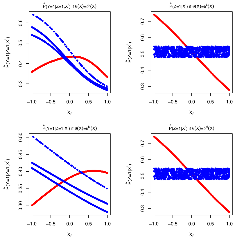
From the left panels of Figure S1, one can see that under correct model specification, is a non-monotone function of . Under mis-specifications of nuisance models, has three clusters, as for each value of , it is possible that or . The fitted values still depends on through the fitted values of . From the right panels of Figure S1, one can see that under correct model specification, is an expit function of . Under mis-specification of the instrumental density model, the fitted values do not depend on as is independent of .
S5.2 Implementation details in the simulation studies
We now describe the implementation details of the various estimators considered in the simulation studies:
- reg.ogburn
- dru.ogburn
- drw.ogburn
If , then we assume
If , then we assume
where
The higher order terms are added so that these models better approximate the truth.
In reg.ogburn, we obtain as the solution to the following estimating equations:
In dru.ogburn, first, we fit the model using R package glm. Then, we obtain as the solution to the estimating equation
In drw.ogburn, first, we fit the model using R package glm. Next, we estimate the optimal weighting function . If ,
if ,
where the model is fitted using the doubly robust estimator of Richardson et al., 2017 and obtained using R package brm, the model is fitted using the least squares method with the restriction that , and the model is fitted R package glm. Then, we obtain as the solution to the estimating equation
- mle.wang
- dru.wang
If , then we assume
In mle.wang, first, we fit the models and using the maximum likelihood estimation implemented in R package brm. Then, we fit the models and using the maximum likelihood estimation method based on the likelihood function of conditional on , and . The maximum likelihood estimator of is denoted as .
In dru.wang, first, we fit the model using R package glm. Next, we get and from , , and based on Proposition 2 of Wang and Tchetgen Tchetgen, 2018. Then, we obtain as the solution to the estimating equation
- dru.simple
If , then we assume
If , then we assume
In dru.simple, first, we fit the models , , and using R package glm. Then, we obtain as the solution to the estimating equation
where
- ls.abadie
If , then we assume
If , then we assume
In ls.abadie, first, we fit the model using R package glm. Then, we obtain the weighted least squares estimator by minimizing the following objective function
where
- mle.crude
If , then we assume
If , then we assume
In addition, for both cases, we assume
The above models are fitted using the maximum likelihood estimation method based on the likelihood function of conditional on and , and obtained using R package brm.
S5.3 Detailed simulation results
S5.4 The causal model assumed in the application to 401(k) data
S5.5 Implementation details in the application to 401(k) data
In the 401(k) data, since only eligible individuals may choose to participate in 401(k) plans, some model assumptions are different from those in the simulation studies. The model fitting methods are the same as that in Section S5.2. In the application, we focus on the case where . Models are fitted in a similar fashion as in Section S5.2.
- mle
- drw
Assume
- dru.ogburn
- drw.ogburn
Assume
- dru.simple
Assume
- ls.abadie
Assume
- mle.crude
Assume
| Bias (SE ) | ||||
|---|---|---|---|---|
| mle.bth | 0.28(0.35) | -3.5(0.78) | -0.092(0.71) | -3.0(1.2) |
| mle.bad | -20(0.42) | -15(0.80) | -48(1.2) | -18(2.1) |
| drw.bth | 0.55(0.36) | -4.1(0.82) | 0.54(0.77) | -5.6(1.5) |
| drw.psc | 0.060(0.38) | -5.9(1.0) | -0.38(1.2) | -12(2.7) |
| drw.opc | 0.55(0.36) | -3.9(0.79) | 0.49(0.75) | -5.3(1.4) |
| drw.bad | -10(0.40) | -9.6(1.1) | -28(1.4) | 25(3.3) |
| dru.bth | 1.3(0.44) | -5.8(1.0) | 1.8(0.84) | -8.1(1.7) |
| dru.psc | 1.2(0.44) | -6.1(1.0) | 1.9(0.84) | -9.0(1.7) |
| dru.opc | 0.94(0.39) | -4.5(0.86) | 0.99(0.78) | -6.5(1.5) |
| dru.bad | -14(0.48) | -27(1.4) | -28(0.98) | -12(2.4) |
| reg.ogburn.bth | -5.7(1.6) | -2.9(3.1) | 7.8(2.0) | -1.1(2.2) |
| reg.ogburn.bad | -9.0(0.25) | 100(0.23) | 140(5.6) | 93(3.6) |
| drw.ogburn.bth | 0.10(0.46) | -4.2(0.99) | 3.2(1.4) | -13(2.5) |
| drw.ogburn.psc | 1.3(0.46) | -8.2(1.3) | 7.7(1.9) | -18(3.5) |
| drw.ogburn.opc | -5.5(1.1) | -8.0(1.5) | 12(2.3) | 21(4.7) |
| drw.ogburn.bad | -120(3.1) | -170(6.0) | -40(2.6) | -9.4(5.8) |
| dru.ogburn.bth | 1.3(0.45) | -5.8(1.1) | 1.9(0.85) | -8.2(1.7) |
| dru.ogburn.psc | 1.5(0.49) | -9.1(1.3) | 3.1(0.90) | -11(2.0) |
| dru.ogburn.opc | -2.9(0.58) | -2.5(1.1) | 4.6(1.5) | 11(3.0) |
| dru.ogburn.bad | -130(3.2) | -190(6.4) | -47(1.0) | -41(3.7) |
| mle.wang.bth | 0.28(0.35) | -3.8(0.79) | ||
| mle.wang.bad | -27(0.40) | -1.5(1.1) | ||
| dru.wang.bth | 1.3(0.45) | -5.8(1.0) | ||
| dru.wang.psc | 1.2(0.45) | -6.3(1.0) | ||
| dru.wang.opc | 0.29(0.41) | -7.8(1.0) | ||
| dru.wang.bad | -20(0.52) | -24(1.5) | ||
| dru.simple.bth | 1.3(0.45) | -5.8(1.0) | 1.8(0.84) | -8.0(1.7) |
| dru.simple.psc | 1.2(0.44) | -6.2(1.0) | 1.9(0.84) | -8.8(1.7) |
| dru.simple.opc | 4.5(0.49) | -17(1.2) | -0.15(0.68) | 11(1.2) |
| dru.simple.bad | -16(0.48) | -17(1.3) | -34(0.70) | 18(1.5) |
| ls.abadie.bth | -0.19(0.37) | -4.1(0.93) | 0.42(0.79) | -11(1.6) |
| ls.abadie.bad | -23(0.88) | 22(1.2) | -32(1.9) | 7.7(3.6) |
| mle.crude | -2.8(0.10) | 60(0.19) | 0.36(0.25) | 51(0.42) |
| Bias/SD | ||||
| mle.bth | 0.02 | -0.14 | -0.00 | -0.08 |
| mle.bad | -1.53 | -0.61 | -1.25 | -0.28 |
| drw.bth | 0.05 | -0.16 | 0.02 | -0.12 |
| drw.psc | 0.01 | -0.19 | -0.01 | -0.14 |
| drw.opc | 0.05 | -0.15 | 0.02 | -0.12 |
| drw.bad | -0.79 | -0.28 | -0.66 | 0.24 |
| dru.bth | 0.09 | -0.18 | 0.07 | -0.15 |
| dru.psc | 0.08 | -0.19 | 0.07 | -0.16 |
| dru.opc | 0.08 | -0.17 | 0.04 | -0.13 |
| dru.bad | -0.94 | -0.61 | -0.89 | -0.15 |
| reg.ogburn.bth | -0.11 | -0.03 | 0.13 | -0.02 |
| reg.ogburn.bad | -1.16 | 14.18 | 0.81 | 0.82 |
| drw.ogburn.bth | 0.01 | -0.13 | 0.07 | -0.16 |
| drw.ogburn.psc | 0.09 | -0.20 | 0.13 | -0.16 |
| drw.ogburn.opc | -0.15 | -0.17 | 0.17 | 0.14 |
| drw.ogburn.bad | -1.48 | -1.07 | -0.49 | -0.05 |
| dru.ogburn.bth | 0.09 | -0.17 | 0.07 | -0.15 |
| dru.ogburn.psc | 0.10 | -0.22 | 0.11 | -0.17 |
| dru.ogburn.opc | -0.16 | -0.07 | 0.10 | 0.12 |
| dru.ogburn.bad | -1.53 | -1.10 | -1.47 | -0.35 |
| mle.wang.bth | 0.03 | -0.15 | ||
| mle.wang.bad | -2.16 | -0.04 | ||
| dru.wang.bth | 0.09 | -0.18 | ||
| dru.wang.psc | 0.09 | -0.19 | ||
| dru.wang.opc | 0.02 | -0.25 | ||
| dru.wang.bad | -1.24 | -0.52 | ||
| dru.simple.bth | 0.09 | -0.18 | 0.07 | -0.15 |
| dru.simple.psc | 0.09 | -0.19 | 0.07 | -0.16 |
| dru.simple.opc | 0.29 | -0.44 | -0.01 | 0.28 |
| dru.simple.bad | -1.07 | -0.41 | -1.54 | 0.36 |
| ls.abadie.bth | -0.02 | -0.14 | 0.02 | -0.22 |
| ls.abadie.bad | -0.84 | 0.57 | -0.54 | 0.07 |
| mle.crude | -0.83 | 10.02 | 0.04 | 3.76 |
| Coverage probability | ||||
|---|---|---|---|---|
| mle.bth | 95.6(0.502) | 95.8(1.25) | 95.4(1.12) | 96.4(2.02) |
| mle.bad | 65.4(0.662) | 91.0(1.38) | 46.3(2.00) | 94.6(3.38) |
| drw.bth | 94.7(0.513) | 95.2(1.31) | 96.9(1.21) | 95.9(2.34) |
| drw.psc | 95.4(0.561) | 95.5(1.65) | 97.6(2.43) | 97.4(4.20) |
| drw.opc | 95.0(0.505) | 95.6(1.25) | 96.1(1.19) | 96.1(2.30) |
| drw.bad | 87.0(0.614) | 95.3(1.82) | 91.8(2.94) | 96.8(5.54) |
| dru.bth | 94.5(0.636) | 94.6(1.59) | 96.3(1.46) | 96.9(2.61) |
| dru.psc | 94.8(0.639) | 95.0(1.62) | 96.3(1.46) | 97.6(2.65) |
| dru.opc | 93.8(0.564) | 94.8(1.34) | 96.1(1.31) | 96.9(2.33) |
| dru.bad | 79.6(0.732) | 91.3(2.35) | 87.4(1.61) | 98.2(3.28) |
| reg.ogburn.bth | 98.0(1.37) | 99.9(3.40) | 99.6(2.38) | 100.0(3.09) |
| reg.ogburn.bad | 75.6(0.318) | 0.1(0.284) | 99.9(4.81) | 86.1(3.78) |
| drw.ogburn.bth | 97.0(0.564) | 98.1(1.42) | 98.5(1.85) | 98.4(3.29) |
| drw.ogburn.psc | 95.4(0.689) | 95.7(2.01) | 99.7(2.95) | 99.9(5.18) |
| drw.ogburn.opc | 98.8(0.830) | 99.0(1.98) | 99.8(2.39) | 99.9(5.14) |
| drw.ogburn.bad | 2.2(2.84) | 72.5(5.62) | 99.7(3.06) | 99.9(6.55) |
| dru.ogburn.bth | 94.5(0.644) | 95.0(1.63) | 96.2(1.37) | 97.2(2.59) |
| dru.ogburn.psc | 93.4(0.692) | 94.3(2.03) | 96.9(1.51) | 97.3(2.85) |
| dru.ogburn.opc | 99.3(0.836) | 97.9(1.75) | 99.6(1.76) | 99.6(3.79) |
| dru.ogburn.bad | 1.6(2.95) | 64.0(5.81) | 91.6(1.39) | 99.6(4.27) |
| mle.wang.bth | 94.3(0.466) | 95.1(1.13) | ||
| mle.wang.bad | 41.1(0.564) | 94.3(1.41) | ||
| dru.wang.bth | 94.4(0.637) | 94.7(1.60) | ||
| dru.wang.psc | 94.8(0.643) | 94.7(1.65) | ||
| dru.wang.opc | 94.1(0.581) | 94.5(1.60) | ||
| dru.wang.bad | 68.0(0.786) | 92.1(2.47) | ||
| dru.simple.bth | 94.3(0.636) | 94.8(1.59) | 96.1(1.36) | 96.5(2.51) |
| dru.simple.psc | 94.6(0.641) | 94.5(1.63) | 96.1(1.38) | 96.8(2.57) |
| dru.simple.opc | 93.6(0.692) | 92.5(1.84) | 96.2(1.05) | 94.9(1.79) |
| dru.simple.bad | 76.4(0.706) | 94.2(2.16) | 69.3(1.05) | 93.8(2.27) |
| ls.abadie.bth | 94.8(0.593) | 95.5(1.57) | 96.4(1.24) | 95.6(2.56) |
| ls.abadie.bad | 87.3(0.898) | 94.5(1.50) | 93.1(2.03) | 95.7(3.86) |
| mle.crude | 84.3(0.127) | 0.0(0.228) | 94.0(0.303) | 6.3(0.524) |