Real Space Orthogonal Projector-Augmented-Wave Method
Abstract
The projector augmented wave (PAW) method of Blöchl makes smooth but non-orthogonal orbitals. Here we show how to make PAW orthogonal, using a cheap transformation of the wave-functions. We show that the resulting Orthogonal PAW (OPAW), applied for DFT, reproduces (for a large variety of solids) band gaps from the ABINIT package. OPAW combines the underlying orthogonality of norm-conserving pseudopotentials with the large grid spacings and small energy cutoffs in PAW. The OPAW framework can also be combined with other electronic structure theory methods.
I Introduction
A plane wave basis set is natural when studying periodic systems with DFT and post-DFT methods. Convergence with basis set is simply verified by increasing a single parameter, the kinetic energy cutoff. However, due to the fast oscillation of atomic core states, a direct all-electron treatment is prohibitive. One way to circumvent this problem is to replace the effect of the chemically inert core states by an effective pseudo-potential, and the resulting pseudo valence states are non-oscillatory.Reis et al. 2003; Willand et al. 2013 DFT using pseudo-potentials and a plane wave basis set has therefore become one of the most popular choices in computational chemistry and materials science. However, despite the formal simplicity of norm-conserving pseudo-potentials (NCPP), treatment of first-row elements and transition metals is still computationally demanding, due to the localized nature of and orbitals.Kresse and Hafner 1994; Hamann et al. 1979; Hamann 2013
The projector-augmented wave (PAW) method proposed by BlöchlBlöchl 1994; Kresse and Joubert 1999; Blöchl et al. 2003; Holzwarth et al. 1997 seeks to make softer pseudo wavefunctions by relaxing the norm-conserving condition. There are several different implementations of the PAW method (e.g., Tackett et al. 2001; Torrent et al. 2008; Enkovaara et al. 2010; Mortensen et al. 2005) with many successful applications.
In addition to the reduced kinetic energy cutoff, an advantage of the PAW method is that it provides means for recovering the all-electron orbitals, and these orbitals possess the right nodal structures in the core region. Therefore, PAW enables the calculation of quantities such as hyperfine parameters, core-level spectra, electric-field gradients, and the NMR chemical shifts, which rely on a correct description of all-electron wavefunctions in the core region.Pickard and Mauri 2001
The PAW method is based on a map between the smoothed pseudo wavefunctions and the all electron wavefunctions . Unlike NCPP where the wavefunctions retain their orthogonality, the pseudo wavefunctions in PAW satisfy a generalized orthogonality condition:
| (1) |
which leads to a generalized eigenproblem: where we introduced the 1-body Hamiltonian and overlap operator (both detailed later).
The fact that the pseudo-orbitals are not orthogonal complicates, however, the use of PAW for applications that rely on the orthogonality of molecular orbitals. These include some post-DFT methods, as well as several lower-scaling DFT methods, including the modified deterministic Chebyshev approach (see, e.g., Zhou et al. 2014) or stochastic DFT methods,Baer et al. 2013; Neuhauser et al. 2014a which are able to handle a large number of electrons (potentially hundreds of thousands for the stochastic approach) by filtering a function of an orthogonal Hamiltonian.
Here we solve the non-orthogonality problem by an efficient numerical transformation of the PAW problem to an orthogonal one,
| (2) |
with forming an orthogonal set, with the same norm as the all-electron orbitals (to be proved later). The key is that we show how to numerically apply the (or operator efficiently, without significantly raising the cost of applying the Hamiltonian.
The resulting approach retains one of the desirable features of NCPP, orthogonality of molecular orbitals, and we therefore label it Orthogonal PAW (OPAW). In addition to orthogonality, OPAW is also efficient because it is implemented in real space, exploiting the localization of atomic projector functions and partial waves.Enkovaara et al. 2010; Mortensen et al. 2005
OPAW provides a general framework, and can be combined with different electronic structure methods. Here we apply the method with the Chebyshev-filtered subspace iteration (CheFS) DFT approach, concentrating on the fundamental band gap of solids. We show below excellent agreement with PAW calculations from the ABINIT package.Torrent et al. 2008; Gonze et al. 2020 We also demonstrate that for many systems, PAW and OPAW band gaps converge with energy cutoff faster than NCPP.
Section II presents the OPAW theory. Results are presented in Section III, and conclusions follow in Section IV. Technical details are deferred to appendices.
II Theory
II.1 Orthogonal projector augmented wave
The basic relation in PAW is a map yielding the true molecular eigenstates, , from the smoother pseudo-orbitals
| (3) |
where is the atom index and runs over all the partial wave channels (a combination of principal, angular momentum and magnetic quantum numbers) associated with each atom; and are a true atomic orbital and a smoothed version which matches outside a small sphere around the atom (labeled the augmentation region). The atomic projectors are localized in the augmentation region, and are built to span the space within each augmentation sphere, i.e., in the sphere.
With some derivations, one arrives at the working equation of PAW, the generalized eigenproblem where
| (4) |
with and
| (5) |
The expressions for the Kohn-Sham effective potential and for are found in various references.Blöchl 1994; Torrent et al. 2008 While are only atom-dependent, and both depend on the on-site PAW atomic density matrices: , as well as the smooth density and the sum extends over the occupied states. The on-site atomic density matrices and the smooth density are the key components in PAW and together with the atomic information govern the updated quantities in each SCF cycle.
In many applications, however, it is desirable to work with an orthonormal collection of wavefunctions. As mentioned in the introduction, this can be achieved by the transformation:
| (6) |
resulting in
| (7) |
where .
As an example, in Fig. 2 we show 3D isosurfaces of , and for the orbital from a calculation of a single oxygen atom, as well as the associated 1D radial part obtained by projecting the 3D orbital to 1D. The three orbitals differ only in the core region; clearly has more structure in the core, while the oscillatory features are attenuated or absent in and . Furthermore, the magnitude of and are smaller than that of .
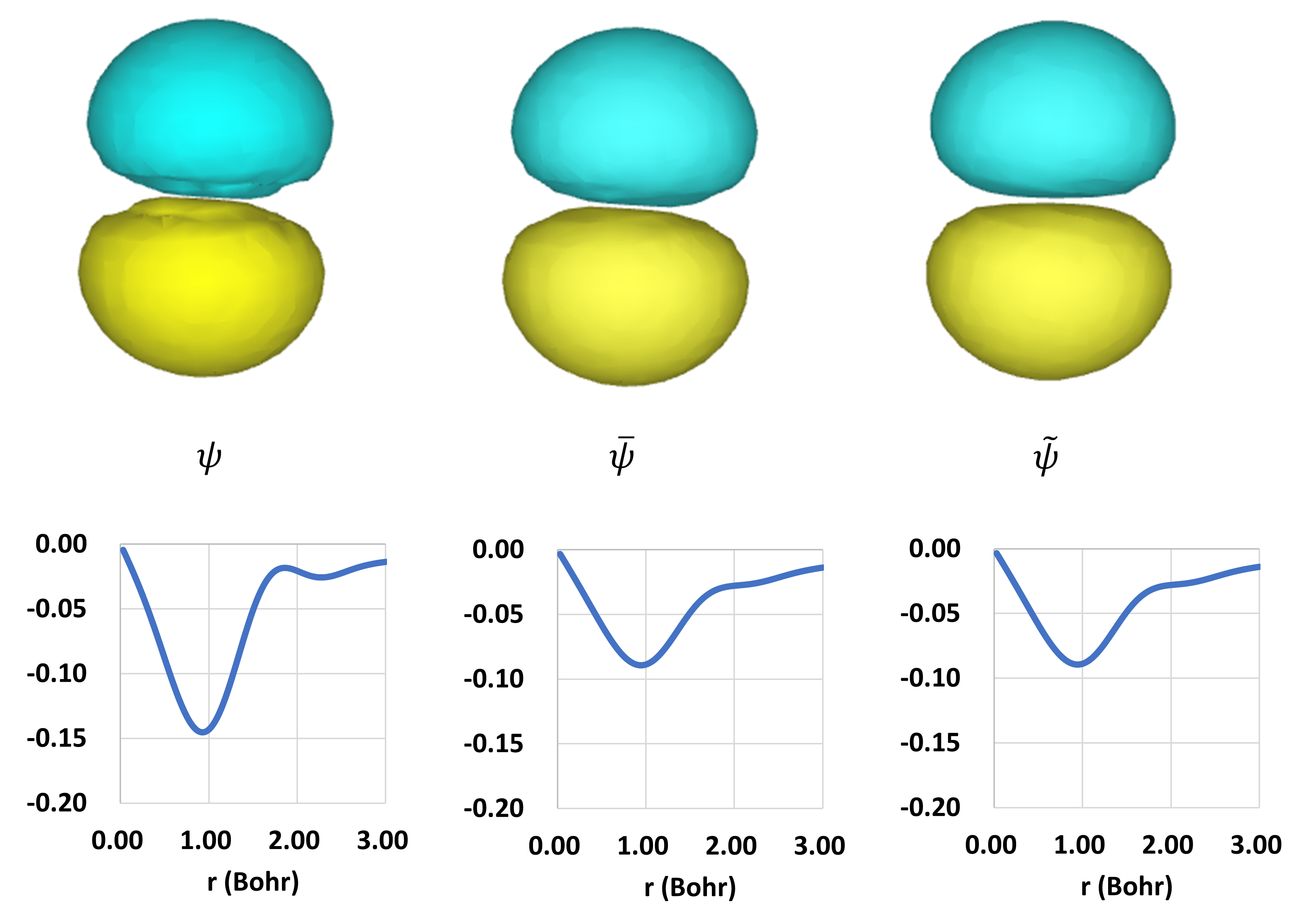
Obtaining
An efficient implementation of OPAW thus requires fast application of . For simplicity, we first consider the case where the augmentation spheres from different atoms do not overlap, so: if Therefore, we can separately rotate the } projectors around each atoms, so that is transformed into:
| (8) |
where the rotated projectors } are orthogonal and satisfy (see Appendix A). With this transformation, any power of is easily expressed; e.g.,
| (9) |
Since each is a projection operator (and all such operators are orthogonal) the proof of Eq. (9) becomes a trivial QM exercise emanating from the simple equation when is a projection opeator.
Next, note that the transformation operator between the orthogonal smooth molecular orbitals and the true ones is unitary
| (10) |
so . Due to the unitarity, the norm of the true molecular orbitals and the orthogonal smooth ones is identical, as mentioned.
Overall, we note that except for the automatic orthogonality, the algorithm is identical to the usual PAW. I.e., in an SCF cycle, with a given one-body Hamiltonian the orthogonal molecular orbitals (the solutions of Eq. (7)) are first found; then, we transform to the non-orthogonal orbitals, using Eq. (9), and use the usual prescription of the PAW algorithm to update in the PAW Hamiltonian.
Finally, note that the assumption of non-overlapping augmentation spheres is quite accurate, as shown in a latter section by the agreement between our results and ABINIT. Nevertheless, it is not exact; we could go beyond it by viewing our expression for as a pre-conditioner, as shown in Appendix B, and this would be pursured in further publications.
Avoiding singularities
The one caveat in Eq. (9) is the formal singularity when any of the is close to or below . Fundamentally, a value of indicates that the operator projects out the subspace spanned by .
For a start, note that negative values of between -1 and 0 do not pose mathematical difficulties in our formulation, but could indicate problems in the construction of the PAW parameters and in the eventual implementation, depending on the PAW code used (although they work fine in the ABINIT code used by us); see Ref. Holzwarth 2019 for details.
In practice, for most atoms we tested, were well above . We did encounter one case where is very close to – the GGA PAW parametrization of silicon taken from the website of the ABINIT PAW code,Jollet et al. 201411 1 https://www.abinit.org/ATOMICDATA/014-si/Si.LDA_PW-JTH.xml where . Fortunately the problem is trivially circumvented by replacing by where is a small positive number. The results are insensitive to . For example, for we tested (see Table 1) three different choices, and . The two lower values of gave results that agree completely with those using the LDA PAW file taken from the ABINIT website,Jollet et al. 201422 2 https://www.abinit.org/ATOMICDATA/014-si/Si.GGA_PBE-JTH.xml where was higher than . Even the large shift parameter, , led to only a slight deviation.
We also note that numerical problems could also arise from the compensation charge being negative. A solution to this problem is discussed in the literature.Holzwarth et al. 2001; Holzwarth 2019
| Grid spacing (Bohr) | 0.34 | 0.37 | 0.40 | 0.46 | |
| Gap (eV), LDA PAW | 5.97 | 5.97 | 5.94 | 5.85 | |
| Gap (eV), GGA PAW | 5.97 | 5.97 | 5.94 | 5.85 | |
| 5.97 | 5.97 | 5.94 | 5.85 | ||
| 5.95 | 5.95 | 5.92 | 5.83 |
II.2 Application of OPAW in DFT and technical details
The OPAW algorithm is general, and can be applied with any technique requiring an orthogonal Hamiltonian. Before talking about implementation of OPAW in DFT, note that a real space implementation of OPAW will require the inner product between atomic projectors and wavefunctions: . Such inner products are involved in determining the density matrices , as well as applying the operators and . In a real space formalism, the smooth wavefunctions are defined on a 3D grid. For computational efficiency, as long as the accuracy of the results is not affected the grid spacing for should be made as large as possible. On the other hand, the projector functions are short-ranged and in general show larger variation than the wavefunctions, so that evaluating the inner product directly on a coarse 3D grid would lead to large numerical errors.
To solve this problem, we adopted the method of Ono and Hirose,Ono and Hirose 1999 which connects the grid of the system with a set of finer grid points around each atom. Technical details regarding the Ono-Hirose method are given in Appendix C.
With a real-space implementation of OPAW in hand, we applied it along with the Chebyshev-filtered subspace iteration (CheFS) technique,Zhou et al. 2014 resulting in an efficient DFT program (OPAW-DFT). The idea of CheFS is described in Appendix D, along with a summary of the algorighm in Appendix E.
Furthermore, since we are working with periodic systems, we did k-point sampling. A brief account of using k-point sampling with OPAW is supplied in Appendix F.
III Results and discussion
III.1 Computational details
We did a set of calculations for periodic solids and report the calculated fundamental band gap. The geometries are taken from the ICSD database.33 3 https://icsd.fiz-karlsruhe.de/ A k-point mesh was used for each system.
We used the PBE GGA functional in all calculations.
For all calculations, the cutoff energy for the plane wave basis set, is related to the density cutoff-energy by , as is typical in plane-wave calculations. Note that the latter is related to the grid spacing for the density by . Thus, as usual, the grid used for the density is twice as dense (in each direction) then the spatial-grid for the plane waves.
As mentioned, to assist the SCF convergence we applied a DIIS procedurePulay 1980; Pulay 1982 when updating . At times, we have also applied a DIIS procedure for the Hamiltonian terms to assist SCF convergence.
For PAW calculations, we used the recommended atomic datasets from the ABINIT website.Jollet et al. 2014 There are two exceptions: the Sc atom, where the terms were large, more than 40 Hartree, and the Sr atom, where the terms exceed 1000 Hartree. In both cases this is due to a mismatch of the shape of the smooth and true atomic orbitals in the second, outer, d-shell. To simplify, we therefore generated new PAW potentials for Sc and Sr from the AtomPAW package,Holzwarth et al. 2001 using only one d-shell. For NCPP calculations, we used the recommended pseudo-potentials from the ABINIT website44 4 https://www.abinit.org/psps_abinit. More information on the PAW and NCPP datasets can be found in Supplementary Materials55 5 See Supplementary Material at [URL of Supplementary Material].
III.2 Results
Overall, DFT calculations produce two types of information. The first is forces and total energy, important for binding and molecular dynamics. Here, we concentrate on the second type of output from DFT: orbital energies and states, and here specifically the DFT HOMO-LUMO gap. The DFT gap often serves as preliminary approximation to the actual fundamental band gap,Zhan et al. 2003 and the Kohn-Sham orbitals and their energies are the basic ingredients for most beyond-DFT methods. Future papers will also examine the total energy and forces with OPAW, as well as the shape of the band structure.
We first examine the band-gap convergence with energy cutoff for an NaCl solid. We compared OPAW-DFT with ABINIT simulations using PAW or NCPP. The results are shown in Figure 2. For NaCl, our OPAW-DFT successfully reproduced the ABINIT results. Furthermore, the two PAW-based methods show better convergence with grid spacing than the NCPP-based method.

Secondly, we report the calculated fundamental band gap of a series of solids. A comparison of the converged results from ABINIT-PAW and OPAW-DFT is shown in Table 2. We also present the reference value from the work of Borlido et al.Borlido et al. 2019 The results indicate that OPAW-DFT reproduces ABINIT-PAW for a wide variety of systems, using generally the energy cutoff in ABINIT (with the advantage that in real-space we use the localization of the projector functions, so the cost of appying the Hamiltonian on a single function scales linearly with the size of the system.)
The table shows that for most solids both OPAW and ABINIT-PAW outperform NCPP, sometimes dramatically; e.g., for SiO2, the energy cutoff required for converging the band gap is 15 Hartree for the two PAW based methods, and 29 Hartree for ABINIT-NCPP calculation; for InP te difference is even more dramatic.
| OPAW-DFT | ABINIT-PAW | ABINIT-NCPP | Refe-renceBorlido et al. 2019 | ||||
|---|---|---|---|---|---|---|---|
| System | Gap | Gap | Gap | Gap | |||
| NaCl | 5.09 | 11 | 5.10 | 11 | 5.07 | 25 | 5.10 |
| CaO | 3.65 | 13 | 3.64 | 13 | 3.66 | 19 | 3.63 |
| PbS | 0.31 | 9 | 0.29 | 9 | 0.34 | 16 | 0.30 |
| InP | 0.68 | 10 | 0.65 | 10 | 0.69 | 23 | 0.71 |
| Si | 0.63 | 7 | 0.63 | 7 | 0.61 | 7 | 0.62 |
| SiO2 | 5.99 | 15 | 5.97 | 15 | 6.00 | 29 | 6.02 |
| ScNiSb | 0.28 | 17 | 0.25 | 15 | 0.29 | 34 | 0.30 |
| NiScY | 0.31 | 14 | 0.28 | 14 | 0.31 | 20 | 0.30 |
| LiH | 2.97 | 10 | 2.97 | 12 | 2.99 | 19 | 3.00 |
| KBr | 4.33 | 8 | 4.33 | 7 | 4.34 | 18 | 4.36 |
| K3Sb | 0.75 | 8 | 0.74 | 5 | 0.75 | 6 | 0.77 |
| CaCl2 | 5.41 | 10 | 5.42 | 13 | 5.40 | 20 | 5.43 |
| BN | 4.46 | 18 | 4.45 | 24 | 4.53 | 34 | 4.45 |
| BaCl2 | 5.04 | 8 | 5.04 | 8 | 5.05 | 10 | 5.03 |
| Ar | 8.70 | 9 | 8.69 | 11 | 8.70 | 10 | 8.71 |
| AlP | 1.58 | 9 | 1.57 | 9 | 1.58 | 12 | 1.58 |
| SrO | 3.30 | 13 | 3.30 | 13 | 3.32 | 13 | 3.26 |
To visualize the improvement in cutoff energy required for converging the fundamental band gap of solids to less than eV, we use histograms in Figure 3. The figure shows that PAW gives excellent results with cutoff energies that can be as low as 7 Hartree, and are generally (in the examples we studied) below 20 Hartree.

Finally, we note that in some approaches, for example stochastic methods for DFT, TDDFT, GW and Bethe-Salpeter Baer et al. 2013; Neuhauser et al. 2014a; Gao et al. 2015; Neuhauser et al. 2014b; Vlcek et al. 2017; Zhang et al. 2020; Rabani et al. 2015, the numerical cost is related directly to the number of spatial grid points rather than the number of plane waves; in those cases a choice of (rather than ) is better. Analog of Table 2 and Figure 3 for this choice can be found in the Supplementary Material 66 6 See Supplementary Material at[URL of Supplementary Material]. On average the required when is much smaller than that required when using (as done above), i.e. setting allows a much sparser real space grid.
IV Conclusions
The results in the previous section show that our efficient OPAW reproduces traditional PAW. The OPAW algorithm is easy to implement and combines the best of both worlds: the lower cutoff energy typically enabled by PAW and the orthogonality of norm-conserving pseudopotential approaches.
With the efficient methodology for acting with the Hamiltonian and overlap/inverse overlap, i.e., the simple application (on any function ) of , , and , we can combine PAW with other electronic structure theory methods, including our linear scaling stochastic TDDFT and GW methods,Neuhauser et al. 2014b; Vlcek et al. 2017; Gao et al. 2015 opening the door to significant (in some cases an order of magnitude) improvements in overall grid size and the reduction of the spectral range, and potentially even larger improvements in the cost of beyond-DFT approaches.
Finally, we note that an example where some of the developments here were applied is our recent large scale stochastic long-range exchange method for TDDFT using PAW.Zhang et al. 2020
Acknowledgements
We are grateful to Roi Baer, Eran Rabani, Vojtech Vlcek and Xu Zhang for helpful conversations. This work was supported by the NSF CHE-1763176 grant. Computational resources were supplied through the XSEDE allocation TG-CHE170058.
Appendix A: Transformation through
We start by a proof of Eq. (1). Since the molecular orbitals are orthogonal, and since , it follows that which given the definiton yields Eq. (1).
In the remainder we discuss the technical details of the transformation.
Given the initial operator:
| (A.1) |
the first step is to orthonormalize the projectors. For each atom, define a projector overlap matrix , and diagonalize it: , with unitary. Then, define a new set of projectors :
| (A.2) |
that will be orthogonal, Inverting Eq. (A.2) and substituting into Eq. (A.1) then gives:
| (A.3) |
where .
The next step involves diagonalization of the matrix , as , with unitary. It then readily follows that:
| (A.4) |
where are also orthogonal due to the unitarity of (Note that a diagonal representation of projectors is also done in NCPP, where diagonal projectors are used in representing the non-local potential.Hamann 2013)
Finally, when we apply the Ono-Hirose procedure, the bare are replaced by the processed ones, as in Eq. (C.3), i.e.,
| (A.5) |
These are not orthogonal on the rough-grid surrounding each molecule. We therefore repeat the orthogonalization procedure, Eqs. (A.1)-(A.4), with the overlap matrix now being replaced by , leading eventually to
| (A.6) |
where are orthogonal on the rough grid, .
Appendix B: Going beyond the non-overlapping augmentation spheres assumption
In this appendix we show how one could go beyond the non-overlapping augmentation sphere assumption. Let’s consider for simplicity exprssions using rather than . Then, the generic relation (the inversion of which is the crucial step in a Chebyshev propagation that iterates ) can be rewritten as
| (B.1) |
where and
| (B.2) |
while is a non-ovelapping () expression for as in Section II.A
| (B.3) |
and we use the abbreviated notation from there (but without assuming that different are orthorgonal). Note that this appendix is the only place in the paper where we give an explicit subscipt () to expressions obtained under the non-overlapping assumption.
Equation (B.1) could be solved by a Taylor expression in which measures the deviation from the non-overlapping spheres assumption. Recall that our results, obtained essetnially by assuming that , are all quite accurate. Therefore, even a single Taylor term should be extremely accurate, i.e.,
Appendix C: The Ono-Hirose transformation with a spline method and its implications in OPAW
The method of Ono and HiroseOno and Hirose 1999 is used to connect, for each atom, two sets of local grids. (The grids are specific to each atom, but for brevity we omit the atomic label in the following derivations.) One is a ’rough grid’ , consisting of a small cubic region of the 3D wavefunction grid, which encloses the augmentation sphere for the specific atom. The second is a ’fine grid’ , spanning the same volume but with more grid points and smaller grid spacing.
The overlap of the waveunctions and projectors should formally be performed on the fine grid. This requires, formally, interpolating the wavefunction from the rough grid (i.e., ) to the fine grid, as
| (C.1) |
where is a linear projection matrix. Earlier applications of the Ono-Hirose approach usually used cubic fitting,Ono and Hirose 1999; Enkovaara et al. 2010; Mortensen et al. 2005 but here we used a spline fit.
The key observation of the Ono-Hinose approach is then that the fine-grid overlap of the atomic projectors and the wavefunctions,
can be written as a rough-grid overlap
| (C.2) |
where and are the fine-grid and rough-grid volume elements, and
| (C.3) |
The key practical aspect in the Ono-Hirose transformation is the smoothing matrix, , connecting the fine and rough grids (Eq. (C.1)). Typically a cubic-fit approach is used; here we opted instead to use a spline fit matrix, which is separable.
| (C.4) |
where the matrices are obtained as explained below, and depend on the element only, not the specific atoms (the derivation is done for the case of equal grid spacings, , and is trivially extended in the general case).
For each different element a small padding region is added around the augmented region (typically of size 0.5 or 1Bohr, the results do not change if either value is used). Then the set of all points within a distance from the nucleus, where , is labeled as . Here, , and will be typically 6-14 for our grid parameters. The set will be denoted as the rough-1d grid in the direction.
We define then a fine 1D grid of size where is adjusted so that the fine grid spacing, is quite small, about Bohr (thus typically ). Further, we relabel as a matrix, with , .
The matrix is formally defined as the spline fit coefficient matrix, i.e., given a 1-d function on a rough grid, then the fine-grid spline interpolation is
| (C.5) |
While it is possible to derive formally, the simplest approach is to use a set of delta-functions. For example, to obtain use a spline fit subroutine with a input vector, feed it to a spline-fit interpolation program, and the resulting fine-grid vector will be exactly for .
Given the matrix (now again relabeled as ), the next stage is to rotate each fine-grid function to the rough grid, Eq. (C.3). This is easily done in stages due to the separability of Eq. (C.4), so that the total cost to transform each function is only about which works out to be about a one-time cost of 3,000-100,000 operations for each atom and for each projector, i.e., an overall negligibly small cost.
A side note: as it stands Eq. (C.4) and therefore the remainder of our derivation only applies to orthogonal cells; however, it is trivially generalized to other cyrstallographic cells, by replacing by non-orthogonal coordinates that are parrallel to the unit cell directions.
Finally, we note that there are alternatives to the Ono-Hirose technique, primarily the Mask Function Technique, where the radial functions are smoothed.Tafipolsky and Schmid 2006
Appendix D: Chebyshev-filtered subspace iteration
The OPAW algorithm is general, and can be applied with any technique requiring an orthogonal Hamiltonian. Here we combined our OPAW approach with the Chebyshev-filtered subspace iteration (CheFS) techniqueZhou et al. 2014 resulting in an efficient DFT program (OPAW-DFT).
In CheFS, with each iteration a more refined subspace is obtained, spanned by the lower energy orbitals. The Chebyshev filter
selectively enhances the occupied orbitals. Here is a Chebyshev polynomial of degree (typically taken as ) and its argument is a shifted Hamiltonian, where is set to be a little bit higher than LUMO energy and is set to be higher than the maximum eigenvalue of . The filter magnifies the weight of the lower end of the spectrum (energies below ). The number of states that the filter is operated on, labeled , needs to be somewhat larger than the number of occupied molecular orbitals.
Obtaining the action of on a function involves repeated applications of . In practice, we could either apply directly, or note that this is equivalent to . The latter is numerically slightly more efficient, since it involves only one application of an -type projector; practically, to obtain one simply need to replace the powers in Eq. (9) by . We verified that the two techniques give numerically the same results.
A summary of the structure of the OPAW-DFT algorithm is given next.
Appendix E: Summary of algorithm
For a given system, first,
- •
At this stage refers to each element in the system. From a given data set of atomic (typically contained in an “XML” file) construct the matrix, as well as several small-atom matrices needed for the PAW algorithm. Construct a new set of orthogonal orbitals, , that are a linear combination of , and extract the coefficients (Appendix A). Shift to be above -1 if necessary.
- •
Starting at this next stage, refers to each atom separately. Use the Ono-Hirose transformation (Appendix C) to form each on a small rough-grid around each atom. Similarly form and orthogonalize them (Appendix C) to form that are orthogonal on the grid. A new set of is then produced; again shift each to be above -1 if necessary.
Then start the SCF algorithm, presented first in terms of the orthogonal Hamiltonian, . All expressions now refer to the sparse 3D grid.
Pick a set of random plane-wave orbitals, (See Appendix F for details of the k-point sampling.) Orthogonalize them, and then do the following loop till convergence:
- •
Fourier transform the orbitals to the equivalent density-based spatial grid, . Form
- •
From , calculate the atomic density-type matrices, and construct the smooth density, DFT potential, and the terms. We adopted the routines of ABINIT for this stage.
- •
Starting at the 2nd iteration, we apply at this stage a DIIS iteration on the DFT potential, and potentially also on the terms.
- •
Apply the -th degree Chebyshev operator; symbolically assign . This could be done either totally at the spatial grid level, or alternately, one could at each stage (i.e., after each application of ) transfer back to the plane-wave grid, keeping only values of with energies below and then convert back to . There is no difference in the accuracy using either approach.
- •
At the end of the Chebyshev iteration, transfer to the plane-wave grid, orthogonalize the resulting functions , rotate back to space, diagonalize the matrix in the resulting basis of vectors, and rotate accordingly (with the resulting vectors again labeled .
- •
Based on the resulting orbital energies, assign occupation numbers. Repeat the cycle till SCF convergence (typically 10-20 times).
The algorithm is only slightly modified if we choose to replace the orthogonal by . In that case the only modifications are that we directly iterate , and at the end of each Chebyshev series we need to use general orthogonalization, so
Appendix F: k-point sampling
For periodic systems, the plane-wave wavefunctions are given by Bloch waves, where samples the first Brillouin zone, and are periodic. The modifications are therefore straightforward, exactly analogous to PAW and NCPP: Given a periodic Bloch state on a 3D unit cell grid, define a -dependent Hamiltonian as , with (in the spatial basis):
| (F.1) |
I.e., in each application the molecular orbital is multiplied once by , the projection performed for all atoms, and the resulting orbital is multiplied again by
Within the operator, the terms are similarly calculated, and the kinetic energy with the kinetic energy operator obtained as usual by passing to Fourier space (i.e., producing ), multiplying by , and transforming back.
References
- Reis et al. (2003) C. L. Reis, J. Pacheco, and J. L. Martins, Physical Review B 68, 155111 (2003).
- Willand et al. (2013) A. Willand, Y. O. Kvashnin, L. Genovese, Á. Vázquez-Mayagoitia, A. K. Deb, A. Sadeghi, T. Deutsch, and S. Goedecker, The Journal of chemical physics 138, 104109 (2013).
- Kresse and Hafner (1994) G. Kresse and J. Hafner, Journal of Physics: Condensed Matter 6, 8245 (1994).
- Hamann et al. (1979) D. Hamann, M. Schlüter, and C. Chiang, Physical Review Letters 43, 1494 (1979).
- Hamann (2013) D. Hamann, Physical Review B 88, 085117 (2013).
- Blöchl (1994) P. E. Blöchl, Physical review B 50, 17953 (1994).
- Kresse and Joubert (1999) G. Kresse and D. Joubert, Physical review b 59, 1758 (1999).
- Blöchl et al. (2003) P. E. Blöchl, C. J. Först, and J. Schimpl, Bulletin of Materials Science 26, 33 (2003).
- Holzwarth et al. (1997) N. Holzwarth, G. Matthews, R. Dunning, A. Tackett, and Y. Zeng, Physical Review B 55, 2005 (1997).
- Tackett et al. (2001) A. Tackett, N. Holzwarth, and G. Matthews, Computer Physics Communications 135, 348 (2001).
- Torrent et al. (2008) M. Torrent, F. Jollet, F. Bottin, G. Zerah, and X. Gonze, Computational Materials Science 42, 337 (2008).
- Enkovaara et al. (2010) J. Enkovaara, C. Rostgaard, J. J. Mortensen, J. Chen, M. Dułak, L. Ferrighi, J. Gavnholt, C. Glinsvad, V. Haikola, H. Hansen, et al., Journal of Physics: Condensed Matter 22, 253202 (2010).
- Mortensen et al. (2005) J. J. Mortensen, L. B. Hansen, and K. W. Jacobsen, Physical Review B 71, 035109 (2005).
- Pickard and Mauri (2001) C. J. Pickard and F. Mauri, Physical Review B 63, 245101 (2001).
- Zhou et al. (2014) Y. Zhou, J. R. Chelikowsky, and Y. Saad, Journal of Computational Physics 274, 770 (2014).
- Baer et al. (2013) R. Baer, D. Neuhauser, and E. Rabani, Physical review letters 111, 106402 (2013).
- Neuhauser et al. (2014a) D. Neuhauser, R. Baer, and E. Rabani, The Journal of chemical physics 141, 041102 (2014a).
- Gonze et al. (2020) X. Gonze, B. Amadon, G. Antonius, F. Arnardi, L. Baguet, J.-M. Beuken, J. Bieder, F. Bottin, J. Bouchet, E. Bousquet, N. Brouwer, F. Bruneval, G. Brunin, T. Cavignac, J.-B. Charraud, W. Chen, M. Côté, S. Cottenier, J. Denier, G. Geneste, P. Ghosez, M. Giantomassi, Y. Gillet, O. Gingras, D. R. Hamann, G. Hautier, X. He, N. Helbig, N. Holzwarth, Y. Jia, F. Jollet, W. Lafargue-Dit-Hauret, K. Lejaeghere, M. A. L. Marques, A. Martin, C. Martins, H. P. C. Miranda, F. Naccarato, K. Persson, G. Petretto, V. Planes, Y. Pouillon, S. Prokhorenko, F. Ricci, G.-M. Rignanese, A. H. Romero, M. M. Schmitt, M. Torrent, M. J. van Setten, B. V. Troeye, M. J. Verstraete, G. Zérah, and J. W. Zwanziger, Comput. Phys. Commun. 248, 107042 (2020).
- Holzwarth (2019) N. Holzwarth, Computer Physics Communications 243, 25 (2019).
- Jollet et al. (2014) F. Jollet, M. Torrent, and N. A. W. Holzwarth, Computer Physics Communications 185, 1246 (2014).
- (21) https://www.abinit.org/ATOMICDATA/014-si/Si.LDA_PW-JTH.xml.
- (22) https://www.abinit.org/ATOMICDATA/014-si/Si.GGA_PBE-JTH.xml.
- Holzwarth et al. (2001) N. Holzwarth, A. Tackett, and G. Matthews, Computer Physics Communications 135, 329 (2001).
- Ono and Hirose (1999) T. Ono and K. Hirose, Physical Review Letters 82, 5016 (1999).
- (25) https://icsd.fiz-karlsruhe.de/.
- Pulay (1980) P. Pulay, Chemical Physics Letters 73, 393 (1980).
- Pulay (1982) P. Pulay, Journal of Computational Chemistry 3, 556 (1982).
- (28) https://www.abinit.org/psps_abinit.
- (29) See Supplementary Material at [URL of Supplementary Material].
- Zhan et al. (2003) C.-G. Zhan, J. A. Nichols, and D. A. Dixon, The Journal of Physical Chemistry A 107, 4184 (2003).
- Borlido et al. (2019) P. Borlido, T. Aull, A. W. Huran, F. Tran, M. A. Marques, and S. Botti, Journal of chemical theory and computation 15, 5069 (2019).
- Gao et al. (2015) Y. Gao, D. Neuhauser, R. Baer, and E. Rabani, Journal of Chemical Physics 142, 034106 (2015).
- Neuhauser et al. (2014b) D. Neuhauser, Y. Gao, C. Arntsen, C. Karshenas, E. Rabani, and R. Baer, Physical Review Letters 113, 076402 (2014b).
- Vlcek et al. (2017) V. Vlcek, E. Rabani, D. Neuhauser, and R. Baer, Journal of Chemical Theory and Computation 13, 4997 (2017).
- Zhang et al. (2020) X. Zhang, G. Lu, R. Baer, E. Rabani, and D. Neuhauser, Journal of Chemical Theory and Computation 16, 1064 (2020).
- Rabani et al. (2015) E. Rabani, R. Baer, and D. Neuhauser, Physical Review B 91, 235302 (2015).
- (37) See Supplementary Material at[URL of Supplementary Material].
- Tafipolsky and Schmid (2006) M. Tafipolsky and R. Schmid, The Journal of chemical physics 124, 174102 (2006).